Article
Scaled Boundary Finite Element Method for
Two-Dimensional Linear Multi-Field Media
Chung Nguyen Van
1,a, Jaroon
Rungamornrat
1,b,*, and Phoonsak
Pheinsusom
2,c1 Applied Mechanics and Structures Research Unit, Department of Civil Engineering, Faculty of Engineering, Chulalongkorn University, Thailand
2Department of Civil Engineering, Faculty of Engineering, Chulalongkorn University, Thailand E-mail: a[email protected], b[email protected] (Corresponding author), c[email protected]
Abstract. This paper presents an efficient and accurate numerical technique, based on a scaled boundary
finite element method (SBFEM) that is capable of solving two-dimensional, second-order, linear, multi-field boundary value problems. Basic governing equations are established in a general, unified context allowing the treatment of various classes of linear problems such as state heat conduction problems, steady-state flow in porous media, linear elasticity, linear piezoelectricity, and linear piezomagnetic and piezoelectromagnetic problems. A scaled boundary finite element approximation is also formulated within a general framework integrating the influence of the distributed body source, general boundary conditions, contributions of the general side-face data, and the flexibility of scaled boundary approximations. Standard procedures for numerical integration, search of eigenvalues and eigenvectors, determination of particular solutions, and solving a system of linear algebraic equations are adopted. After fully tested with available benchmark solutions, the proposed SBFEM is applied to solve various classes of linear problems under different scenarios to demonstrate its vast capability, computational efficiency and robustness.
Keywords: Multi-field problems, SBFEM, surface flux, state variables, scaled boundary coordinates.
ENGINEERING JOURNAL Volume 21 Issue 7
1.
Introduction
A scaled boundary finite element method (SBFEM) has been found an attractive alternative analysis tool in the modelling of various problems in applied mechanics for the past two decades [1-12]. The method is recognized as a semi-analytical technique combining features of both analytical schemes and the finite element approximation and, due to the reduction of a spatial dimension in the discretization, it can be also categorized as a particular type of boundary element methods (BEMs). However, the key difference between the SBFEM and conventional BEMs is that the former is generally free of fundamental solutions; as a direct consequence, the non-trivial numerical treatment of singular integrals is not required. The concept of the SBFEM was originally introduced by Wolf and Song [13-15] using the mechanical-based approach to properly and efficiently model linear elastic unbounded media in the dynamic analysis of soil-structure interactions. To further reduce the complexity of the formulation presented in the original work, other techniques such as the standard weighted residual procedure and the principle of virtual work were also utilized to obtain the scaled boundary finite element equations [16-18]. As a result of the computational efficiency of the SBFEM in modelling unbounded media and the reduction of the discretization cost, various researches have been continuously and increasingly conducted, since its first emergence, to introduce other novel aspects and further enhance its capability.
In recent years, the SBFEM has been also applied to solve various boundary value problems. One salient feature of the SBFEM is that the whole domain can be generated by scaling its boundary with respect to a single point termed the scaling center. The SBFEM only requires meshing on a representative boundary of the domain and does not involve fundamental solutions. For a domain with the complex geometries, its interior can be discretized into sub-domains to satisfy the scaling requirement. For fracture problems, the scaling center is commonly located at the crack tip and, as a result, the stress field can be expressed analytically along the direction radiating from the crack tip. As a result, the strength of singularity and associated information can be directly and accurately calculated from the obtained solution [19, 20]. Based on this positive feature, the method has been extensively utilized in the investigation and simulations of fracture problems under various scenarios such as crack formation, static and dynamic crack propagation, and transient responses of bodies containing interfacial cracks, stress singularities and bi-material interfaces [21, 22]. In the modelling of wave propagations, the SBFEM has been also widely employed to study elastic guided waves in an unbounded domain and the radiation and diffraction of linear water waves in shallow water with sidewalls [23-25]. Results from those investigations demonstrated that the SBFEM generally yields more accurate numerical solutions and is more computationally efficient, in terms of the number of degrees of freedom involved, than other existing approaches. Li et al. [26] applied the SBFEM to investigate the structural behavior of offshore monopoles with the influence of the ocean wave loads. The basic concept of the SBFEM was adopted to formulate the governing monopole’s equation and the analytical wave equation. Later, Li et al. [6, 7] extended the SBFEM to study three-dimensional wave-pile problems with the emphasis on the wave behavior and pile-group responses. In their formulation, the scaled boundary finite element approximation is applied to Helmholtz equation by separating the vertical component from the velocity potential. The two-dimensional SBFEM was adopted to examine the wave field near the free surface level. Results from these studies indicated that the SBFEM is an accurate and efficient computational tool for the analysis of wave problems and wave-structure interactions. However, their formulation and implementations were still limited to particular settings.
circumferential direction. This particular technique was then applied to solve a number of standard linear elasticity problems and the technique was found to offer higher and better rate of convergence than the original SBFEM. Additionally, He et al. [32] investigated the possibility of using the Fourier shape functions in the SBFEM. The developed technique was then used to solve elastostatics and steady-state heat transfer problems. It was found that the accuracy and convergence of numerical solutions were better than those of results obtained from using the polynomial shape functions and an element-free Galerkin scheme.
Applications of the SBFEM to the analysis of linear problems involving piezoelectric materials have also been recognized in the literature. Liu and Lin [4] used the SBFEM to investigate two-dimensional electrostatic problems. Li et al. [5] developed the SBFEM to solve two-dimensional, linear piezoelectric fracture problems. The stress and electric displacement intensity factors for both static and dynamic cases were calculated directly from results of the SBFEM. It was indicated that the technique requires no asymptotic solution, no local mesh refinement, and no special treatment around the crack tip. Recently, Dieringer and Becker [33] employed the SBFEM to investigate linear problems within the framework of a classical laminated plate theory. In their study, the scaled boundary finite element equations for composites were formulated in terms of the displacement, and the stress singularity at a notch was fully examined. They also demonstrated that the enhanced SBFEM can evaluate the singular stress field as an explicit function of the notch opening displacement. Li et al. [34] and Li et al. [11] also employed the SBFEM to perform two-dimensional simulations of dynamic cracks and interfacial cracks in piezoelectric composites and also study the influence of thermal loads on the fracture response. While the SBFEM has been applied successfully to solve linear piezoelectric problems, the underlying formulation and existing implemented procedures are still limited to certain scenarios and, in particular, the extension of the technique to treat other general coupled-field media has not been found in the literature.
Other recent applications of the SBFEM have been also recognized. For instance, Ooi et al. [9,10] developed an efficient procedure based on the SBFEM together with polygon elements for simulating dynamic crack propagation in elastic media; He et al. [35] presented the SBFEM for the numerical analysis of two-dimensional elastic bodies with the rotationally periodic symmetry and subjected to arbitrary loading conditions; and, most recently, Vu and Deeks [8] integrated the information of the fundamental solutions into the scaled boundary finite element method and then used the technique to investigate problems in linear elasticity with concentrated loads. As become evident from the vast amount of related publications, researches on both the novel development and the enhancement of existing SBFEM have continuously and increasingly grown. However, most of existing SBFEMs were developed specifically for problems considered and this, as a consequence, limits its generality and flexibility to treat general field problems under various scenarios when compared with standard finite element methods. A systematic generalization of the SBFEMs to treat a broader class of boundary value problems obviously requires further rigorous investigations.
The present study aims to offer the SBFEM capable of solving two-dimensional, linear, second-order, multi-field boundary value problems. The key and novel feature is that all basic field equations governing responses of interest are formulated in a general framework allowing various types of linear problems such as steady-state heat conduction and flow in porous media, Laplace’s equation, linear elasticity, linear piezoelectricity and other coupled-field problems to be treated in a unified manner. In addition, the treatment of distributed body source, general boundary conditions, prescribed conditions on the side faces, and the scaled boundary approximations are integrated in the implementation.
2.
Problem Formulation
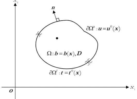
Consider a two-dimensional body occupying a region in 2
as shown schematically in Fig. 1. The region is assumed smooth in the sense that all involved mathematical operators (e.g., integrations and differentiations) can be performed on this region. In addition, the boundary of the body , denoted by , is assumed piecewise smooth and an outward unit normal vector at any smooth point on is denoted by n{ }n n1 2 T. More restrictions about the geometry of the body pertained in the present
study will be posed later as is appropriate. A two-dimensional Cartesian coordinate system { ; , }0 x x1 2 with
In particular, lower-case Greek subscripts range from 1 to 2 whereas upper-case subscripts range from 1 to {1, 2,3,...}
and repeated subscripts imply the summation over their range unless stated otherwise.
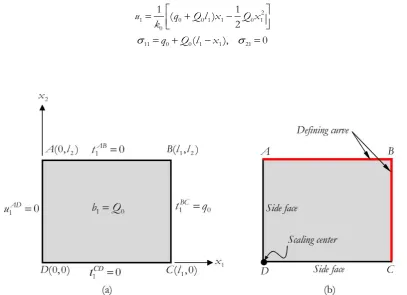
Fig. 1. Schematic of two-dimensional, multi-field body subjected to external excitations.
The body is made of a homogeneous material with its behavior completely characterized by 42 constants
denoted by a set {E IJ } and subjected to a prescribed distributed body-source field, denoted by a -component vector field ( ) { ( ) ( ) ... ( )}1 2
T
b b b
b x
x
x
x
. In the present study, the constants E IJ are assumed to satisfy the symmetry E IJ E JI . Responses of the body due to the distributed body-source( )
b x are assumed to be completely described by following three fields: the state variable ( )u x , the state-variable gradient ( ) x , and the body flux ( ) x . The state variable ( )u x contains components denoted by ( )uJ x and is represented, in a vector form, by
1 2
( ) { ( ) ( ) ... ( )}u u u T
u x
x
x
x
(1)The state-variable gradient ( ) x and the body flux ( ) x contain 2 components denoted by J and J
, respectively, and they can be also represented in a vector form by
11 12 1 21 22 2
( ) { ( ) ( ) ...
( ) ( ) ( ) ...
( )}T
x
x
x
x
x
x
x
(2)11 12 1 21 22 2
( ) { ( )
x
x
( ) ...x
( )x
( )x
( ) ...x
( )}x
T
(3)In addition, the surface flux at any smooth point x on the boundary is denoted by a -component vector
1 2
( ) { ( ) ( ) ... ( )}t t t T
t x
x
x
x
. The boundary of the given body can be decomposed into two disjoint portions; one is denoted by u where the state variable u is fully prescribed (u u x
0( )u
x where
u x
0( ) is a prescribed vector) and the other is denoted by t where the surface fluxt
is fully prescribed (i.e.,
t t x
0( ) x t wheret x
0( ) is a prescribed vector). In the present study, theprescribed vector-value functions ( )b x ,
u x
0( ) andt x
0( ) are assumed sufficiently smooth to ensure theexistence of the responses u u x ( ), ( )x and ( )x .
[image:4.595.165.431.125.317.2]piezomagnetic and piezoelectromagnetic solids, etc.) to be treated in a unified manner. The integer is used as a key parameter to indicate the type of problems. For instance, 1 corresponds to steady-state heat condition problems, problems of Darcy’s flow in porous media, and membrane problems, and
;
{ ( ); ( ); ( ); ( )u x x x b x E IJ ; }t represents {temperature; temperature gradient; heat flux; heat source; thermal conductivity; surface heat flux}, {fluid pressure; pressure gradient; fluid flux; source and sink; permeability; surface flux}, and {deflection; slopes; resultant shear force; distributed transverse load; membrane stiffness; end shear force}, respectively; 2 corresponds to linear elasticity problems and
;
{ ( ); ( ); ( ); ( )u x x x b x E IJ ; }t represents {displacement; displacement gradient; stress; body force; elastic constants; traction}; 3 corresponds to linear piezoelectric and piezomagnetic problems and
;
{ ( ); ( ); ( ); ( )u x x x b x E IJ ; }t represents {displacement and electric potential; gradients of displacement and electric potential; stress and electric induction; body force and body charge; elastic constants, piezoelectric constants, dielectric permittivities; traction and surface charge} and {displacement and magnetic potential; gradients of displacement and magnetic potential; stress and magnetic induction; body force and magnetic body source; elastic constants, piezomagnetic constants, magnetic permeabilities; traction and surface magnetic induction}, respectively; and 4 corresponds to linear piezoelectromagnetic problems and { ( ); ( ); ( ); ( )u x x x b x ;E IJ ; }t represents {displacement, electric and magnetic potentials; gradients of displacement, electric and magnetic potentials; stress, electric and magnetic inductions; body force, body charge, magnetic body source; elastic, piezoelectric, piezomagnetic and electromagnetic constants, dielectric permittivities, magnetic permeabilities; traction, surface charge, surface magnetic induction}.
The fundamental laws of conservation (e.g., conservation of linear and angular momentum, conservation of mass, conservation of heat flow, etc.), the linear constitutive laws (e.g., Darcy’s law, Fourier’s law, Hookes’ law, generalized Hookes’ law, etc), and the laws of kinematics (e.g., strain-displacement relations, electric-potential-field relations, etc.) are employed to form the basic governing field equations and they are expressed in a concise and unified form as follows:
T
L
b 0
(4)
D
(5)
Lu
(6)where a superscript “T” indicates a matrix transpose operator, D is a 2 2 -matrix termed the modulus
matrix, and L represents the linear differential operator defined, in terms of a 2 -matrix, by
1 2 1 2
1 2 1 2
; ,
x x x x
I
0
I
0
L
L
L
L
L
0
I
0
I
(7)with I and 0 denoting a -identity matrix and a -zero matrix, respectively. It should be remarked that entries of the modulus matrix D can be simply obtained from the set {E IJ } by properly considering the definition of the vectors and (i.e., E1JK1DJK , E1JK2 DJ K, , E2JK1DJ,K
and E2JK2 DJ ,K ) and, due to the symmetry of E IJ , the modulus matrix D is obviously symmetric.
By applying the law of conservation at any smooth point x on the boundary , the surface flux ( )t x
can be related to the body flux ( ) x and the outward unit normal vector ( ) { ( ) ( )}1 2
T
n n
x
x
x
n by
n1 n2
t
I
I
(8)Other useful relations such as that directly relating the body flux and the state variable and one connecting the surface flux and the state variable on the boundary can be readily obtained as
( )
D Lu
n1 n2
( )
t
I
I
D Lu
(10)2.1.
Weak Formulation
A standard weighted residual technique is adopted along with the integration by parts via divergence theorem to obtain a weak-form statement of the above problem. By first taking the inner product of (4) and any sufficiently smooth weight function ( ) { ( ) ( ) ... ( )}1 2
T
w w w
w x x x x , integrating the result over the body , and then applying an identity (wJJ), w LT T (Lw)T, it leads to
(Lw
)T
dA
(wJ J), dA
w b
T dA (11)By applying divergence theorem to the first integral on the right hand side (11) and then enforcing the boundary term (8), it gives rise to
( )T dA T dl T dA
Lw
w t
w b
(12)By further replacing the body flux
σ
appearing in (12) by that associated with the state variable via the relation (9), it finally yields( )T ( )dA T dl T dA
Lw D Lu
w t
w b
(13)It should be apparent from the above formulation that the weak-form Eq. (13) is valid for an arbitrary choice of the weight function w. Only restriction placed on the weight function is the smoothness requirement to ensure the integrability of all integrals appearing in (13). This can be achieved by requiring the weight function and their first partial derivatives square integrable, i.e.,
( ) (T ) T dA
Lw
Lw
w w
(14)2.2.
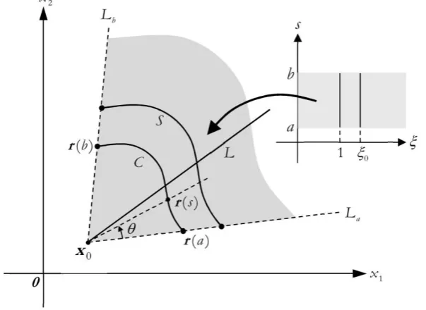
Scaled Boundary Coordinate TransformationLet x0(x10,x20) be a point in
2 and C be a simple, piecewise smooth curve in 2 parameterized by
a function 2
10 ˆ1 20 ˆ2
:s [ , ]a b (x x s x( ), x s( ))
r
as shown in Fig. 2. Let ( ) s be the circumferential angle of a point ( )r s on the curve C measured from a straight line connecting x and 0( )a
r to a straight line connecting x and ( )0 r s (see Figure 2). The simple curve C considered here can be
either closed (i.e., ( )r a r( )b ) or opened (i.e., ( )r a r( )b ) and, in addition, it must not contain the point
0
x and satisfies the conditions [0, 2 ] and d/ds 0 s ( , )a b . Now, let us introduce the following coordinate transformation
0 ˆ( )s
x x x (15)
where 0. It is evident from the coordinate transformation (15) that (i) any straight line 0,a s b
in the s plane is mapped to a curve S in the x1x2plane which is simply a scaled version of the curve C about x and (ii) any straight line 0 0,s s 0 [ , ]a b in the s plane is mapped to a semi-infinite
straight line L in the x1x2 plane starting from x and passing through the point 0 r( )s0 on the curve C
(also see Figure 2). In addition, a straight line 0,a s b in the s plane is mapped to a single point
0
curve C which is termed the defining curve. The coordinates and s are termed the scale boundary coordinates. Clearly, the transformation (15) maps the region 0,a s b in the s plane into a region in the
1 2
x x plane bounded by the two straight lines L and a L (i.e., a shaded region shown in Figure 2). From b
the coordinate transformation (15), a differential line dζ { }d ds T at any point ( , ) s in the s plane is
related to a differential line dx{dx dx1 2}T at any point
1 2
[image:7.595.141.443.179.399.2]( ,x x ) in the x1x2 plane by
Fig. 2. Schematic of a scaling centre
x
0 and a defining curve C .
1 1 1 2 1
2 2 2 1
ˆ ˆ / 1 ˆ / ˆ /
;
ˆ ˆ / ˆ / ˆ /
x dx ds dx ds dx ds
d d d d d d
x dx ds J x x
x T ζ
ζ T
x
x
(16)where J x dx ds x dx ds ˆ ˆ1 2/ ˆ ˆ2 1/ . By setting dζ (d)m where m is a unit vector and d is the length of dζ , it can be readily verified that the length of dx, denoted by dl, is given by
dl dx dx T T m m d
(17)For following two special cases: (i) m{1 0}T, dd and (ii) m{0 1}T, d
ds, the relation (17)reduces, respectively, to
2 2
1 2
ˆ ˆ
( ) , ( )
dl J s d
J s x x (18)
2
21 2
ˆ ˆ
( ) , ( ) / /
s s
dl J s ds J s
dx ds dx ds (19) Similarly, the differential area d ds
at any point ( , )
s in the
s plane can be related to the differential area dA at any point ( ,x x in the 1 2) x1x2 plane bydA J d ds
(20) From the chain rule for differentiations, the partial derivative of any function with respect to the coordinate
2 2 1 1 1 2 ˆ ˆ 1
ˆ ˆ 1
dx x
x ds
dx
J x
x ds s
(21)
The linear differential operator L given by (7) can be now expressed in terms of partial derivatives with respect to the coordinates
and s by1 2 1 s
L b b (22)
where b1 and b2 are 2 -matrices defined by
2 2 1 2 1 1 ˆ ˆ 1 1 , ˆ ˆ dx x ds dx x J J ds
I
I
b
b
I
I
(23)In the present study, we focus only on a body whose geometry can be completely described by a single scaling center. In particular, there must exist the scaling center x0 and defining curve C such that there
exists a region [ , ] [ , ] 1 2 s s1 2 in the
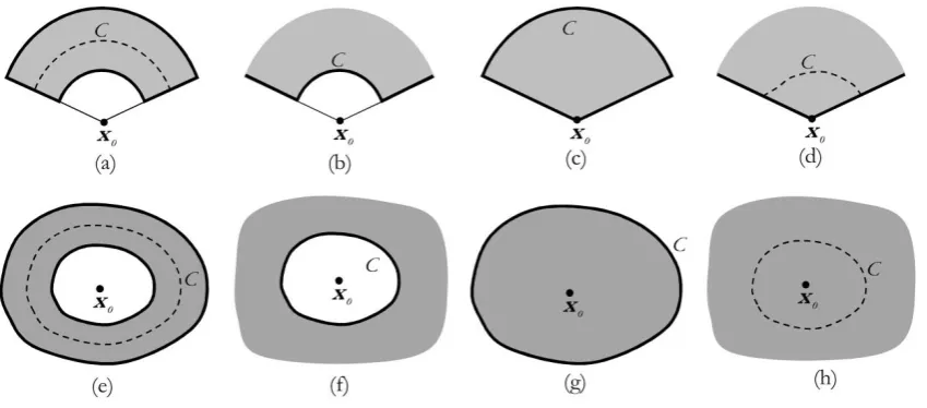
s plane that is mapped into the region in the x1x2 planevia the transformation (15). If the defining curve C is opened, the body is said to be opened and portions of the boundary associated with s s 1and s s 2 are termed the side faces (see Figure 3(a), (b), (c) and (d)).
If the defining curve is closed, the body is said to be closed and the boundary contains no side face (see Figure 3(e), (f), (g) and (h)). If 2 is finite, the body is said to be bounded (see Figures 3(a), (c), (e)
and (g)); otherwise (i.e., 2 ), it is said to be unbounded (see Figures 3(b), (d), (f) and (h)). If 10, the
body contains the scaling center x0(see Figures 3(c), (d), (g) and (h)); otherwise (i.e., 10), the body
does not contain the scaling center x0 (see Figures 3(a), (b), (e) and (f)). Portions of the boundary
associated with 1 0 and 2 are termed the inner and outer boundaries, respectively.
2.3. Scaled Boundary Finite Element Approximation
The defining curve C is discretized into a mesh containing n elements and m nodes. The coordinates of any point on C , denoted by x x 0xˆ( )s , is then approximated by
0 ( ) ( ) 0
1 ˆ ( ) ( ) m h G i i i
x s x s x x
N X (24)where the superscript “h ” is used, here and in what follows, to designate approximate quantities,
(1) ( 2) ( )
{ }
G
m
N stands for a row-matrix containing all nodal basis functions, and
(1) ( 2) ( )
ˆ ˆ ˆ
{ }T
m
x x x
X denotes a vector containing all nodal relative coordinates in which
( ) ( ) 0
ˆ i i
x x x represents the coordinate of the ith node relative to the scaling center x0. The resulting
discretized defining curve is denoted by Ch and the region in the
1 2
x x plane described by the discretized defining curve Ch is then used as the approximation for the geometry of the body and denoted by h. With the relation (24), the derivative ˆ /dx ds
Fig. 3. Schematics of opened bodies: (a) bounded body containing no scaling center, (b) unbounded body containing no scaling center, (c) bounded body containing scaling center, and (d) unbounded body containing scaling center, and schematics of closed bodies: (e) bounded body containing a hole, (f) unbounded body containing a hole, (g) bounded body containing no hole, and (h) unbounded body containing no hole.
ˆh G
dx ds
B X
(25)where BG dNG/ds. Approximations of J , J, Js,
1
b , b2 and the linear operator Lare given by
1( ) 2 2( ) 1
h T G T G T G T G
J X N B X X N B X (26)
1( ) 1 2( ) 2
h T G T G T G T G
J X N N X X N N X , Jsh X B1T( G T) B XG 1X B2T( G T) B XG 2 (27) 2
1
1
1 G h
h G
J
B X I b
B X I ,
2 2
1
1 G
h
h G
J
N X I b
N X I (28)
1 2
1
h h h
s
L b b (29)
From the coordinate transformation (15) along with the approximation (24), the state variable
u
and the weight functionw
are now approximated, respectively, byu
handw
hin a form( ) ( ) 1
( , ) m ( ) ( )
h h h S h
i i
i
s s
u u u N U (30)
( ) ( ) 1
( , ) m ( ) ( )
h h h S h
i i
i
s s
w w w N W (31)
where ( )( )
h i
u and ( )( )
h
i
w denote values of the state variable and arbitrary function along the line s s ( )i ,
respectively; { (1) ( 2) ( ) }
S
m
N I I I is a m -matrix containing all nodal basis functions; and { (1)( ) ( 2)( ) ( )( )}
h h h h T
m
U u u u and { (1)( ) ( 2)( ) ( )( )}
h h h h T
m
W w w w
denote vectors containing all functions ( )( )
h
i
u and ( )( )
h
i
[image:9.595.88.513.88.275.2]patching the local element shape functions associated with the ith node and, as a result, it satisfies the
Kronecker-delta property, i.e.,
( )i (s( )j )
( )i (s( )j )
ij where s( )j is the value of the boundary coordinates of the jth node and
ij
denotes the Kronecker-delta symbol. The approximation of the body flux
andLw
at any pointx
h in the1 2
x x plane can also be obtained by
1 2 1 , 2
1 1
( , ) ( ) ( )
h h s h h h h S h h h
s
D L u D b b N U D B U B U
(32)
1 2 1 , 2
1 1
( , ) ( )
h h h h s h h S h h h
s
L w L w b b N W BW B W (33)
where B1 and B2 are defined by
1 1
h S
B b N , B2b B2h S b N2hd S/ds (34) It is worth noting that both the matrices B1 and B2 are independent of the scaling coordinate
.2.4. Scaled Boundary Finite Element Equations
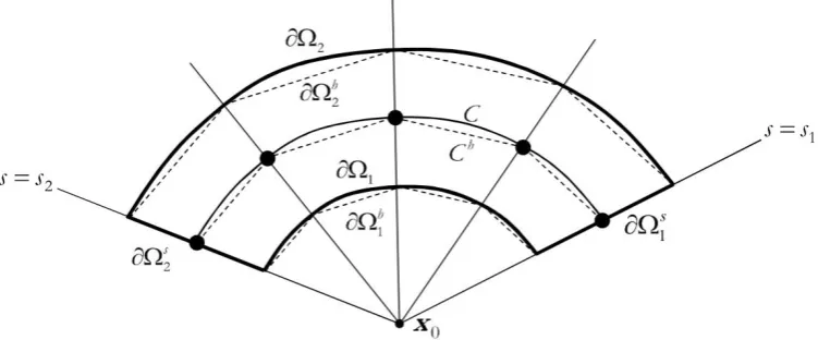
A set of scaled boundary finite element equations is established, here, for a generic, two-dimensional body as shown in Figure 4 to ensure that the resulting formulation is applicable to various cases. The boundary of the domain is assumed consisting of four parts resulting from the scale boundary coordinate transformation with the scaling center x0 and defining curve C : the inner boundary 1, the
outer boundary 2, the side-face-1 1
s
, and the side-face-2 2
s
. For certain special cases such as closed bodies without the side face, bodies containing the scaling center, and unbounded bodies, it simply takes 1 2
s s
, 1 , and 2 in the following formulation, respectively. The
approximation of the given body is achieved via the discretization of the defining curve Ch along with the mapping region [ , ] [ , ] 1 2 s s1 2 in the
s plane, and the approximate body is denoted byh
. In particular, the approximate inner and outer boundaries 1
h
and 2
h
, the side-face-1 1
s
, and the side-face-2 2
s
are fully described by a curve 1,s1 s s2, a curve 2,s1 s s2, a straight line
1, 1 2
s s , and a straight line s s 2, 1 2, respectively.
Fig. 4. Schematic of a generic body and its approximation h. The dashed lines are used to represent
[image:10.595.114.490.563.719.2]From the boundary partition 1 2 1 1
s s
and the coordinate transformation (15), the
weak-form equation (13) can be rewritten for this generic body as
2 2 2 2 2 2
1 1 1 1 1 1
2 2
1 1
1 1 1 2 2 2
1 1 1 2 2 2
( ) ( ) ( ) ( ) ( ) ( )
( ) ( ) ( ) ( )
s s s s
T T T s T s
s s s s
s T s s T s
J d ds J d ds s J s ds s J s ds
J d J d
Lw D Lu w b w t w t
w t w t
(35)
where w1, w2, 1
s
w , 2
s
w are restrictions of the weight function
w
on the boundaries 1, 2, 1s
,
2
s
, respectively; t1, t2, 1
s
t , 2
s
t are surface flux on the boundaries 1, 2, 1
s
, 2
s
, respectively; and J1 J s( )1
,
2 ( )2
J J s . Next, by introducing the approximations of the body flux (32) and the derivatives of the weight function (33) along with the domain approximation, the integral on the left-hand side of (35), denoted for convenience by I1, becomes
2 2 2 2
1 1 1 1
2 2 2 2
1 1 1 1
1 , 1 1 , , 1 2
2 1 , 2 2
( ) ( )
( ) ( )
s s
h T T h h h T T h h
s s
s s h
h T T h h h T T h
s s
J d ds J d ds
J
J d ds d ds
W B DB U W B DB U
W B DB U W B DB U
I
(36)
Further integrating the first two integrals by parts with respect to the coordinate and recalling that the matrices B1 and B2 are independent of the coordinate ,
h
W and Uh are independent of the coordinate
s, and the matrix
D
is independent of both and s, the integral I1 is simplified to
2
1
2 1
1 0 , 1 1 0 , 2
2 0 , 1 1 0 , 1
1
( ) ( )
( ) ( )
h T h T h h
h T h T h h T h T h
d
W E U E E E U E UW E U E U W E U E U
I
(37)
where 1 ( 1)
h h
W W , 2 ( 2)
h h
W W , and E0, E1, and E2are defined by 2
1
0 1 1
s
T h
s
J ds
E B DB ,
2
1
1 2 1
s
T h
s
J ds
E B DB ,
2
1
2 2 2
s
T h
s
J ds
E B DB (38)
It is evident that both matrices E0 and E2 are symmetric. By following a similar procedure, the boundary
integrals appearing on the right-hand side of (35), denoted by I2, can be approximated by
2
21 1
2 (W1h T) P1 (W2h T) P2 (Wh T) F1td (Wh T) F2td
I (39)
where 1 ( 1)
S S s s
N N , 2 ( 2)
S S s s
N N , and
2
1
1 ( ) 1( ) 1 ( )
s
S T sh
s
s J s ds
P N t ,
2
1
2 ( ) 2( ) 2 ( )
s
S T sh
s
s J s ds
P N t (40)
1 ( 1) 1( ) 1
t S T s Jh
F N t , 2t ( 2S T s) 2( ) J2h
in which 1 ( )1
h h
J J s and 2 ( )2
h h
J J s . Without loss of generality, the first and last nodes resulting from the discretization of opened bodies are taken as a node on the side-face-1 and a node on the side-face-2, respectively, and this applies in what follows. It should be remarked from the Kronecker property of the nodal basis functions that (1)( ) 1s1 , ( )j ( ) 0 s1 j 2 and ( )m ( ) 1s2 , ( )j ( ) 0 s2 j m 1. Now,
both the matrices N1S and N2S clearly contain many zero entries and simply take the form
1 { }
S
N I 0 0 , 2 { }
S
N 0 0 I (42)
Substituting (42) into (41) leads to
1t {J1h s1( ) }T
F t 0 0 , 2t { J2h s2( )}T
F 0 0 t (43)
where 0 is a zero -component vector. Finally, the domain integral associated with the distributed body source on the right-hand side of (35), denoted by I3, can be approximated by
2
1
3 ( h T) bd
W FI (44)
where the matrix
F
bis defined by2 2 2 2
1 1 1 1
(1) ( 2) ( )
( )
T
s s s s
b S T h h h h
m
s s s s
J ds J ds J ds J ds
F N b b b b (45)
By combing the results (37), (39) and (44), the approximation of the weak-form (35) becomes
2 12 1
0 , 1 1 0 , 2
2 0 , 1 2 1 0 , 1 1
1
( ) ( )
( ) ( ) 0
h T h T h h t b
h T h T h h T h T h
d
W E U E E E U E U F F
W E U E U P W E U E U P
(46)
where Ft F1t F2t. From the arbitrariness of the weight function Wh, it can be deduced that
2 2
0 , ( 0 1 1) , 2 ( , )1 2
h T h h t b
E U E E E U E U F F 0 (47)
1 1
( )
h
Q P (48)
2 2
( )
h
Q P (49)
where the vector
Q
h Q
h( )
known as the nodal internal flux is defined by0 , 1
( )
h h T h
Q E U E U (50)
condition (49) is ignored for unbounded bodies; the boundary condition (48) is ignored for bounded bodies containing the scaling center; the term
F
t vanishes for closed bodies; and the termF
b vanishes for bodiesfree of the distributed body source.
2.5.
Treatment of Prescribed Conditions on Side Faces
It should be evident from (47)-(49) that the information associated with the prescribed distributed body source and the prescribed boundary conditions on both inner and outer boundaries can be integrated into the formulation via the term Fb and the boundary conditions (48)-(49), respectively. However, the
consideration of the prescribed surface flux and state variable on the side face is still not apparent from the above formulation. The system of linear differential equations (47) can be further re-expressed in a form well-suited for the treatment of those prescribed side-face conditions.
First, bodies considered in the present study are divided into five groups, Group-1, Group-2, Group-3,
Group-4, and Group-5, associated with closed bodies without the side-face, opened bodies with prescribed
surface flux on both side faces, opened bodies with prescribed surface flux on the side-face-1 and prescribed state variable on the side-face-2, opened bodies with prescribed surface flux on the side-face-2 and prescribed state variable on the side-face-1, and opened bodies with prescribed state variable on both side faces, respectively. For bodies in Group-1, Uh contains only unknown functions and
1
s
t , 2
s
t disappear; for bodies in Group-2, Uh contains only unknown functions whereas
1
s
t , 2
s
t are fully prescribed; for bodies in Group-3, 1
s
t , and ( )( )
h
m
u are fully prescribed and 2
s
t and the remaining functions ( )( ) 1
h
i i m
u in
h
U are unknown; for bodies in Group-4, 2
s
t and (1)( )
h
u are fully prescribed and 1
s
t and the remaining functions u( )hi ( ) i 2 in Uh are unknown; and for bodies in Group-5, both u(1)h ( ) and u( )hm( ) are fully
prescribed whereas 1
s
t , 2
s
t , and the remaining functions ( )( ) 2 1
h
i i m
u in Uh are unknown. To
treat the prescribed conditions on the side-face for bodies in all groups, the vector Uh is partitioned and
rearranged into known and unknown parts as Uh {Uhu Uhc T} where Uhu Uhu( ) contains only
unknown functions from a collection u( )hi ( ), i 1, 2,...,m and Uhc Uhc( ) contains the remaining known
functions associated with the prescribed state variable on the side face. By defining as the number of known functions ( )( )
h
i
u contained in Uhc, the number of remaining unknown functions ( )( )
h
i
u contained in Uhu is therefore equal to m p . Clearly, the value of p associated with bodies in Group-1, Group-2,
Group-3, Group-4, and Group-5 are 0, 0, 1, 1, and 2 respectively. Consistent with the partition of the vector
h
U , the vector
F
t can be also partitioned into{ }
t tu tc T
F F F where
F
tu F
tu( )
contains many zero functions and known functions corresponding to the prescribed surface flux on the side face and( )
tc tc
F F contains unknown functions associated with the unknown surface flux on the side face. According to this partition, the system of differential equations (47) can be separated into
2 2
0 , 0 ( 1 ) 1 , 2
uu hu uu uu T uu hu uu hu tu bu suu
E U E E E U E U F F F (51)
2
tc bc suc scc
F F F F (52) where Fbu and Fbc results directly from the partition of the known vector Fb {Fbu Fbc T} and the
vectors Fsuu, Fscc and Fsucare defined by
2
0 , ( 0 ( 1 ) 1 ) , 2
suu uc hc uc cu T uc hc uc hc
F E U E E E U E U (53)
2
0 , 0 ( 1 ) 1 , 2
scc cc hc cc cc T cc hc cc hc
F E U E E E U E U (54)
2
0 , 0 1 1 , 2
( ) ( ) ( ) ( )
suc uc T hu uc T uc T cu hu uc T hu
F E U E E E U E U (55)
in which uu, uc, cu, cc
i i i i
E E E E for i0,1,2are sub-matrices resulting from the partition of the matrix Ei .
Note that both Fsuu and Fscc are known vectors obtained from the prescribed state variable on the side
face whereas Fsuc is given in terms of the unknown vector Uhu. By following the same procedure, the
relation (50) can be also partitioned into
0 , 1
( ) ( ) ( )
hu uu hu uu T hu huc
Q E U E U Q (56)
0 , 1
( ) ( ) ( ) ( )
hc uc T hu uc T hu hcc
Q E U E U Q (57)
where Qhuc( ) and Qhcc( ) are known vectors defined by
0 , 1
( ) ( )
huc uc hc cu T hc
Q E U E U , Qhcc( ) E U0cc ,hc (E1cc T) Uhc (58)
Now, a system of differential equations (51) together with the following two boundary conditions on the inner and outer boundaries (i.e., Qhu( )1 P1uand
2 2
( )
hu u
Q P ) is sufficient for determining the general solution Uhu of the given boundary value problem. Note that
1u
P and P2u are vectors resulting from the
partition of the vectors P1 and P2, respectively (i.e., P1{P1u P1c T} and P2{P2u P2c T} ). Once hu
U
is determined, the vectors Ftc,1
c
P , and P2c can be readily obtained.
3.
Solution Procedure
This section presents the procedure for obtaining the analytical solution of a system of linear, second-order, nonhomogeneous, ordinary differential equations (51) along with the prescribed conditions on both inner and outer boundaries. A corresponding eigenvalue problem is solved first to determine the homogeneous solution and the method of undetermined coefficients is then utilized to construct the particular solution associated with the distributed body source and the prescribed conditions on the side faces. Once the general solution is obtained, the boundary conditions on both inner and outer boundaries are enforced to determine all involved constants. Finally, the post-process for field quantities of interest such as the state variable and body flux is briefly described.
3.1. Determination of Homogeneous Solution
Following the standard procedure in the theory of differential equations, a homogeneous solution of a system of linear, second-order, Euler-Cauchy differential equations (51), denoted by U0hu , takes the
following form
2( ) 0
1
( ) i
m p
hu u
i i
i
c
U (59)
where i is termed the modal scaling factor, i is the (m p ) -component vector representing the ith
mode of the state variable, and c are arbitrary constants denoting the contribution of the ii th mode. The
nodal internal flux Q0hu( ) associated with
0
hu
U can be obtained as
2( ) 2( )
0 0 1
1 1
( ) i ( ) i
m p m p
hu uu uu T u u
i i i i i
i i
c c
Q E E q (60)
where u i
q is termed the ith modal internal flux defined in terms of u i
by
0 ( 1 )
u uu uu T u
i i i
By substituting (59) into (51) and then employing arbitrariness of c , it results in i
2
0 ( 1 ) 1 2 {1, 2,..., 2( ) }
uu uu T uu uu u
i i i i m p
E E E E 0 (62) By further rearranging terms in (61) such that
1 1
0 1 0
( ) ( ) ( )
u uu uu T u uu u
i i i i
E E E q (63) where 1
0
(Euu) denotes the inverse of
0uu
E , and then substituting this result into (62), it finally yields
1 1
2 1 ( 0 ) ( 1 ) 1 ( 0 )
u uu uu uu uu T u uu uu u
i i i i
q E E E E E E q (64)
Now, by introducing a 2(m p ) -component vector Xi such that { }
u u T
i i i
X q , equations (63) and (64) can be combined into a system of linear algebraic equations
i i i
AX X (65)
where a coefficient matrix A is given by
1 1
0 1 0
1 1
2 1 0 1 1 0
( ) ( ) ( )
( ) ( ) ( )
uu uu T uu
uu uu uu uu T uu uu
E E E
A
E E E E E E (66)
Determination of 2(m p ) pairs of { ,i Xi} can be achieved by solving the eigenvalue problem (65) where i denotes the eigenvalue and Xi are the associated eigenvector. It should be remarked that since
A is, in general, not symmetric, { ,i Xi} involves complex numbers. In fact, only a half of the eigenvalues has the positive real part whereas the other half has the negative real part. Let and be (m p ) (m p ) diagonal matrices containing eigenvalues with the positive and negative real parts, respectively, andqbe matrices whose columns are u
i
and u i
q of the eigenvector { u u T}
i i i
X q
associated with i in
, and and qbe matrices whose columns are u i
and u i
q of the eigenvector { u u T}
i i i
X q associated with i in
. Now, the homogeneous solutions U0hu and Q0hu( ) are given by
0hu( ) ( ) ( )
U C C (67)
0 ( ) ( ) ( )
hu q q
Q C C (68)
where and are diagonal matrices obtained by replacing the diagonal entries i of the matrices
and by a function i , respectively; and C and C are vectors containing arbitrary constants
representing the contribution of each mode. It is apparent that the diagonal entries of become infinite when whereas those of is unbounded when 0. As a result, C is taken to be 0 to ensure the boundedness of the solution for unbounded bodies and, similarly, the condition C 0 is enforced for bodies containing the scaling center.
3.2. Determination of Particular Solution
In the present study, the distributed body source b, the prescribed surface flux 1
s
t on the side-face-1, the prescribed surface flux t2s on the side-face-2, and the prescribed state variable Uhc on the side faces are
*
( , ) j ( )
j
j
s s
b b ,
*
1 1( )
j j s s j
t t ,
*
2 2( )
j j s s j
t t ,
*
( ) j j hc hc j
U U (69)
where * denotes a set of non-negative real numbers, ( )
j s
b are given vector-value functions, and s1
j
t ,
2
s j
t , hc j
U are given constant vectors. Substituting (69) into (43), (45) and (53) yields
* j j b b j
F F ,
* 1 1 j j t t j
F F ,
* 2 2 j j t t j
F F ,
* j j suu suu j
F F (70)
where b j
F , t1
j
F , t2
j
F , and suu j
F are constant vectors defined, in terms of prescribed data, by
2 2 2
1 1 1
(1) ( ) ( 2) ( ) ( ) ( )
T
s s s
b h h h
j j j m j
s s s
s J ds s J ds s J ds
F b b b (71)
1 1
1
{ }
t h s
j J j
F t 0 0 , 2 2
2
{ }
t h s T
j J j
F 0 0 t (72)
( 1) 0 ( 0 ( 1 ) 1 ) 2
suu uc uc cu T uc uc hc
j j j j j
F E E E E E U (73)
Based on this form of prescribed data and the method of undetermined coefficients, the particular solution of (51), denoted by 1
hu
U , takes the form
1 2
1 ( ) 1 ( ) 1 ( ) 1 ( ) 1 ( )
hu hub hut hut huu
U U U U U (74)
where
* 2 1 ( )
j j hub b j
U c ,
* 1
1 1
1 ( )
j j hut t j
U c ,
* 1
2 2
1 ( )
j j hut t j
U c ,
* 1 ( )
j j huu uc j
U c (75)
with b j
c , t1
j
c , t2
j
c , and uc j
c being vectors of unknown constants determined from the following four systems of linear algebraic equations
( 2)( 1) 0 ( 2) 0 ( 1 ) 1 2
uu uu uu T uu uu b bu
j j j j j
E E E E E c F 0 (76)
1 10 0 1 1 2
( 1) uu ( 1) uu ( uu T) uu uu t tu
j j j j j
E E E E E c F 0 (77)
2 20 0 1 1 2
( 1) uu ( 1) uu ( uu T) uu uu t tu
j j j j j
E E E E E c F 0 (78)
( 1) 0 ( 1) 0 ( 1 ) 1 2
uu uu uu T uu uu uc suu
j j j j j
E E E E E c F 0 (79) where bu
j
F , tu1
j
F and tu2
j
F result from the following partitions b { bu bc T}
j j j
F F F , t1 { tu1 tc1}T
j j j
F F F , and
2 { 2 2}
t tu tc T
j j j
F F F , respectively. Once the particular solution U1hu( ) is obtained, the corresponding
particular nodal internal flux, denoted by 1 ( )
hu
Q , is calculated from
1 ( ) 0 1, ( 1 ) 1
hu uu hu uu T hu
Q E U E U (80)
3.3. Final General Solution