Theses Thesis/Dissertation Collections
7-1-2013
Current sensing feedback for humanoid stability
Matthew DeCapua
Follow this and additional works at:http://scholarworks.rit.edu/theses
This Thesis is brought to you for free and open access by the Thesis/Dissertation Collections at RIT Scholar Works. It has been accepted for inclusion in Theses by an authorized administrator of RIT Scholar Works. For more information, please [email protected].
Recommended Citation
By
Matthew DeCapua
A Thesis Submitted
in
Partial Fulfillment
of the
Requirements for the Degree of
MASTER OF SCIENCE
in
Electrical Engineering
Approved by:
PROF__________________________________________________________ (Dr. Ferat Sahin, Thesis Advisor)
PROF__________________________________________________________ (Dr. Amuso, Thesis Committee Member)
PROF__________________________________________________________ (Dr. Phillips, Thesis Committee Member)
PROF__________________________________________________________ (Dr. Sohail A. Dianat, Department Head)
DEPARTMENT OF ELECTRICAL AND MICROELECTRONIC ENGINEERING
KATE GLEASON COLLEGE OF ENGINEERING
ROCHESTER INSTITUTE OF TECHNOLOGY
ROCHESTER, NEW YORK
Abstract
For humanoid robots to function in changing environments, they must be able to maintain
balance similar to human beings. At present, humanoids recover from pushes by the use of
either the ankles or hips and a rigid body. This method has been proven to work, but causes
excessive strain on the joints of the robot and does not maximize on the capabilities of a
humanlike body. The focus of this paper is to enable advanced dynamic balancing through
torque classification and balance improving positional changes.
For the robot to be able to balance dynamically, external torques must be determined
accurately. The proposed method of this paper uses current sensing feedback at the humanoids
power source to classify external torques. Through understanding the current draw of each joint,
an external torque can be modeled. After being modeled, the external torque can be nullified
with balancing techniques. Current sensing has the advantage that it adds detailed feedback
while requiring small adjustments to the robot. Also, current sensing minimizes additional
sensors, cost, and weight to the robot. Current sensing technology lies between the power supply
and drive motors, thus can be implement without altering the robot.
After an external torque has been modeled, the robot will undertake balancing positions
to reduce the instability. The specialized positions increase the robot’s balance while reducing
the workload of each joint. The balancing positions incorporate the humanlike body of the robot
and torque from each of the leg servos. The best balancing positions were generated with a
genetic algorithm and simulated in Webots. The simulation environment provided an accurate
physical model and physics engine. The genetic algorithm reduced the workload of searching
The current sensing theory was experimentally tested on the TigerBot, a humanoid
produced by the Rochester Institute of Technology (RIT). The TigerBot has twenty three
degrees of freedom that fully simulate human motion. The robot stands at thirty-one inches tall
and weighs close to nine pounds. The legs of the robot have six degrees of freedom per leg,
which fully mimics the human leg. The robot was awarded first place in the 2012 IEEE design
Table of Contents
I. List of Figures
II. List of Tables
III. Introduction
1.
Literature Review
1
1.1. Zero Moment Point Theory 1
1.2. Linear Inverse Pendulum Model 3
1.3. Proposed Balancing Techniques 6
1.4. Push Recovery Strategies 9
1.4.1 Ankle Strategy 10
1.4.2 Hip Strategy 10
1.4.3 Foot Placement and Stepping Strategy 11
1.5. Proposed Walking Techniques 13
2.
Theory of Current Sensing
18
2.1. Sagittal Torque Derivation due to Gravity 19
2.2. Coronal Torque Derivation due to Gravity 21
2.3. Current Sensing for Stability 23
2.3.1. Current’s Relation to Torque 24
2.3.2. Magnitude Estimation of Destabilizing Torque, Sagittal Plane 25
2.3.3. Magnitude Estimation of Destabilizing Torque, Coronal Plane 27
3.
Positional Estimation
29
3.1. Estimation of Sagittal External Torques 30
3.2. Estimation Coronal External Torques 32
3.3. Sagittal and Coronal Directional Disturbances 34
4.
Current Sensing Implementation
35
4.1. Current Sensing Integrated Circuit 36
4.2. Current Sensing Circuit 39
4.3. Current Sense Processing 42
4.4. Proof of Concept 43
5.
Forward Kinematics
44
6.
Inverse Kinematics
52
7.
TigerBot
60
7.1. Mechanical Design 61
7.1.1. Proportionate Layout 62
7.1.2. Torque Calculations 64
7.1.3. Stress Analysis 66
7.1.4. Servo Motor 66
7.2. Power Distribution 68
7.3. System Architecture 70
7.3.1. Roboard 71
7.3.2. Servo Controller SSC32 72
7.3.3. Gyroscope 73
7.3.4. Graphical User Interface 73
7.4. Overall Specifications 75
8.
Comparison of Research Humanoids
75
8.1. Robonova 76
8.2. DARwIn-OP 77
8.3. Nao 79
8.4. Conclusion 80
9.
Webots
81
9.1. Simulation Model 81
9.2. Simulation Programming 82
9.3. Simulation Application 83
10.
Genetic Algorithm
83
10.1. Genetic Algorithm Overview 84
10.2. Published Work for GA and Humanoids 86
10.3. Proposed GA 88
10.3.1. Genetic Algorithm Parameters 88
10.3.2. Fitness Function 89
10.3.3. Selection Criteria 90
10.3.4. Cross Over 90
10.4. MATLAB Implementation 91
11.
GA Produced Balancing Positions
96
11.1. Sagittal Positions 96
11.2. Coronal Positions 99
11.3. Combined Positions 100
11.4. Problems with Webots 101
12.
Experimental Implementation
101
12.1 Current Sensing IC Problem 102
12.2 Current Sensing Resistor Problem 104
12.3 Implementation 105
13. Experimental Results
106
13.1 Experimental Model 106
13.2 Experimental Sagittal Magnitude 108
13.2.1 Soft Sagittal Destabilizing Torque 109
13.2.2 Medium Sagittal Destabilizing Torque 111
13.3 Experimental Coronal Magnitude 112
13.3.1 Soft Coronal Destabilizing Torque 113
13.3.2 Medium Coronal Destabilizing Torque 114
13.4 Experimental Implementation of Position Estimation 115
13.4.1 Push at the R1 Position 117
13.4.2 Push at the R2 and R3 Positions 118
13.4.3 Push at the R4 and R6 Positions 119
13.4.4 Push at the R5 and R7 Positions 121
13.4.5 Push at the R9 and R10 Positions 122
13.4.6 Sagittal vs. Coronal 124
13.4.7 Weight Distribution Problems for Positional Estimation 124
13.4.8 Slipping Problems for Coronal Balancing 124
13.5 Experimental Balancing 125
13.5.1 Balancing Implementation 127
13.5.2 Balancing Results 128
13.5.3 Experimental Balancing Problems 129
14.
Current Sensing Advantages as a Feedback Control
130
14.1 Power Conservation 130
14.2 Feedback per Servo 132
14.3 Small and Simple Application 133
15.
Conclusion and Future Work
133
I.
List of Figures
Figure 1.1. Proposed Trajectory of Humanoid’s ZMP
Figure 1.2. Linear Inverse Pendulum Model
Figure 2.1. Sagittal Plane of Humanoid
Figure 2.2. Coronal Plane of Humanoid
Figure 2.3. External Torques Applied to Robot
Figure 3.1. Sagittal Applied Forces on Robot
Figure 3.2. Coronal Applied Forces on Robot
Figure 3.3. Angular Disturbance
Figure 4.1. INA196 Pin-out [19]
Figure 4.2. Gain Plot of INA196 [19]
Figure 4.3. INA196 Current Sensing Shunt [19]
Figure 4.4. Schematic for Current Sensing
Figure 4.5. Implementation of Current Sensing PCB
Figure 4.6a. Top Layer of Current Sense PCB
Figure 4.6b. Bottom Layer of Current Sense PCB
Figure 4.7. Arduino Mega 2560
Figure 4.8. Experimental PCB
Figure 4.9. Linear Output Range of IC Chip Compared with Differential Voltage
Figure 7.1. TigerBot
Figure 7.2. TigerBot Body Design
Figure 7.3. Custom Designed Hip Joint
Figure 7.4. TigerBot Leg Assembly
Figure 7.5. Mechanical Torque for Varied Positions
Figure 7.6. Stress Analysis of Custom Bracket
Figure 7.7. Roboard RS-1270
Figure 7.9. System Configuration
Figure 7.10. Roboard 110 [34]
Figure 7.11. SSC32 Servo Controller [33]
Figure 7.12. Gyroscope and Accelerometer
Figure 7.13. Graphical User Interface
Figure 8.1. Robonova [39]
Figure 8.2. DARwIn-OP
Figure 8.3. Nao [43]
Figure 9.1. TigerBot Model in Webots
Figure 10.1. Chromosome
Figure 10.2. Population
Figure 10.3. Matrix of Random Numbers for Parent Selection
Figure 10.4. Matrix of Fitness Values
Figure 10.5. Generated Mask
Figure 10.6. Transformed Mask
Figure 10.7. Parent Selection Mask
Figure 10.8. Two Point Crossover Mask
Figure 11.1. Torque Applied in Front
Figure 11.2. Torque Applied in Front
Figure 11.3. Torque Applied in Coronal Direction
Figure 11.4. Torque Applied in Both Directions
Figure 12.1. Low Pass Filter
Figure 12.2. Small Current Draw
Figure 12.3. Medium Current Draw
Figure 12.4. Large Current Draw
Figure 13.1a. Experimental Model
Figure 13.2. Soft Chest Hit Joint Currents
Figure 13.3. Soft Chest Hit Current Draw
Figure 13.4. Medium Chest Hit Joint Currents
Figure 13.5.Medium Chest Hit Current Draw
Figure 13.6. Servo Currents for Soft Torque
Figure 13.7. Summed Coronal Currents
Figure 13.8. Joint Currents
Figure 13.9. Summed Currents
Figure 13.10. Positional Estimation
Figure 13.11. R1 Current Values
Figure 13.13. R2 Current Values
Figure 13.14. R4 Current Values
Figure 13.15. R6 Current Values
Figure 13.16. R5 Current Values
Figure 13.17. R7 Current Values
Figure 13.18. Coronal Shoulder Torque
Figure 13.19. Coronal Knee Torque
Figure 13.20. Coronal Shoulder Torque, Opposite Direction
Figure 14.1. Standing High Power Consumption
II.
List of Tables
Table 5.1. DH-Table for Figure 9
Table 7.1. Torque Calculations
Table 7.2. Catalog Data for RS-1270
Table 7.3. TigerBot Specifications
Table 8.1. Robonova Specifications [39],[40]
Table 8.2. DARwIn-OP Specifications [41]
Table 8.3. Nao Specifications [42]
Table 10.1. GA Parameters
Table 10.2. Average Fitness of Function 1
Table 10.3. Average Fitness of Function 2
Table 10.4. Average Fitness of Function 3
Table 10.5. Average Fitness of Function 4
Table 10.6. Average Fitness of Function 5
Table 10.7. Average Fitness of Function 6
III.
Introduction
Humanoid robots have become a large area of focus in the field of robotics. A robot is
classified as a humanoid when it mimics the appearance and locomotion of a human being.
These kinds of robots are important for research into human motion and have the potential of
being used for dangerous or mundane jobs. Private companies and research facilities have begun
developing humanoids that range from a few inches tall to human height. A humanoid robot
uses bipedal motion for movement, thus it is subjected to large instabilities and complex
movements. The main focus of humanoid research has been implementing stability in balancing,
push recovery, and walking.
Present day research has produced several theoretical models for generating a stable
humanoid robot. The main theories used for humanoid balancing included zero moment point,
control of the robot’s center of gravity, an inverted pendulum model, and advanced inverse
kinematics. These methods have been explained in detail in the literature review.
The proposed theory presented in this paper utilizes a combination of sensor feedback to
enable stable balancing and push recovery. The main focus of the paper is implementing current
sensing as a feedback for producing balance control. The feedback from the current sensors is
combined with balancing positions generated by a genetic algorithm to facilitate push recovery.
This paper presents several sections that portray an in-depth analysis of current sensing,
balancing positions, humanoids, and push recovery. Section 1 presents a literature review of
humanoid research. The literature review discusses zero moment point theory, the linear inverse
pendulum model, balancing a humanoid robot, push recovery strategies, and walking research.
balancing. Current sensing was derived for each of the leg servos and relates to the
destabilization of the robot. Section 3 discusses how current sensing can be used for determining
the position of an applied external torque. Positional estimation is necessary for determining
how a robot should balance given a random push. Section 4 describes the hardware
implementation of the proposed current sensing theory.
Section 5 derives the forward kinematics of a humanoid robot. Forward kinematics are
important for the control of a robot and for determining the effect of each joint on the position
and orientation of its foot. Section 6 presents an in-depth derivation of the inverse kinematics of
a humanoid. Inverse kinematics are important for determining the effect of the foot’s position
and orientation on the joints of the robot. Inverse kinematics are also important for generating
balancing positions for the robot. Section 7 depicts the experimental robot used for testing the
current theory. The TigerBot’s design and specification are discussed in great depth. Section 8
discusses other available research humanoids as a benchmark for the TigerBot. This section
ensures that the TigerBot is a viable research platform as compared to other research models.
Section 9 presents the simulation program Webots. This simulation program was used to
generate the balancing positions in place of iterative experimental testing. Section 10 presents
the genetic algorithm used to generate the balancing positions. Section 11 shows the balancing
positions generated by the genetic algorithm. Section 12 discusses the experimental
implementation of the current sensing hardware on the TigerBot and the problems that occurred.
Section 13 discusses the experimental results of the current sensing based balancing and
positional estimation. Section 14 presents a few advantages of current sensing over other
1
1.
Literature Review
Humanoid research reveals a variety of methods to implement balancing, push recovery,
and stable walking. The published works presented Zero Moment Point (ZMP) as the most
commonly used guideline for ensuring stable motion. ZMP ensures stability by keeping the
moment of the robot’s forces within the geometry of the feet. The Linear Inverse Pendulum
Model (LIPM) was shown to being the most commonly used modeling system for a humanoid
robot. A LIPM simplifies the dynamics of a humanoid and leads to stable locomotion by
maintaining control over the robots center of gravity (COG). LIPM and ZMP tend to be
combined when generating control laws for motion. The presented sections for the literature
review are as follows: a discussion of ZMP and LIPM, a review of other published balancing
techniques, a summary of push recovery strategies, and a report of a variety of methods for stable
walking.
1.1. Zero Moment Point Theory
Zero Moment Point theory has been the primary method for ensuring stability in a
humanoid for almost two decades [23]. The theory of ZMP was first proposed by Vukobratovic
[24] in his paper written in 1990. Over the past twenty years, his novel theory has been
implemented in most humanoid research projects [5] [7] [8] [13-17] [18] [20] [21] [23-27].
ZMP focuses on implementing dynamic balancing by ensuring that the moment of the forces of
the robot remains within the robot’s foot [25]. Thus, the contact forces from the robot are
canceled by the ground’s reaction force. The theory of ZMP is well described in a reference
2 For a robot to remain stable, its ZMP must remain within the geometry of its foot. Figure
1.1 demonstrates a proposed trajectory for a robot’s foot while walking. Walking was chosen for
demonstration purposes because it shows an extreme case of instability. The red line in Figure
1.1 shows how the ZMP must remain within the sole of the robot throughout the entire motion.
The trajectory of the robot must also focus on keeping the center of gravity of the robot between
the two feet, which is shown with the green line.
Figure 1.1. Proposed Trajectory of Humanoid’s ZMP
Humanoid stability is also complicated by the single and double support phases.
Throughout the motion of the robot, it can have either of its feet on the ground or both. Thus, the
ZMP criteria must be applicable in both cases. The dark grey region of Figure 1.1 demonstrates
the safe region of the foot for the single support phase of the walking algorithm. The light grey
region shows the safe region for the double support phase of the humanoid motion [18]. The
ZMP of a robot can be difficult to maintain and changes throughout any motion, thus additional
controllers are required for implementation.
The position of the ZMP for a robot can be calculated with the use of the equations [18]
below.
∑ (
)
∑
3
∑ ( ) ∑
∑ (1.2)
The above equations demonstrate how the location of the ZMP is dependent on the
position of the robot. The ZMP calculations take into account the effect of each link of the robot,
starting from the first to the . The mass of the robot and its links are accounted for with the
term. The position of the center of mass (COM) of each link are represented with the
variables , and . The resulting values for the and must remain within the
positions show in Figure 1.1 for the robot to remain stable. If the position of the ZMP moves
outside of the foot’s geometry, then advanced control systems are required to return it to the
proper position. This method for determining the robot’s present ZMP can be very
computationally heavy. Research shows that controllers focused only on controlling a robot’s
ZMP can produce results that increase stability. ZMP theory is the same for balancing and push
recovery.
1.2. Linear Inverse Pendulum Model
ZMP has been presented as the main method for ensuring stability in humanoid robots.
However, this criterion does not assist with modeling the robot or implementing dynamic
motion. A humanoid has numerous degrees of freedom which makes modeling very
complicated. Thus, most research uses the simplified model of a Linear Inverse Pendulum for a
humanoid [1-4] [8] [10] [15] [20] [21]. The body of the humanoid is abstracted into a single
mass point as a model of its COM [3]. In the following derivations, center of mass and center of
gravity are used interchangeably due to a humanoid’s limited height. Due to the cyclical nature
4 pivot of the pendulum occurs at the feet, thus the modeling is considered an inverse pendulum.
Figure 1.2 demonstrates an abstraction of a humanoid robot with the use of a LIPM.
Figure 1.2. Linear Inverse Pendulum Model
This extreme simplification removes the complexities of numerous degrees of freedom
and obscure body geometry. Some research investigates adding additional aspects of humanoids
to the model to create better accuracy but more difficult modeling. The LIPM model can be
improved by accounting for joint friction, unknown reaction forces, body complexities, and
offsets associated with a miscalculated COM position.
The above figure can be used to derive control for a humanoid. To ensure that the robot
is stable while moving, the motion of the center of gravity is controlled. The motion of the
center of gravity of the robot is affected by gravity and the contractility of the robot. This fact
enables for the derivation of the robot’s kinematic equations [3]. By analyzing the free-body
diagram of the robot’s COG, the following equation can be derived.
(1.3)
5
(1.4)
Thus,
(1.5)
Where x is the horizontal position of the center of gravity and is the height of the
robot’s center of gravity. Through solving the above differential equation, a kinematic equation
of the center of gravity of the robot can be derived.
( ) ( ) (1.6)
( ) (1.7)
where √
The above equation expresses the trajectory of a humanoid’s center of gravity that has
been modeled based on a Linear Inverse Pendulum. Equation 1.6 models the position of the
center of gravity as it moves over time. Equation 1.7 demonstrates how the velocity of the center
of gravity changes over time. The equations are dependent on the initial horizontal position and
initial velocity. If the center of gravity remains within the above constrictions, then the robot can
move with stability. The presented method assumes that the center of gravity remains within the
same vertical position. More advanced LIP models account for the change in the vertical
position. As can be seen, the LIP model simplifies the calculation process significantly.
However, these simplifications can be difficult to apply to an experimental robot and do not
6
1.3 Proposed Balancing Techniques
Humanoids have the potential of being a large influence in society. The robots are
designed to mimic humans so as to be easier for society to accept and able to operate in a human
based environment. However, the natural figure of a humanoid robot is extremely unstable. For
the robot to function in society, it must be able to balance itself similar to humans. There has
been a lot of research conducted over the past decade in new ways to implement advanced
methods for balancing.
S. Lim et al. [5] presented a control algorithm for balancing humanoids that utilizes a
Zero Moment Point position feedback. The method requires fast determination of the robot’s
ZMP and uses that as a feedback control. The ZMP is extrapolated to a compensation angle that
can be added to the control of the robot to increase stability while not disturbing motion. The
angle was derived from applying Newton’s laws to the model of the robot. The MHR-1
humanoid was used for experimental testing. The results demonstrated a decrease in recovery
time when an instability disturbance was applied to the robot. The presented method shows that
monitoring the ZMP position can be used for balancing.
Seung-Joon Yi et al. [4] generated an active stabilization algorithm for a humanoid robot
undergoing impact motions with unknown reaction forces. The algorithm utilized dynamic
motion for balancing rather than static solutions. Thus, rotational motion at the joints was used
to counter act the unknown reaction forces. Their research focused on enabling humanoids to
generate larger torques for lifting heavy objects while maintaining balance. The larger balancing
torques was generated by using impaction verses quasi-static motions. The DARwIn-OP
humanoid was used for testing in both simulation and hardware. The implementation of testing
7 caused for instability from the punch’s reaction force. However, the testing did not thoroughly
investigate all possible instabilities. The balance recovery algorithm maintained the robots
stability for each of the varying weights in both hardware and simulation. The results
demonstrate the advantages of dynamic balancing over static.
Wei Xu et al. [28] implemented torque based compliance control for a humanoid robot to
compensate for impact forces of a landing foot. The control method was designed to absorb the
impact forces generated between the robot’s contacting foot and the ground. Reducing the large
impact force of stepping can be used to help keep the robot stable. A gait designed based on the
parameters of a LIPM was used to test the control algorithm. The employed controller modifies
the predetermined walking algorithm to absorb the impact force of the foot. The KONG-I
humanoid was used for experimental trials. The robot has force sensing circuitry on each foot to
determine the impact forces. The experimental results demonstrated a reduction in the impact
force. These results enable for additional stability to be present in the robot’s motion.
Kenji Kaneko et al. [29] discussed a method for estimating external forces acting on
humanoid robots. They argue that external force detection is a necessity for humanoids to
function in society. The method proposed coupled force sensors on each foot with an IMU
inside the robot’s cavity. The applied forces were estimated by comparing the reaction forces of
each foot with the ground. The reaction forces coupled with the IMU output determined the
position of the applied force. The HRP-2 humanoid was used for experimental testing. The
experimental test focused only on determining the applied forces. Additional control over the
robot was not implemented. Forces were applied to the robot’s wrist. The force detectors on the
wrist were compared with the output of the proposed method. Their method demonstrated force
8 Guocai Liu et al. [6] introduced a method for controlling a humanoid with dynamic
balancing. The dynamic balancing was implemented by controlling the robot’s stance leg length
and selecting suitable swing directions. A finite-state machine control system executed specified
actions in different stages of the walking motion to improve stability. While ensuring these
stages were met, their control algorithm maintained the body’s attitude, forward speed, and
swing leg angle. Their method was tested in MATLAB under several conditions of humanoid
motion. The humanoid model used for testing did not accurately represent a human body or
human motion. The feet were modeled with linear actuators rather than rotational joints. The
results demonstrated that the dynamic balance improved stability with the additional
disturbances of uneven ground, velocity changes, and walking on a ramp.
Joohyung Kim et al. [7] discussed controlling the balance of a biped robot through a
combination of gravity compensation, virtual gravity control, and damping control. The method
focused on using torque control to implement balance stability. The algorithm added a virtual
gravity control to compensate for the unknown balance disturbances. The virtual gravity control
was added to the ZMP model so it functioned within the boundaries of the ZMP theory. The
proposed model also accounted for the joint friction to further its accuracy. The Roboray
humanoid was used for experimental testing. The results demonstrated the robot balancing on
one and two legs. The experimental testing was conducted with small external forces. The
results showed that torque control can be used for advanced balancing and that increased model
accuracy provides better stability.
Benjamin J. Stephens et al. [1] presented an approach to balancing that utilizes the use of
force control. His method aimed at improving common balancing techniques by generating a
9 determining the necessary joint torques that will increase its stability. The torque control also
enabled for the contact forces of the robot to be improved. The Sarcos Primus humanoid was
used for experimental testing. The experimental testing was conducted through lifting a heavy
bucket that would vary in weight. This process simulated balance changes but did not
thoroughly address all possible instabilities. The experimental results demonstrated that the
robot maintained its balance when the additional controller was actively running. Thus,
monitoring torques was shown as a viable method for improving stability in a robot.
Benjamin J. Stephens [10] discussed a method using state estimation for force-controlled
humanoid balance using simple models in the presence of modeling error. The Linear Inverted
Pendulum model was used for generating the balancing dynamics. The method presented
focused on exploring the effects of unknown errors on balancing. The unknown center of mass
offset and external forces were focused on. These unknowns were added to the balance model as
variables. The balancing model was used to estimate the state of the robot and enable stability
improving control. The Sarcos Primus humanoid was used for experimental testing. The results
demonstrated that it is possible to determine the COM offset and external forces, which enabled
for better balance algorithms. However, it was difficult to estimate the external disturbances
while maintaining the proper states. The presented method showed force controlled balancing
can improved upon with accounting for more unknowns.
1.4 Push Recovery Strategies
For humanoids to become part of society, their balancing must be able to account for
unknown disturbances. Whether it is from human contact or contact with a stationary object,
human beings commonly must balance when experiencing a push. Thus, present day research
10 balance recovery after experiencing a push are the ankle strategy, hip strategy, and stepping
strategy [8].
1.4.1 Ankle Strategy
The ankle strategy implements push recovery by increasing the torque of the ankle joint
to counteract the forces due to a push [8]. This method is limited by the torque of the ankle, thus
is used for small applied torques.
Akash et al. [3] discussed a technique for implementing humanoid push recovery by
using theory derived from an advanced inverse pendulum model. The inverse pendulum model
used a three mass system to better model the motion of the robot. The equations of motion
derived from the pendulum model were used to design the ankle push recovery protocol. The
recovery method was designed for the geometric constraints of the Hoap-2 humanoid. The push
recovery model was tested in simulation through the use of Webots and varying push forces.
The results demonstrated control over the robot’s COM for forces that were under 12N.
However, the control algorithm was limited by larger forces, thus demonstrating the restrictions
of the method and ankle recovery. The results do demonstrate that the ankle strategy can
function properly for small forces and that additional controllers can be used to improve its
recovery ability.
1.4.2 Hip Strategy
The hip strategy implements push recovery by increasing the torque of the hip joint to
counteract forces due to a push. The torque of the hip is exerted closer to the COM of the robot,
thus generates a larger reaction force [8]. The hip strategy can produce larger counter forces so it
11 Dragomir Nenchev et al. [31] presented results for experimentally testing the validity of
the hip and ankle recovery strategies. The paper demonstrated derived theory for implementing
both of the recovery strategies. The theory was derived from the kinematics modeled with a
Linear Inverse Pendulum combined with a damping spring factor. The Hoap-2 was used to
experimentally test both recovery methods. The two methods were chosen from the impact data
collected by the acceleration sensor embedded in the chest of the robot. The results show the
constraints of both recovery strategies. The ankle recovery was viable for small forces but failed
after a certain threshold. The hip recovery was viable for larger forces than the ankle recovery
and had a fast recovery time. The experimental results show the strength and weaknesses of both
methods.
1.4.3 Foot Placement and Stepping Strategy
The stepping strategy implements push recovery by increasing the kinetic energy of the
robot to counteract the forces of a push. The robot steps towards the push so the applied force is
absorbed by the impact of the swinging leg [8]. This method enables for recovery from larger
pushes than the hip strategy, however it changes the motion of the robot.
Awais Yasin et al. [8] discussed implementing push recovery through foot placement.
The method implements balance recovery by using a step that can change in both direction and
step size. The specialized step size can increase the base of support for the robot undertaking a
variety of forces. The method was designed for use when applied forces were too large for use
of the hip or ankle recovery strategy. The characteristics of the step were estimated through an
inverse pendulum model coupled with the change in energy due to an external push. An Attitude
12 results demonstrated an increased ability to recover from large disturbances by using specialized
steps.
Wentao Mao et al. [11] presented a method for push recovery by using continuous steps.
The paper discussed the robot taking several continuous steps to balance from large disturbances.
The step size and number of steps was determined by the size of the exerted force. The motion
of the continuous steps was modeled with the use of a Linear Inverse Pendulum model. The
algorithm was designed for implementation on a robot with legs, a torso, but no arms. The
algorithm was tested in a simulator programmed by MFC of Visual Studio in conjunction with
the ODE physics engine. The results demonstrated that taking several continuous steps enabled
the robot to balance after enduring large external forces. The results also demonstrated that
increasing the step count enabled increased stability for larger forces.
Van Huan Dau et al. [15] implemented a method for humanoid push recovery while
maintaining the same walking scheme. The method enabled push recovery by modifying the
phase of the walking algorithm. Webots was used for testing in simulation with a human sized
robot. The use of the push recovery method was determined by detecting the change in orbital
energy at the robot’s center of mass. The recovery method was designed around two stages of
walking, which were called the acceleration and deceleration phases. The acceleration phase
occurred when the robot first stepped. The deceleration phase occurred when the robot was
landing at the end of stepping. The push recovery method was based on changing the phase of
the walking scheme during the deceleration phase. The robot continuously changed its phase
until balance was restored. The simulation results demonstrated successful balance recovery.
13 Shahram Jafari et al. [2] discussed implementing push recovery by using the knee joint.
The proposed method was implemented to demonstrate how the knee joint should also be
considered in push recovery. The three common methods of push recovery treat the knee as
stationary and do not account for its ability to assist. The knee strategy proposed was derived
from motion modeled with a linear inverse pendulum. The proposed method used additional
mathematical methods to create a more accurate balance stabilization technique. The results
demonstrated some improvement in the capabilities of the robot to recover its balance. However,
the results did not show significant improvement and were not tested experimentally. Also, the
simulation model was only six inches tall and does not pertain to most present day humanoid
robots.
Jiuguang Wang [9] discussed a method for humanoid push recovery by using robust
convex synthesis. A technique called sum-of-squares optimization automatically searched for
Lyapuov functions to improve the stability of nonlinear dynamic systems. This method enabled
them to simultaneously search for a balance controller and the domain in which the robot can
remain stable. They used their robust convex optimization to design a nonlinear feedback
control law to enable push recovery. The controller derived by their convex optimization was
tested through simulation with the LMI design toolbox YALMIP. The results collected through
simulation demonstrated that the model was able to balance while operating within possible
torques. The results were not tested experimentally but performed well in simulation.
1.5 Proposed Walking Techniques
Research into humanoid robotics focuses largely on generating stable walking
algorithms. A stationary robot with no lower extremities has been developed and implemented
14 to move, the motion dynamics become extremely complex and require very intricate control
systems. The main focus in research has been generating versatile and stable walking algorithms
that will enable humanoids to function in society.
Hsin-Yu Liu et al. [18] presented a course in simulation and demonstration of humanoid
motion for present day robots. The paper discussed how to control the stability of a robot
through the use of feedback and ZMP theory. The discussion of ZMP demonstrated the basic
equations that enable humanoid stability. The ZMP equations take a summation of the mass of
each limb and determine the position required for stability. Also, the paper demonstrated that the
ZMP of the robot must start at the foot and remain there when stationary. As the robot steps, the
ZMP must be in between the initial step and final step. Thus, the COM of the body must remain
between the two feet until the robot reaches placement of the second foot. The position of the
foot must be changed if the ZMP leaves the accepted region of stabilization. The paper proposed
that the foot position should be changed by the ankle to return the ZMP’s position to the stable
region. The paper also discussed that the knee and hip angle should remain the same to ensure
that the body is perpendicular to gravity at all times. These listed restrictions simplify balancing
but reduce the possible operation of a humanoid.
Ting Wang et al. [27] discussed an advance method for implementing stable gait in
humanoids. The method used a new control law by regulating the zero moment point and joint
path of the robot. Two positions of the robot’s ZMP are monitored throughout the motion. Also,
any unexpected rotations in the ankle were removed by the control system. The design is novel
in that it tracks the motion of the joints in the joint space rather than in a general reference path
15 demonstrated that the control law added stability throughout the walking process. The method
was not tested experimentally.
Fei Wang et al. [20] implemented gait planning based on the linear inverted pendulum
model for the Nao humanoid. The design of the step size and period were based on the structure
of the Nao robot. The method demonstrates an in-depth analysis of implementing humanoid
walking with ZMP theory and a LIPM. The results were tested in simulation and demonstrated
that these design methods produce stable walking.
Jun Morimoto et al. [12] proposed a biologically inspired biped locomotion strategy. The
kinematic dynamics of the robot were derived from the inverted pendulum model. The method
used the center of pressure of the robot to detect the phase of the inverted pendulum dynamics of
the humanoid motion. Force sensors on the feet of the robot were used to determine the robot’s
center of pressure and its velocity. The simplified gait trajectories were based on basic
sinusoidal functions. A coupled phase oscillator was used to synchronize the sinusoidal
functions with the phase detection. The frequency of the controller was proposed to be the
natural frequency of a linear pendulum to provide the best results. The horizontal motion of the
robot was controlled by sinusoidal motion at the hip and ankle. The vertical motion of the robot
was controlled by a sinusoidal motion at the hip, knee, and ankle. The results showed a basic
biped figure generating a stepping motion in simulation. Their method demonstrated successful
experimental trials for robots of several sizes. The experimental trials showed that biologically
inspired sinusoidal motion can be utilized to generate a stable walking algorithm.
Przemyslaw Kryczka et al. [13] discussed a method for humanoid walking through using
16 kinematics methodology to enable more human like gait through stretched knees. The algorithm
had been simplified to remove redundant calculations and improve computational difficulties.
Webots was used for simulation trials before experimental testing. The WABIAN-2R humanoid
was used for experimental trials. The robot has been designed with thirty-seven degrees of
freedom (DOF) and has a specialized foot to simulate human motion. The experimental results
demonstrated that a gait based on a stretched knee and heel-contact to toe-off phases can be
stable.
Changjiu Zhou et al. [14] presented a method that generated dynamically stable gait
planning for a humanoid climbing a sloped surface. The method focused on implementing
trajectories based on the zero moment point of the robot. The constraints implemented on the
algorithm were based on the stabilization criteria proposed by ZMP theory. To ensure smooth
transition for the stepping motion, the motion of the robot’s center of mass was controlled. The
method was designed around the motion constraints limited by the geometry of each limb. The
design process also focused on ensuring that the foot cleared the ground at all points of motion to
ensure that accidental contact did not interfere. The design process was broken up into single
foot and double foot stages. Also, the gait was designed to have the same initial and final
velocities and positions. The RoboErectus was used for experimental testing. The results
showed successful experimental trials and simulations for a robot walking on an inclined surface.
Daniel Lee et al. [16] discussed a practical method for bipedal walking on uneven terrain
by using surface learning and push recovery. The method used onboard sensors to determine the
inclination of the terrain and an online learning algorithm to learn the layout. The perturbations
caused by the uneven surface were corrected for with common push recovery methods. Webots
17 on the commercially available DARwIn-OP. The results demonstrated the method functioning
properly for the small inclinations that were tested.
Darwin Caldwell [21] proposed generating walking trajectory for humanoids modeled
with compliant joints. Compliant joints could improve walking by removing the negative effects
caused by having stiff legs. The walking algorithm focused on the center of mass of the robot
remaining in a stable location. The method was tested under the conditions of constant gait
frequency, modified gait frequency, and a load disturbance. The COMAN humanoid was used
for experimental testing. The results demonstrated that the robot was able to walk under the test
conditions. However, the walking algorithm showed deterioration in joint tracking precision and
ZMP tracking throughout the process.
Bokman Lim et al. [22] discussed implementing optimal gait primitives for dynamic
bipedal locomotion. The locomotion was implemented by using parametric gait primitives,
utilizing state-dependent torque control, and numerical optimization that accounted for
non-constant forces. The gait dynamically changed by parsing together primitive motions after
interpreting the best way to avoid instabilities effecting the robot. The dynamic gait enabled for
power efficiency to be increased by not requiring stiff legs. The Roboray humanoid was used for
experimental testing. The results demonstrate stable walking with the ability to walk straight or
on a curve.
Xiaojun Zhao et al. [17] presented a method for generating humanoid kinematics by
linking similarities based on human motion capture. The paper focused on developing a method
for more human like motion by mimicking captured human motion. The captured motion was
18 testing. The human motion was collected through a high frame rate camera and several markers
on a test subject. The stability criterion of ZMP theory was used in conduction with the collected
images. The experimental results demonstrated that the robot was able to follow the human’s
motion, but did not implement stable walking.
The next section presents an in-depth derivation of current sensing as it pertains to
balancing a humanoid robot. The theory presented is used as the core driving point of the
balancing feedback experimentally implemented.
2.
Theory of Current Sensing
The main focus of this paper is to implement advanced balance for humanoids. Research
has shown that controlling the stability of the center of mass of the robot is necessary for
maintaining balance. The proposed method controls the center of mass of the robot through
current sensing. The current of a servo motor can be correlated to its output torque, which can be
related to stability. Thus, the theory of how each servo’s current pertains to the torques applied
to the servo is required. A robot will always be under the effect of gravity, thus an in-depth
derivation of the effect of gravity is required for the control feedback. There are three body
planes for the human body: sagittal, coronal, and transverse. A sagittal torque is applied to the
front or back of a robot. A coronal torque is applied to the sides. The two transverse plane
servos in the hip are assumed to be fixed because they do not affect the robot’s stability, rather
its ability to turn. The presented sections are as follows: derivation of sagittal torque due to
19
2.1. SagittalTorque Derivation due to Gravity
The derivation of the destabilizing torque due to gravity at each sagittal servo is required.
The torques for the ankle, knee, and hip servo are derived below. The torque analysis requires
the weight and angle of the components involved. The weight of a humanoid is constant and the
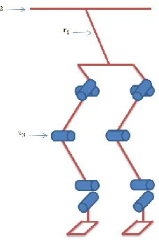
angles can be calculated from inverse kinematics. Figure 2.1 shows the labeling of the robot’s
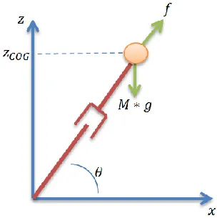
components that are important for sagittal torque. The robot is squatting because the position
[image:32.612.262.349.277.495.2]best demonstrates the torques applied to each servo.
Figure 2.1. Sagittal Plane of Humanoid
First, the torque of the ankle is derived. Torque analysis accounts for the weight of each
component of the robot. The terms account for the link length of the legs. The terms
account for the weight of a servo. The weight of the center of mass of the robot is assumed to
be split between the two legs for simplification.
( )
20
(2.1)
The weight and link length of the robot remain constant throughout operation. Thus, the
torque can be considered a constant multiplied by the angle of the joint.
; (2.2)
The torque of the knee joint has a similar derivation as the ankle, however only the
weight above the knee needs to be accounted for.
(2.3)
As can be seen in Equation 2.3, the angle of the knee is the only variable in the torque
analysis. Thus, the knee torque can be considered a constant multiplied by the angle of the joint.
(2.4)
The torque of the hip can be derived similar to the ankle and knee, but with only
accounting for the weight above the hip.
(2.5)
Similar to the other torques, the hip torque can be considered a constant multiplied by the
angle of the joint.
21 The above derivation shows how each servo’s torque due to gravity relates to the robot’s
geometry. The torque equations are the same for the left and right side because of the symmetry
of a humanoid.
2.2. CoronalTorque Derivation due to Gravity
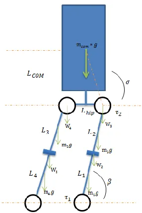
The derivation of the applied torque due to gravity at each coronal servo is required. The
torques for the rotation servos at the ankle and hip are derived. The torque analysis requires the
weight, link length, and angle of each component involved. Figure 2.2 shows the labeling of the
coronal perspective of the robot. The figure shows the robot standing on both legs while leaning
[image:34.612.233.376.342.556.2]to one side to better demonstrate the effect of gravity.
Figure 2.2. Coronal Plane of Humanoid
The torque for the right ankle was derived first. The weight of the COM of the robot is
22
( ) (
) (2.7)
The rotational torque at the ankle can be simplified to constant geometric values
multiplied by the angle of rotation.
( ) (
) (2.8)
The torque for the right hip was derived next. The torque at the hip also splits the COM
between the two legs for simplification.
(
) (2.9)
The rotational torque at the hip can be simplified to constant geometric values multiplied
by the angle of rotation.
(
) (2.10)
The torque for the left ankle was derived next. The left ankle has similar results as the
right ankle because the components of the humanoid are matched.
( ) (
) (2.11)
The rotational torque at the ankle can be simplified to constant geometric values
23
( ) (
) (2.12)
The torque for the left hip was derived next. The torque at the hip also splits the COM
between the two legs for simplification.
(
) (2.13)
The rotational torque at the hip can be simplified to constant geometric values multiplied
by the angle of rotation.
(
) (2.14)
These derived values demonstrate the effect gravity has on the torques of the coronal
plane servo motors.
2.3. Current Sensing for Stability
With the effect of the robot’s body derived, current sensing can be used to counteract
destabilizing torques. This section relates current to torque and how it can be used to stabilize a
robot. The derivations shown also cover the axis of disturbance and how the current draw can be
used to classify the applied torque. The sections presented are current’s relation to torque,
magnitude estimation for destabilizing torques in the sagittal plane, and magnitude estimation for
24
2.3.1. Current’s Relation to Torque
A servo motor is comprised of a permanent DC magnet being controlled by a feedback
circuit. Thus, the output torque of a servo motor can be correlated to the current draw. The
current draw of a servo is related to the outputted force by the following equation [32].
∫ (2.15)
Assuming a constant magnetic field and length of coil in the DC magnet, Equation 2.15
can be rewritten.
(2.16)
Torque equals the cross product of the applied force and lever-arm distance, as shown in
Equation 2.17.
(2.17)
Thus, the torque of a servo can be directly related to the current draw by substituting
Equation 2.16 into Equation 2.17.
(2.18)
If each of the servos throughout the robot are the same make and model, then the
magnetic field, length of coil, and radial distance are the same. Thus, those components of the
servo can be considered a constant. The torque of a servo can be modeled as being directly
proportional to the current draw, where represents the device characteristics.
25 Because torque is directly related to current draw, the current of a robot can be used to
determine the torque outputs of the servos.
2.3.2. Magnitude Estimation of Destabilizing Torque, Sagittal Plane
The current draw of the sagittal servo motors can be used to estimate the magnitude of a
destabilizing torque applied to the robot. Figure 2.3 demonstrates the legs of the robot having an
[image:38.612.267.375.275.466.2]external torque applied.
Figure 2.3. External Torques Applied to Robot
For a robot to remain stable, the sum of the applied torques throughout the body must be
equal to zero.
∑ (2.20)
The torques acting on a joint can be derived on a joint by joint basis. First, the left
ankle’s torque was derived. The torque of the servo counter acts the torques of the external
26 the robot. For example, represents the torque of the left knee. The subscripts for the
destabilizing torques differentiate the destabilization, joint, and side. For example,
represents the destabilizing torque due to gravity at the left ankle. Also, represents the
destabilizing torque due to an applied torque in the x-plane direction at the left knee.
(2.21)
Where represents the torque applied by the left ankle servo, represents the torque
resulting from the effect of gravity, and represents the portion of the applied disturbance that
affects the left ankle. A similar derivation can be conducted for each joint. For the robot to be
stable, Equation 2.20 must be fulfilled. Thus, the torques at each joint were summed.
(2.22)
The summation of the external torques at each joint equals the total applied torque.
(2.23)
Thus, Equation 2.22 can be rewritten in the form of Equation 2.24.
(2.24)
Due to a humanoid being symmetrical about the y-axis and each joint having the same
servo, Equation 2.24 can be further simplified. The torques at each joint can be related to their
current draw by Equation 2.19. The torques resulting from gravity can be rewritten using
27
(2.25)
Equation 2.25 demonstrates how the current of each sagittal servo is directly related to
the torque of gravity and the external disturbance. With the use of inverse kinematics, the effect
of gravity can be accurately estimated and thus the draw current can be used to determine the
applied torque. Equation 2.25 can be rewritten to demonstrate how current draw can be used as a
balancing feedback.
[
] (2.26)
Equation 2.26 was derived from the criteria set by Equation 2.20. When the net torque
about the robot is equal to zero, the current draw of the servos is equal to the destabilization of
the robot. When the currents are minimized and constant, then the effect of gravity has been
minimized and the destabilizing torque removed. When the currents increase, then a
destabilizing torque has been applied and gravity’s effect is increasing. When the currents
decrease, then the destabilizing torque has been accounted for and the effect of gravity is
decreasing. Thus, Equation 2.26 can be used to balance a humanoid.
2.3.3. Magnitude Estimation of Destabilizing Torque, Coronal Plane
The current draw of the sagittal servo motors can be used to estimate the magnitude of a
destabilizing torque applied to the robot. A similar process to the sagittal servo motors will be
used for the coronal derivation. Figure 2.3 demonstrates an external torque applied to the Y-axis.
28 To derive the sum of torques, the torques on a joint by joint basis must be derived. The torque
for the left ankle is shown below. The torque of the servo counter acts the torques of the external
disturbance and gravity.
(2.27)
Where represents the torque applied by the servo, represents the torque resulting
from the effect of gravity, and represents the portion of the applied disturbance that affects
the left ankle. A similar derivation can be conducted for each other joint. For the robot to
remain stable, Equation 2.20 must be fulfilled. Thus, the torques at each joint were summed.
(2.28)
The summation of the external torques at each joint equals the total applied torque.
(2.29)
Thus, Equation 2.28 can be rewritten in the form of Equation 2.30.
(2.30)
Due to a humanoid being symmetrical about the y-axis and each joint being the same
servo, Equation 2.30 can be further simplified. The torques at each joint can be related to their
current draw by Equation 2.19. The torques resulting from gravity can be rewritten using
Equation 2.8, Equation 2.10 and a symmetry assumption.
29 Equation 2.31 demonstrates how the current of each coronal servo is directly related to
the torque of gravity and the external disturbance. With the use of inverse kinematics, the effect
of gravity can be accurately estimated and thus the draw current can be used to determine the
applied torque. The effect of gravity and an external torque will cause for the current draw of the
robot to increase. If the robot is stable, the current draw will remain constant. Thus, the current
can be used to directly classify the stability of the robot.
The next section derives a relationship between current sensing and the position of the
destabilizing torque. The position of the applied torque can be important for choosing the best
balancing position to use.
3.
Positional Estimation
The two equations derived for sagittal and coronal stability in a humanoid robot can also
be used for classifying the location of an external torque. By comparing the current draw at each
servo, the location of the applied torque can be estimated and the correct balancing motion can
be used. To begin the analysis, Equations 2.25 and 2.31 have been repeated.
Equation 2.25 will be used for sagittal derivations and Equation 2.31 will be used for
coronal. The positional estimations are conducted after the robot has been destabilized. The
trends shown may not be accurate while stationary because the position may require certain
30 others when standing because they sustain the weight of the robot. Thus, the trends are
calculated with the reference being the currents associated with standing.
The positions are broken up into regions for simplicity. The simplification can be
justified because torques are being used as the feedback method. A torque is created by a force
applied at a specific radial distance. Thus, forces and radial distance can be different but have
the same applied torque. An accurate magnitude and location of a torque is equivalent to the
variety of forces and distances that could form the torque. The presented sections cover
estimation of sagittal external torques, coronal external torques, and external torques in both
directions.
3.1 Estimation of Sagittal External Torques
The derivation for the location of sagittal external torques is demonstrated below. The
sagittal torques include positions from each area of the humanoid. The most common places to
[image:43.612.242.360.491.676.2]be pushed are above the waist, but the other positions can be used for more detailed control.
Figure 3.1 shows a variety of locations in which a sagittal torque could be applied.
31 The current equations derived demonstrate that the draw current will increase due to an
increase in gravitational torque or an external torque. The external torque will increase the
current draw as a whole; however the effect on each joint can be used for location classification.
First, Torque 1 on Figure 3.1 will be classified. As can be seen in the figure, Torque 1 is being
applied at the center of the robot above the waist. Thus, the torque will be distributed equally
between the two legs.
(3.1)
Due to the ankle being furthest from the application of Torque 1, the ankle will have the
largest required torque. The knee is further away than the hip, thus it will have the second
largest required torque. The current draws will follow the trend shown in Equation 3.2 for
Torque 1.
(3.2)
Torques 2 and 3 demonstrate a similar height for application, but each is focused on a
specific side. Thus, the difference between current draws of each joint will follow the same
trend as Torque 1. However, the left and right side currents will be different because one side
has a larger applied torque. For Torque 3, the right side has the larger applied torque, thus the
current draws will follow as shown below.
(3.3)
For Torque 2, the left side has the larger applied torque, thus the current draws will
follow as shown below.
32 The three equations above show how the currents will act when an applied torque is
above the waist. When the applied torque is directed below the waist, the destabilized leg is
affected the most. Torque 4 shows an applied torque below the waist but above the knee for the
left leg. In this case, the hip servo does not counter act the applied torque. Thus, only the knee
and ankle servos will increase in current draw. The other servos may increase due to
counteracting a gravitational torque, but the ankle and knee will show a larger increase.
[ ] (3.5)
When the applied torque is directed below the knee, only that leg’s ankle servo is used
for counter balancing. Thus, the ankle current will increase while the others remain relatively
constant except for any increases in gravitational torque.
[ ] (3.6)
Torques 5 and 7 follow the same principles as the left side, the equations are shown
respectively.
[ ] (3.7)
[ ] (3.8)
The use of these current trends can be used to enable the correct positional balancing to
be instigated.
3.2 Estimation of Coronal External Torques
The sagittal and coronal torques are treated independent of each other for position
33 the other direction. The applied torque would shift the center of gravity of the robot thus
changing the assumption that it is equally distributed between the legs. However, the small
overlap is minimal compared to the applied torque and thus is ignored. The positional
[image:46.612.247.361.193.368.2]classifications for the coronal external torques are shown in Figure 3.2.
Figure 3.2. Coronal Applied Torques on the Robot
The classification of Torque 1 in Figure 3.2 was first derived. As can be seen in the
figure, Torque 1 is being applied at the center of the robot above the waist. Thus, the torque will
be distributed equally between the two legs.
(3.9)
Due to the ankle being furthest from the application of Torque 1, the ankle will have the
largest required torque. The hip will have the least required torque, thus it will be smaller than
the ankle. The current draws will follow the trend shown in Equation 3.10 for localizing Torque
1.
34 Torque 2 demonstrates a coronal applied torque that is focused on one side of the robot.
That side of the robot will be closer to the disturbance, thus will output larger torques. In the
case of Torque 2, the left side will have higher current draws than the right side.
(3.11)
Torque 3 demonstrates a coronal applied torque that is located below the waist of the
robot. Thus, only the affected leg’s ankle servo will be used for counter balancing. The other
servo’s current draw may be influenced by slight increases due to gravity.
[ ] (3.12)
Due the symmetrical nature of a humanoid robot, the right side will follow the same
current draw trends as the left side under similar torque disturbances.
(3.13)
[ ] (3.14)
3.3 Sagittal and Coronal Directional Disturbances
An external torque can be applied in both the sagittal and coronal directions with a push
at an angle. Current sensing can be used for classifying an angular push by analyzing both
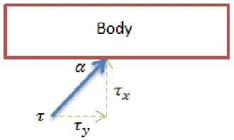
35 Figure 3.3 demonstrates an angular torque and its components that were applied to the
[image:48.612.224.389.141.240.2]chest.
Figure 3.3. Angular Disturbance
The angular torque can be modeled with Equation 3.15, which breaks up the torque into
its components.
(3.15)
Thus, an angular torque can be considered the summation of a sagittal and coronal torque