Numerical simulation of inviscid transient flows in shock tube and its validations

Numerical Simulation of Inviscid Transient Flows

in Shock Tube and its Validations

Al-Falahi Amir, Yusoff M. Z, & Yusaf T

Abstract—The aim of this paper is to develop a new two dimensional time accurate Euler solver for shock tube applications. The solver was developed to study the performance of a newly built short-duration hypersonic test facility at Universiti Tenaga Nasional “UNITEN” in Malaysia. The facility has been designed, built, and commissioned for different values of diaphragm pressure ratios in order to get wide range of Mach number. The developed solver uses second order accurate cell-vertex finite volume spatial discretization and forth order accurate Runge-Kutta temporal integration and it is designed to simulate the flow process for similar driver/driven gases (e.g. air-air as working fluids). The solver is validated against analytical solution and experimental measurements in the high speed flow test facility. Further investigations were made on the flow process inside the shock tube by using the solver. The shock wave motion, reflection and interaction were investigated and their influence on the performance of the shock tube was determined. The results provide very good estimates for both shock speed and shock pressure obtained after diaphragm rupture. Also detailed information on the gasdynamic processes over the full length of the facility is available. The agreements obtained have been reasonable.

Keywords—shock tunnel, shock tube, shock wave, CFD.

I. INTRODUCTION

HIS paper describes the procedure for performance evaluation of a short-duration hypersonic test facility that build at the College of Engineering, Universiti Tenaga Nasional “UNITEN” in Malaysia. The facility is designed so that it can be used as a shock tube, free piston compressor, shock tunnel and gun tunnel. The facility has been designed, constructed and commisioned for a wide range of diaphragm pressure ratios and different driver/driven working gases to get Mach number up to 6. The facility will allow various researches to be done in the field of high speed supersonic and hypersonic flows. The important application would be in power plants where the working fluid is always in a very high speed with high gas effects.

To verify and supplement some of the theoretical results, a hypersonic test facility of a somewhat unconventional design has been built. The bulk of the experimental investigations undertaken to date have dealt with pressure studies using high precision pressure transducers and an in house made fast response thermocouple were used to predict the pressure history and subsequently the shock wave strength P2/P1 and

the surface temperature change profile during the facility operation. Using two pressure transducers the shock wave speed is measured experimentally for different driver/driven gas combinations.

Al-Falahi Amir is with University Tenaga Nasional UNITEN, College of Engineering, Jalan Kajang- Puchong, 43009 Kajang, Selangor Darul Ehsan, Malaysia. e-mail: [email protected]

A two-dimensional time-accurate time-marching Navier-Stokes solver for shock wave applications is described. It uses the second-order accurate cell-vertex finite-volume spatial discretization and fourth order accurate Runge-Kutta temporal integration. Three simulations of particular conditions for a short duration high speed flow test facility are then presented and compared with experimental measurements. The simulations provide very good estimates for both the shock speed and shock strength obtained after diaphragm rapture and also provides detailed information on the gas dynamic processes over the full length of the facility. This detailed information may be used to identify some of the causes for observed variations in pressure and temperature. The agreements obtained have been reasonable.

Construction of this facility is fundamentally important for the development of advanced instrumentation (in this case, fiber optic pressure sensors and fast response thermocouples), and heat transfer/fluid mechanics studies that are relevant to turbine investigations. The wind tunnel provides a convenient and low cost experimental facility that can produce the flow conditions (matched Mach and Reynolds numbers, temperature ratios etc) necessary for experimental simulation of turbulent flows. The advantage of developing instrumentation and investigating relevant flow fields in the wind tunnel environment is derived from the fact that the flow duration is very short (less than 1 second). This is sufficient time to establish the required flow fields and obtain the required measurements, but the energy requirements associated with operating the facility are relatively low. Hence, the facility is a very cost effective way to experimentally investigate critical heat and fluid flow processes associated with turbine power plants.

II. PHYSICAL DESCRIPTION OF THE FACILTY

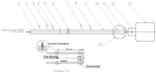
The detail components of the facility are described briefly and shown in Figure 1. This project is a collaboration project between the University of Southern Queensland (USQ) in Australia and Universiti Tenaga Nasional (UNITEN) in Malaysia to design and construct a 10 m short duration hypersonic test facility. The facility consists of the following significant items:

1. Driver section: a high-pressure section (driver), which will contain the high pressure driver gas.

2. Discharge valve: to discharge the driver section after each run.

3. Pressure gauge: to read the pressure inside the driver section, this section is also provided with a static pressure transducer to record the exact value of the driver pressure P4

[image:2.612.46.298.64.181.2]

Fig. 1 schematic diagram of UNITEN’s test facility

4. Vacuum pump: when the driver gas is not air (eg. Helium or Hydrogen) then the driver section should be evacuated and filled with the required driver gas.

5. The primary diaphragm: this is a thin aluminum membrane to isolate the low-pressure test gas from the high-pressure driver gas until the compression process is initiated.

6. Piston compression section: A piston is placed in the barrel (driven tube) adjacent to the primary diaphragm so that when the diaphragm ruptures, the piston is propelled through the driven tube, compressing the gas ahead of it. This piston used with gun tunnel tests only.

7. Discharge valve: to discharge the driven section after each run.

8. Vacuum gauge: to set the pressure inside the barrel section to low values (vacuum values) less than atmospheric value. 9. Barrel section: a shock tube section (smooth bore), to be filled with the required test gas (air, nitrogen or carbon dioxide).

10. Barrel extension: the last half meter of the barrel on which the pressure transducers and thermocouples are to be attached (see details “A”).

11. The secondary diaphragm: it is a light plastic diaphragm to separate the low pressure test gas inside the barrel from the test section and dump tank which are initially at a vacuum prior to the run.

12. Test section: this section will expands the high temperature test gas through a nozzle to the correct high enthalpy conditions needed to simulate hypersonic flow. A range of Mach numbers is available by changing the diameter of the throat insert.

13. Vacuum vessel (dump tank): to be evacuated to about 0.1 mm Hg pressure before running. Prior to a run, the barrel, test section, and dump tank are to be evacuated to a low-pressure value.

It is intended that this CFD solver be a useful tool in the design process of the test facility. The simulation will complement the experimental data. That is any experimental data which could be achieved from the facility need to be verified using a numerical tool.

III. MATHEMATICAL MODEL

In this Section, the fluid flow governing equations are presented in concert with the numerical scheme used to compute the compressible flow within the shock tube.

A. Euler Equation

The two-dimensional continuity, x- and y-momentum and energy equations describing the turbulent flow of a compressible fluid expressed in strong conservation form in the x-, y-Cartesian co-ordinate system may be written as

J y G x F t

w_{+ + =}

∂

∂

∂

∂

∂

∂

(1)

wherewrepresents the conserved variables and

F

and

G

are the overall fluxes in x-, y-directions respectively.

wcan be expressed as:

⎟⎟ ⎟ ⎟ ⎟

⎠ ⎞

⎜⎜ ⎜ ⎜ ⎜

⎝ ⎛

=

0 e v u w

ρ

ρ

ρ

ρ

(2)

F

can be expressed as:

,

0 2

⎟ ⎟ ⎟ ⎟ ⎟

⎠ ⎞

⎜ ⎜ ⎜ ⎜ ⎜

⎝ ⎛

+ =

uh uv

P u

u

F

ρ

ρ

ρ

ρ

(3)

and

G

can be expressed as:

,

0 2

⎟ ⎟ ⎟ ⎟ ⎟

⎠ ⎞

⎜ ⎜ ⎜ ⎜ ⎜

⎝ ⎛

+ =

vh P v uv

v

G

ρ

ρ

ρ

ρ

(4)

e_o and h_o are the specific total internal energy and specific

total enthalpy of the fluid respectively. In the usual notations:

2

2

V

e

e

_o

=

+

₍₅₎

2

2 0

V

h

h

=

+

(6)

2 2

2

=

+

v

u

V

(7)

The body force J is zero vector since effect of gravity is negligible for high speed flow.

⎟⎟ ⎟ ⎟ ⎟

⎠ ⎞

⎜⎜ ⎜ ⎜ ⎜

⎝ ⎛

=

0 0 0 0

J

IV. NUMERICAL SCHEMES

for high speed flow in shock tube. The following sections will discuss the numerical formulation of the modified flow solver.

A. Cell-Vertex Finite-Volume Spatial Discretization The flow domain is replaced by a finite number of control volumes, which are generated algebraically by the current solver. The mesh system is commonly known as H-mesh and divides the physical domain into a set of discrete rectangular control volumes. An example of H-mesh is shown in Figure 2. A cell-vertex formulation is used in which the flow variables are stored at cell vertices A, B, C and D as has been shown in Figure 2. Cell-vertex formulation offers some advantages over the cell-centered one in which cell-vertex method offers higher accuracy on irregular grid.

(i+1, j)

(i+1, j+1)

(i, j+1) (i, j)

Cell (i, j) Boundary S Fixed Area

D C

[image:3.612.333.566.206.360.2]

B A

Fig. 2 An illustration of a typical 2D H-mesh. For a uniform mesh, there would be no difference between the cell-centered and cell-vertex schemes; however, cell-vertex scheme does not require extrapolation to the solid boundary to obtain the wall static pressure, which is necessary in solving the momentum equations for cells adjacent to the solid boundary.

Starting from known values of primitive variables from the previous time-step, the values of

F

and

G

are determined at each node. Then the line integration is performed for each control volume in turn for the four conserved variables.

Integrating Equation (1) with respect to volume

∫

dV

+

∫

(

F

)

dV

+

∫

(

G

)

dV

=

0

t

w

C C

∂

∂

(8)

Using Gauss divergence theorem the whole equation can be reduced to

(

)

∫

−

Ω

−

=

∂

∂

dx

G

dy

F

t

w

C C

1

(9)

Applying the above equation to a typical control volume and defining Ri, j as the residual for the cell, the same discritized

equation for the cell is:

∑

⎟⎟

⎠

⎞

⎜⎜

⎝

⎛

Δ

−

Δ

Ω

−

=

∂

∂

→ →

x

G

y

F

t

w

j i C j i C j i , , , , ,

1

(10)

∑

Ω

=

⎟

⎠

⎞

⎜

⎝

⎛

∂

∂

=

_{C i j}

j i j i j i

R

t

w

w

R

_{, ,}

, ,

,

1

)

(

₍₁₁₎

whereR_ij

( )

w represents the residual for each cell and

)

(

_{, , , ,} , , → →

Δ

−

Δ

−

=

∑

F

y

G

x

R

_{Ci j C i j C i j}

.

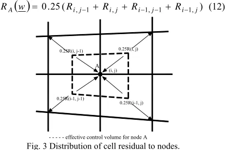
The calculated residuals apply to the values of properties within the cell, whereas, the variables are actually stored at the nodes. Consequently, they have to be redistributed to the four surrounding nodes. This is done by sharing the changes equally between the four nodes as shown in Figure 3, as suggested in the second-order central differencing scheme. Thus:

( )

0.25( _{i,j 1 i,j i 1,j 1 i 1,j})

A w R R R R

R = ₋ + + _{− −} + ₋ (12)

(i, j)

A

- - - effective control volume for node A

0.25R(i-1, j) 0.25R(i-1, j-1)

0.25R(i, j-1) 0.25R(i, j)

Fig. 3 Distribution of cell residual to nodes.

For nodes at the wall, since two cells share a single node, the residual obtained from Equation (12) is doubled. For the nodes at the corners, since only one cell share the node, the residual obtained is quadrupled. Thus, the equivalent discretized equation for node (i, j) will be:

( )

w

R

t

w

A A

=

⎟

⎠

⎞

⎜

⎝

⎛

∂

∂

(13)

B. Treatment of the Inviscid Fluxes

All the inviscid fluxes are calculated by using central differencing scheme, therefore the differencing scheme is second order accurate, from equation (11);

)

(

_{,, ,,} , , → →

Δ

−

Δ

=

∑

F

y

G

x

R

_{Ci j Ci j Ci j}

Applying to control volume shown in Figure 1

) ( ) ( , , , , , , , , , , → → → → → → → → Δ + Δ + Δ + Δ − Δ + Δ + Δ + Δ = x G x G x G x G y F y F y F y F R AD C BA C CB C DC C AD C BA C CB C DC DC C j i C (14) where ) ( 2 1 , ,

,DC C D CC

C F F

F = + ,

) ( 2 1 , ,

,CB C C C B

C F F

) ( 2 1 , ,

,BA C B C A

C F F

F = + ,

) ( 2 1 , ,

,AD C A CD

C F F

F = +

) ( 2 1 , ,

,DC C D C C

C G G

G = + ,

) ( 2 1 , ,

,CB CC CB

C G G

G = +

) ( 2 1 , ,

,BA C B C A

C G G

G = + ,

) ( 2 1 , ,

,AD C A C D

C G G

G = +

C. Artificial Dissipations

All second-order central-differencing schemes, even with a stable time-step, suffer from certain tendencies to instability due to the odd-even decoupling near a discontinuity. The scheme can be stabilized by introducing a small amount of artificial viscosity is suggested by Jameson et al. [11]. This artificial viscosity formulation is a blend of second and fourth-order terms with a pressure switch to detect changes in pressure gradient. The fourth-order terms, for any conserved variables,

w

is:

)

(

)

(

)

(

4 4

4

w

D

w

D

w

D

_ij

=

_xij

+

_yij (15)

where:

]

[

2 1 1 2

4 4

4

6

4

)

(

=

−

xij ij₋

−

ij₋

+

ij

−

ij₊

+

ij₊

xij

w

w

w

w

w

w

D

γ

]

[

i j i j ij i j i j

yij

yij

w

w

w

w

w

w

D

2 1 1 2

4 4

4

6

4

)

(

=

−

γ

−

−

−

+

−

+

+

+

The second-order dissipation terms are defined as:

)

(

)

(

)

(

2 2

2

w

D

w

D

w

D

_ij

=

_xij

+

_yij (16)

where:

]

[

1 1

2 2

2

)

(

=

xij ij−

−

ij

+

ij+

xij

w

w

w

w

D

γ

]

[

i j ij i j

yij

yij

w

w

w

w

D

2

(

)

=

γ

2 ₋₁

−

2

+

₊₁

γ

xij

γ

yij

γ

xij

γ

yij 2

,

2

,

4

and

4

in the above equations are coefficients, which are functions of the local pressure gradient to be defined later.

The fourth-order terms will not affect the global accuracy of the second-order scheme, but they eliminate the background oscillations caused by the central-differencing scheme, which is second-order accurate. However, near a discontinuity, e.g. around a shockwave, they lead to occurrence of oscillations and appearance of overshoots. On the other hand, second-order terms are very dissipative and can eliminate high oscillations near a discontinuity but produce too much background oscillations. Following Jameson et al. [11], the fourth-order terms are turned off near discontinuities, by means of a pressure sensor, and only second-order terms will be in operation in these regions. A

pressure sensor introduced to detect the steepness of the pressure gradient and has the form:

1 1 1 1

2

2

2

− + − +

+

+

+

−

=

ij ij ij ij ij ij xij

P

P

P

P

P

P

X

SF

q

(17)

j i ij j i j i ij j i yij

P

P

P

P

P

P

Y

SF

q

1 1 1 1

2

2

2

− + − +

+

+

+

−

=

(18)

SF2X and SF2Y are second-order dissipation coefficients with

typical values of 0.10-0.50.

The pressure switch defined to turn off the fourth-order and turn on the second-order terms near a discontinuity takes the forms:

γ_xij4 = max (0, SF4X-γ_xij2 ) (19)

γ

yij4 = max (0, SF4Y-γyij

2 _{) (20)}

where:

γ_xij2 = max (q_xij, q_xij+1)

γ

yij2 = max (qyij, qyi+1j)

SF4X and SF4Y are fourth-order dissipation coefficients with

typical values of 0.005-0.01.

It can be seen that near a discontinuity, q and γ 2 are of

order 1 and the second-order becomes the dominant dissipative term. In the remainder of the domain the background dissipation is provided by the fourth-order terms.

SF4X and SF4Y must not be too large since they will create

too much numerical viscosity in the flow domain and thereby mask the physics of the flow.

The total dissipation will be:

( )

w

D

( )

w

D

( )

w

D

ij

=

xij

+

yij (21)

where:

( )

w

D

( )

w

D

( )

w

D

xij xij xij

4 2

−

=

( )

w

D

( )

w

D

( )

w

D

yij yij yij

4 2

−

=

After the addition of the dissipation terms the descritized equation for node A becomes:

( )

w

D

( )

w

R

t

w

A A A

+

=

⎟

⎠

⎞

⎜

⎝

⎛

∂

∂

(22)

The dissipation term

D

_A

( )

w

, is only evaluated in the first stage and frozen for the next three stages of the Runge-Kutta time stepping scheme, as follows.

D. The Multi-stage Runge-Kutta Time Stepping Scheme

Equation (22) is integrated with respect to time by means of a four-stage Runge-Kutta time stepping scheme, as proposed by Jameson et al. [11]:

,

0 n

w

w

=

(

0 0

)

,

1 0 1 D R t w

w = +α Δ +

(

1 0

)

,

2 0 2

D

R

t

w

(

2 0

)

,

3 0 3

D R t w

w = +α Δ +

(

3 0

)

,

4 0 4

D

R

t

w

w

=

+

α

Δ

+

4 1

w

w

n+

=

(23)

where the superscripts, n and n+1 refer to the time intervals in

the main integration sequence, 1, 2, 3, 4 refer to the intermediate time-steps in the Runge-Kutta scheme. The coefficients

α α α α

₁

,

₂

,

₃

,

₄are 0.250, 0.333, 0.500 and 1.000 respectively.

V. BOUNDARY CONDITIONS

A. Solid Boundary

Only the solid boundary condition is considered in the current work since the flow is confined within the tube. At the wall, no-slip boundary condition is imposed for the momentum equations to enforce no mass fluxes can penetrate through the solid boundary. For the energy equation, adiabatic condition is assumed. Solid boundary nodes only have contributions from two cells. However, the control volumes associated with the solid boundary nodes are only half of that for the internal nodes. So, prior to the temporal integration the residuals are doubled.

At the solid boundary, it has been shown by Hirsch [23],

that for Euler equations only one characteristic enters the flow domain and only a single physical boundary condition is to be imposed. This condition is expressed by the vanishing normal velocity:-

Vnormal = 0

As a consequence, all convective flux components through the solid boundary will vanish. This means that in the expression for the flux through a cell face on a solid boundary, only the pressure remains, i.e.:-

F dy G dx P dy

dx

C − C = ₋

⎡

⎣ ⎢ ⎢ ⎢ ⎢

⎤

⎦ ⎥ ⎥ ⎥ ⎥

0

0

(24)

The pressure on the solid boundary face can be calculated directly by taking the average values of the nodes at both ends of the cell face. When the flow is assumed to be inviscid, the velocity at the solid boundary is non-zero.

B. Treatment of Dissipation Terms near the Boundaries

To evaluate the dissipation terms, variables at two neighbouring nodes on either side of the calculating points are required. At the boundary, only variables on one side of the node are known. The other two variables need to be determined by extrapolation. Consistent with Gustafsson and Sundstrom’s [24] recommendations, at the inlet and exit

boundaries, the extra variables are calculated by first-order extrapolation. Only one extra variable is required as the variables at the inlet and exit boundaries are fixed by the inlet and exit boundary conditions respectively. For example, the

extra variable required to calculate the dissipative term at j=

2 is calculated by:-

w

_i0

=

2

w

_i1

−

w

_i2 (25)

It has been observed by Pulliam [25], Swanson and Turkel

[26] and Caughey and Turkel [27] that the treatment of

dissipation terms, especially at the solid boundaries, can have a strong effect on the accuracy and convergence rate of a viscous or even inviscid flow computation. An important conclusion that can be drawn from these studies is the necessity to reduce the second-order dissipation terms at the solid boundaries. The treatment used is that recommended by

Pulliam [25] and used by Bamkole [28] and Zamri [21,22].

Modifications are only needed for the pitchwise components,

D

yij

( )

w

. At i = 1, the fourth-order components

are replaced by the second-order one by using one-sided difference, while the second-order terms are set to zero. So,

[

]

D

y j1

w

y j

w

j

w

j

w

j 4

1 4

1

2

2 3

(

)

= −

γ

−

+

(26)

At i = 2, the extra variable needed for the fourth-order

terms is calculated by means of a first-order extrapolation. With reference to Figure (2), the resultant term will become: -

]

[

D_{y j}2 w _{y j} w j w j w j w j

4

2 4

1 2 3 4

2 5 4

( )= −

γ

− + − + (27)

VI. INITIAL CONDITIONS

To start the iterations, initial flow field variables must be specified at all calculating points. In the current work, the pressure values are specified at both the driver and driven sections, in accordance with the desired pressure ratio. The flow is assumed to be in stagnant condition initially.

VII. STABILITY CRITERIA

Generally, explicit time-marching schemes suffer from instability problem, particularly when the time step is larger than that from the Courant Friedrichs Lewy (CFL) criterion. In order to ensure numerical stability, the maximum allowable time-step which can be used in the calculation is limited by:

(

V a

)

x CFL t

+ Δ ≤

Δ . (28)

where

CFL = CFL number,

Δx = incremental distance,

V

= speed,

a = speed of sound =(γRT)0.5 .

For the four-stage Runge-Kutta scheme applied in a 1D problem to be specific, CFL =

2 2

. However, this number

VIII SOLUTION PROCEDURE

The solution procedure of the solver can be summarized as follows:-

Step 1: Generate the structured H-mesh. The details of the mesh system will be explained in the following sections.

Step 2: Initialise the flow variables at time = 0s.

Step 3: Initiate the 4-stage Runge-Kutta (RK) time integration scheme. Here, the spatial integration of the governing equations to determine the residual in Equation 11 is calculated for the first RK stage. The cell residuals are then redistributed back to the neighbouring vertices using Equation 12. The solution vector is then time marched (see Equation 23) using the residuals for each vertex and the corresponding stage coefficient (α).The flow variables are then updated accordingly. Step 4: Step 3 is repeated until the maximum Runge-Kutta

stage (in this case is 4) is reached.

Step 5: Save the pressure value at the first station (refer to Figure 4). Update the time level (tn+1=tn+Δt). Go to

[image:6.612.361.511.339.728.2]

Step 3 until the desired time level is reached.

Fig. 4 Location of station 1 and 2

IX. VALIDATION OF THE CFD CODE

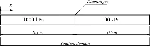
To ensure the validity of the CFD code, in terms of the ability to capture shocks and contact discontinuity and to produce the correct pressure, density and speed profiles, the code has been validated against anexact solution for Inviscid Flow in Shock Tube.The situation considered is basically that in a shock tube with a pressure difference applied across the diaphragm. The initial conditions are shown in Figure 5.

100 kPa 1000 kPa

0.5 m 0.5 m

Solution domain Diaphragm

[image:6.612.56.298.520.594.2]

x

Fig. 5 Solution domain

The direction x is chosen in the direction shown in Figure

6 because the air flow that develops after the diaphragm ruptures will be from the high pressure section towards the low pressure section, i.e. x is chosen to be in the direction of

the induced flow.

The Sod problem [29] is an essentially one-dimensional flow discontinuity problem which provides a good test of a compressible code's ability to capture shocks and contact discontinuities with a small number of zones and to produce the correct density profile in a rarefaction.

The problem spatial domain is 0 ≤ x ≤ 1. The initial

solution of the problem consists of two uniform states, termed as left and right states, separated by a discontinuity at the origin, xo = 0.5. The fluid is initially at rest on either side of

the interface, and the density and pressure jumps are chosen so that all three types of flow discontinuity (shock, contact, and rarefaction) develop. To the ``left'' and ``right'' of the interface we have,

ρL = 1 ρR = 0.125

PL = 1 PR = 0.1

uL = 0 uR = 0

The ratio of specific heats γ is chosen to be 1.4 on both sides of the interface.

A uniform grid spacing with the number N = 356 is used. The boundary conditions of the problem are held fixed as a short time span of the unsteady flow is considered. The wave pattern of this problem consists of a rightward moving shock wave, a leftward moving rarefaction wave and a contact discontinuity separating the shock and rarefaction waves and moving right rightward. Figure 6 shows comparisons between the present results for the pressure, density and Mach number at a time t = 0.2 ms and the exact solutions. It can be observed

that the present work is capable of capturing the different types of discontinuities quite accurately.

Distance (m)

Pr

es

su

re

(P

a)

0 0.25 0.5 0.75 1 1.0E+05

2.0E+05 3.0E+05 4.0E+05 5.0E+05 6.0E+05 7.0E+05 8.0E+05 9.0E+05 1.0E+06

Exact CFD P4= 1000 kPa P1= 100 kPa N=356

Distance (m)

Density

(kg/m

3)

0 0.25 0.5 0.75 1 1

2 3 4 5 6 7 8 9 10 11 12

Exact CFD

P4 = 1000 kPa P1 = 100 kPa N = 356

Shock wave Contac surface

Distance (m)

Mac

h

0 0.25 0.5 0.75 1 0

0.1 0.2 0.3 0.4 0.5 0.6 0.7 0.8 0.9 1

Exact CFD

P4= 1000 Pa P1= 100 kPa N=356

Fig. 6 Results for the Sod’s shock tube problem at t = 0.2

The mesh size plays important role in determining the accuracy of the numerical solution. In order to understand this role the mesh size in x-direction has been investigated. Three different cases with different mesh size (N = 256, N = 356, and N = 456) and a diaphragm pressure ratio P4/P1 =10 have

been used. Figure 7 shows the effect of using larger number of grid points in x-direction and how the solution is affected accordingly. From the Figure 8 it will be seen that the details of the shock wave are well captured when a larger number of grid points are used and the program becomes more stable and less oscillation is produced. Also the numerical and exact solutions are now very comparable when number of grid points N = 456 is used. Consequently, N = 456 have been used in all of the following runs.

Distance (m)

Pressure

(Pa)

0 0.25 0.5 0.75 1 1.0E+05

2.0E+05 3.0E+05 4.0E+05 5.0E+05 6.0E+05 7.0E+05 8.0E+05 9.0E+05 1.0E+06

Exact CFD

P4= 1000 kPa P1= 100 kPa N= 256

High oscillation

Distance (m)

P

ressu

re

(Pa

)

0 0.25 0.5 0.75 1 1.0E+05

2.0E+05 3.0E+05 4.0E+05 5.0E+05 6.0E+05 7.0E+05 8.0E+05 9.0E+05 1.0E+06

Exact CFD P4= 1000 kPa P1= 100 kPa N=356

Less oscillation

Distance (m)

Pr

ess

ur

e

(

Pa

)

0 0.25 0.5 0.75 1 1.0E+05

2.0E+05 3.0E+05 4.0E+05 5.0E+05 6.0E+05 7.0E+05 8.0E+05 9.0E+05 1.0E+06

Exact CFD P4=1000 kPa P1=100 kPa N=456

Good stability

Fig. 7 Pressure History at Different Mesh size in X-Direction at t =

0.2 ms

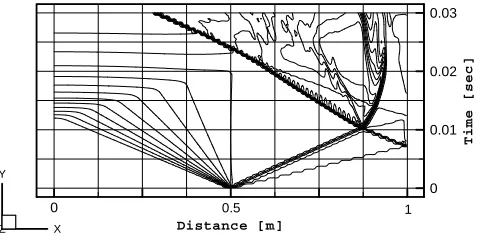
The x-t diagram is one of the important tools which

give a good estimation for the maximum useful test time that can be obtained after removal of the diaphragm. Figures 8 and 9 show the predicted x-t diagram for pressure and density profiles obtained for an air-air gas combination run. The diaphragm pressure ratio used for this simulation is (P4/P1)

=10. Figure 8 represents the x-t diagram for the pressure

history; the contact surface does not appear in this figure as it follows the shock wave continuously as it apparent in Figure

6, however it is very clear in Figure 9 which shows the x-t history for the density profile.

0 0.01 0.02 0.03

Ti

me

[se

c]

0

Distance [m]

X Y

Z

[image:7.612.319.557.81.198.2]

0.5 1

[image:7.612.93.255.221.620.2]

Fig. 8 x-t diagram for pressure history

Figure 9 represents the density history along the whole length of the test facility. Both of the shock wave and the contact surface are displayed in this figure. The shock wave is followed by the contact surface until the reflected shock wave interact with the contact surface and then the wave is further reflects. The expansion waves are displayed in the two figures and due to the sufficient length of the driver section the shock wave and contact surface are intersected before the reflected expansion waves reach the end of the driven section.

0 0.01 0.02 0.03

Time

[sec]

0

Distance [m]

X Y

Z

0.5 1

Fig. 9 x-t diagram for density history

X. INVISCID TRANSIENT FLOW IN SHOCK TUBE

In this study, a sensitivity study on the flow model used has been performed as well as the time-step size, towards the accuracy of the flow solution applied for a shot with similar gases allocated in both the driver and driven sections (air-air). CFD solution for inviscid simulation for a diaphragm pressure ratio P4/P1 of 10 will be discussed. The simulation has been

conducted using the actual dimensions of the test facility shown in Figure 10.

[image:7.612.317.557.343.467.2]

[image:8.612.364.512.50.176.2]

Fig. 10 Mesh spacing allocated for each section

The pressure, temperature, density and Mach number of the flow were stored in two stations, the first station is at the x

= 6183 mm from the left hand side end of the driver section, the second station is with an axial separation of 342 mm from the first station as shown in Figure 11.

Station 2 Station 1

wall end Flow direction

Barrel

[image:8.612.48.302.51.95.2]

40 342

Fig. 11 The two stations at the end of shock tube

The pressure history for the above mentioned shot is depicted in Figure 12 from which one can follow the physics of the flow inside the shock tube. The first jump represents the shock wave, for which the pressure inside the barrel increases from 100 kPa to around 220 kPa. As the shock wave proceeds to the end of the tube it will hits the wall and reflects moving in the opposite direction increasing the pressure to about 450 kPa. The shock wave will then interact with the contact surface which is following the shock wave, and due to this interaction between the shock wave and the contact surface the pressure will be increased until it reaches its peak pressure value of 530 kPa.

.

Time [sec]

P

res

su

re

[P

a

]

0 0.005 0.01 0.015 0.02 0.025 1.0E+05

1.5E+05 2.0E+05 2.5E+05 3.0E+05 3.5E+05 4.0E+05 4.5E+05 5.0E+05 5.5E+05

Station 1 Station 2

[image:8.612.60.278.171.266.2]

Shock wave Reflected shock wave

Fig. 12 Pressure history for inviscid flow (air-air, P4/P1=10)

The shock wave speed can be determined from the CFD data obtained from this simulation. As the distance between the two stations is known (0.342 m) and the time of shock travels from station 1 to station 2 can be obtained from the pressure history graph, as show in Figure 13, the shock wave speed is determined for this shot is 518 m/s. comparing to the theoretical value for this pressure ratio (550 m/s) the percentage error is around 6% which is reasonable

Time [sec]

P

ressur

e

[Pa

]

0.0066 0.0068 0.007 0.0072 0.0074 1.0E+05

1.5E+05 2.0E+05

Station 1 Station 2

t = 0.0066 sec

[image:8.612.365.512.330.457.2]

Δ

Fig. 13 Shock wave speed (inviscid flow)

Using the same procedure, the reflected shock wave speed can be determined as the wave reflects from the tube end and moves in the opposite direction (left direction), due to impact with the end wall the wave will lose some of its kinetic energy and consequently its speed decreases to about 342 m/s, as shown in Figure 14 which represents a close view for the reflection region in the pressure history graph. The time period from station 2 to station when is around 0.001 sec which is longer than the time period when the shock travels from station 1 to station 2 due to the energy lost after reflection.

Time [sec]

Press

ure

[

Pa]

0.0075 0.008 0.0085 2.5E+05

3.0E+05 3.5E+05 4.0E+05 4.5E+05

Station 1 Station 2

t = 0.001 sec

Δ

Fig. 14 Reflected sock wave speed

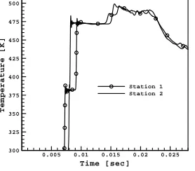
The same trend can be noted when the temperature history is investigated as shown in Figure 15. The first jump in the temperature profile represents the shock wave and the second jump is due to the reflected shock wave. The temperature is increased from the initial value 300 K to about 380 K due to shock wave affect and when the shock reflects from the tube end the temperature rises to 475 and after interaction between reflected shock wave and the contact surface the flow temperature becomes about 490 K.

Time [sec]

Te

mp

er

atu

re

[

K]

0.005 0.01 0.015 0.02 0.025 300

325 350 375 400 425 450 475 500

Station 1 Station 2

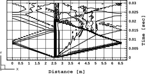
[image:8.612.95.246.445.576.2] [image:8.612.372.511.584.706.2]

The x-t diagram is one of the important tools which give a good estimation for the maximum useful test time that can be obtained after removal of the diaphragm. Figures 16 and 17 show the predicted x-t diagram for pressure and density profiles obtained for an air-air gas combination run. The diaphragm pressure ratio used for this simulation is (P4/P1) =10.

0 0.005 0.01 0.015 0.02 0.025 0.03

Ti

m

e

[

se

c]

0 0.5 1 1.5 2 2.5 3 3.5 4 4.5 5 5.5 6 6.5

Distance [m]

X Y

[image:9.612.317.569.52.187.2]

Z

Fig. 17 x-t diagram for the pressure profile (inviscid flow)

Figure 18 represents the density history along the whole length of the test facility. Both of the shock wave and the contact surface are displayed in this figure. The shock wave is followed by the contact surface until the reflected shock wave interact with the contact surface and then the wave is further reflects. The expansion waves are displayed in the two figures and due to the sufficient length of the driver section the shock wave and contact surface are intersected before the reflected expansion waves reach the end of the driven section.

0 0.005 0.01 0.015 0.02 0.025 0.03

Tim

e

[

sec]

0 0.5 1 1.5 2 2.5 3 3.5 4 4.5 5 5.5 6 6.5

Distance [m]

X Y

[image:9.612.53.294.144.266.2]

Z

Fig. 18 x-t diagram for the density profile (inviscid flow)

Finally, to investigate the flow properties in 2D scheme, the results of the numerical simulations have been displayed in contour plots. The contour plot of the pressure history along the facility is shown in Figure 19. Time step used in this simulation is 0.000005 sec and the total number of iterations is 6000. The solver is programmed so that it stores the output data after each one hundred iterations, subsequently there will be 60 output files. Each file represents the data after 0.0005 sec. As shown in this Figure, driver pressure P4=100 kPa and

pressure in the driven section P1 is 10 kPa.

Fig. 19 Contour plot for pressure history at t = 0

[image:9.612.317.563.250.321.2]

After diaphragm rupture, shock wave travels right through the barrel while the expansion wave travels left through the driver section. These two waves are captured after 0.005 sec and shown in Figure 20.

Fig. 20 Shock and expansion waves

[image:9.612.316.567.396.459.2]

These two waves continue their journey towards the tube ends, at time 0.0081 s the shock wave hits the barrel end on the right hand side while the expansion wave reaches the left hand side of the facility as shown in Figure 21.

Fig. 21Shock and expansion waves at the facility ends

[image:9.612.50.292.410.529.2]

The two waves then will reflect from the end of the tube as shown in Figure 23.

Fig. 22 Shock and Expansion wave reflection

[image:9.612.317.567.511.580.2]

The reflected shock wave now moves to the left towards the contact surface while the reflected expansion wave moves to the right towards the contact surface and shock wave as shown in Figure 23.

[image:9.612.319.561.654.713.2]

[image:10.612.65.281.109.250.2]

The shock wave interacts with the discontinuity surface and reflects again. This process continues for several times until getting pressure balance along the whole facility as shown in Figure 24.

Fig. 24 Interaction between shock wave and contact surface

Figure 25 shows velocity contour at t= 0.0029 sec after diaphragm rapture, at this ime the shock did not reflects yet, consequently the flow is symmetry and uniform in y-direction.

Fig. 25 Velocity contour before shock reflection

[image:10.612.50.293.442.473.2]

As the shock wave reflects from the tube end it will move to the left and interact with the discontinuity surface and the flow no longer symmetry as shown in Figure 26.

Fig. 26 Velocity contour after shock reflection

XI. CONCLUSIONS

The paper described the formulation of the 2D-CFD solver designed for simulation of flow in shock tube. The program has been applied to a standard case of inviscid flow in shock tube. The agreement with the analyzed solution is very good which proved the validity of the basic numerical scheme developed.

The present code showed good capability to provide the x-t diagram successfully. From this diagram one can determine the useful duration (for this case it is about 10 ms), which is quite comparable compared to other facilities. It can be concluded, based on the agreement with the analytical results, that the numerical formulation for the inviscid part of the solver is valid.

The results presented in this paper show that two-dimensional modeling of the hypersonic test facility is an effective way to obtain facility performance data. Although this paper focused on the HTF facility, the CFD code is generic and may be applied to other facilities.

The code could be further improved if a cylindrical coordinate system is used for mesh generation instead of the Cartesian coordinate system currently used. The simulations had successfully indicated that the flow is symmetry before shock wave reflection off the tube end and the flow is disturbed after shock reflection and interaction with contact discontinuity.

REFERENCES

[1] Caleffi, V., Valiani, A. and Zanni, A. (2003), ‘Finite Volume Method for Simulating Extreme Flood Events in Natural Channels’, Journal of Hydraulic Research, Vol. 41, No. 2, pp. 167-177.

[2] Valiani, A., Caleffi, V. and Zanni, A. (2002), ‘Case Study: Malpasset Dam-Break Simulation using a 2D Finite Volume Method’, Journal of Hydraulics Engineering, Vol. 128, No. 5, pp. 460-472.

[3] McDonald, P.W. [1971] 'The Computation of Transonic Flow Through 2D Gas Turbine Cascades’ ASME Paper No. 71-GT-89 [4] Couston, M. [1976] 'Time-Marching Finite Area Method' V.K.I.

Lecture Series 84

[5] Thiaville, J.M. [1977] 'Comparison of a Finite Difference Method with a Time-Marching Method for Blade to Blade Transonic Flow Calculations' . in ‘Transonic Flow Problems in Turbomachinery’, (ed.

Adamson, T.C & Platser, M.F.)

[6] Farn, C.L. and Whirlow, D.K. [1977] 'Application of Time-Dependent Finite Volume to Transonic Flow in Large Turbine' in ‘Transonic Flow Problems in Turbomachinery’, (ed. Adamson, T.C & Platser, M.F.)

[7] Denton, J.D. [1975] 'A Time Marching Method for Two- and Three-Dimensional Blade to Blade Flows' ARC R. & M. No. 3775

[8] Lerat, A. and Sides, J. [1982] 'A New Finite Volume Method for the Euler Equations with Applications to Transonic Flows' in ‘Numerical Methods in Aeronautical Fluid Dynamics’, (Ed. Roe, P.L), Academic Press, pp. 245-288

[9] Rizzi, A. and Eriksson, L.E. [1981] ‘Transfinite Mesh Generation and Damped Euler Equations Algorithm for Transonic Flow Around Wing-Body Configurations’ . AIAA 5th Computational Fluid Dynamics Conference, Paulo Alto, pp. 43-68

[10] Rizzi, A. [1982] ‘Damped Euler-Equations Method to Compute Transonic Flow Around Wing-Body Combinations’ AIAA Journal, Vol. 20

[11] Jameson, A., Schmidt, W. and Turkel, E. [1981] 'Numerical Solutions of the Euler Equations by Finite Volume Methods using Runge-Kutta Time Stepping Schemes' AIAA Paper No. 81-1259

[12] Jameson, A. [1982] 'Transonic Aerofoil Calculations Using the Euler Equations' Numerical Methods in Aeronautical Fluid Dynamics (P.L. Roe ed.), Academic Press, pp. 289-308

[13] Jameson, A. and Baker, T.J. [1983] 'Solution of the Euler Equations for Complex Configurations' Proc. of the AIAA 6th Computational

Fluid Dynamics Conference, AIAA, New York, pp. 293-302 [14] Buratynski, E.K. and Caughey, D.A. [1986] 'An Implicit LU scheme

for the Euler Equations Applied to Arbitrary Cascades' AIAA Journal, 24 (1): 39-46

[15] Dawes, W.N. [1987] 'Application of a Three-Dimensional Viscous Compressible Flow Solver to a High-Speed Centrifugal Compressor Rotor - Secondary Flow and Loss Generation' Proc. Inst. Mech. Engrs., Conf. Turbomachinery Efficiency, Prediction and Improvement, C261-87, pp. 53-61

[16] Van Leer, B. [1979] ‘Towards the Ultimate Conservative Difference Schemes. V. A Second Order Sequel to Gudunov’s Method’ J. Comp. Physics, 32 : 101-36

[17] Harten, A. [1983] ‘High Resolution Schemes for Hyperbolic Conservation Laws’ Journal of Computational Physics, 49, 357-93

[18] Harten, A. [1984] ‘On a Class of High Resolution Total Variation Stable Finite Difference Schemes’ SIAM Journal of Numerical Analysis, 21, 1-23

[19] Osher, S. [1984] ‘Riemann Solvers, the Entropy Condition and Difference Approximation’ SIAM Journal Numerical Analysis, 21, pp.

217-35

[21] Yusoff M. Z. [1997]‘ An improved treatment of two-dimensional Two-Phase Flow of Steam by a Runge-Kutta Method’,Ph.D. Thesis, University of Birmingham

[22] Yusoff M. Z. “A Two-Dimensional Time-Accurate Euler Solver for Turbo machinery Applications” Journal-Institution of Engineers, Malaysia Vol. 5 No. 3 1998

[23] Hirsch, C. [1990] ‘Numerical Computation of Internal and External Flows’

Volume 1(Fundamentals of Numerical Discretization) and Volume 2 (Computational Methods for Inviscid and Viscous Flows), John Wiley & Sons

[24] Gustafsson, B. and Sundstrom, A. [1978] ‘Incompletely Parabolic Problem in Fluid Dynamics’ SIAM Journal of Applied Mathematics,

35 (2): 343-357

[25] Pulliam, T.H. [1986] ‘Artificial Dissipation Model for the Euler Equations.’ AIAA Journal , 24: 1931-1940

[26] Swanson, R.C. and Turkel, E. [1987] ‘Artificial Dissipation and Central Difference Schemes for the Euler and Navier Stokes Equation.’ AIAA Paper No. 87-1101, Proc. AIAA 8th Computational

Fluid Dynamics Conference, pp. 55-69

[27] Caughey, D.A. and Turkel, E. [1988] ‘Effects of Numerical Dissipation of Finite Volume Solutions of Compressible Flow Problems’ AIAA Paper No. 88-0621, AIAA 26th Aerospace Sciences

Meeting

[28] Bamkole, B.O. [1991] ‘A Two Step Method for Solving the Euler Equations’ Internal Report, Manuf. & Mech. Eng. Dept., University of Birmingham

[29] G. A. Sod, A survey of several finite difference methods for systems of nonlinear hyperbolic conservation laws, J. Comput. Phys. 43 (1978)

1-31

NOMENCLATURE

a Speed of sound

D Artificial dissipation component

e Specific internal energy

eo Total internal energy

F

Axial component of the inviscid flux vector

FT Time step factor

G

Tangential component of the inviscid flux

vector

ho Stagnation enthalpy

h Specific enthalpy

P Static pressure

Po Stagnation pressure

Pb Downstream static pressure

R Flux residual

SF2X Second order smoothing factor in axial

direction

SF2Y Second order smoothing factor intangential

direction

SF4X Fourth order smoothing factor in axial

direction

SF24Y Fourth order smoothing factor intangential

direction

T Temperature

t Time

Δt Time step for main calculation

V Overall velocity

Vx Velocity component in axial direction

Vy Velocity component in tangential direction

w

Conserved variable vector

x Axial distance

y Tangential distance

Greek Symbols

α Integration constant in Runge-Kutta time

stepping

β Enthalpy damping coefficient or coefficient

in scaling factor equation

ε Pressure gradient sensor

ρ Density

θ Implicit residual averaging coefficient

Ω Volume of element

γ Artificial dissipation coefficient component

Subscript

o Stagnation condition

x Cartesian co-ordinates

y Cartesian co-ordinates

1 Initial state in driven section

2 Flow conditions between shock wave and

contact surface

3 Flow conditions between rarefaction wave

and contact surface