Scarmana, G. (2009). Limits of Multi-frame Image Enhancement: A Case of Super-resolution. In: Ostendorf B., Baldock, P., Bruce, D., Burdett, M. and P. Corcoran (eds.), Proceedings of the Surveying & Spatial Sciences Institute Biennial International Conference, Adelaide 2009, Surveying & Spatial Sciences Institute, pp. 577-587. ISBN: 978-0-9581366-8-6.
LIMITS OF MULTI-FRAME IMAGE ENHANCEMENT: A CASE OF
SUPER-RESOLUTION
Gabriel Scarmana
Department of Main Roads, Queensland, Australia Email address
ABSTRACT
A common and important problem that arises in visual communications is the need to create an enhanced-resolution video image sequence from a lower resolution input video stream. This can be accomplished by exploiting the spatial correlations that exist between successive video frames using Super-Resolution (SR) reconstruction. SR refers to the task of increasing the spatial resolution through multiple frame processing.
Multi-frame resolution enhancement methods are of increasing interest in digital image processing and there has been a substantial amount of research in developing algorithms that combine a set of low-quality images to produce a set of higher quality images. Either explicitly or implicitly, such algorithms must perform the common task of registering and fusing the low-quality image data. While many such processes have been proposed, very little work has addressed their limits.
In this context, an algorithm designed to operate in the spatial domain is used in a controlled test to compute a higher-resolution image by mapping a model of the image formation process using local sub-pixel shifts among the lower resolution and compressed images of the same scene. These shifts are determined by way of a rigorous least-squares area-based image-matching scheme that does not require control points.
Statistical results show that the performance of the algorithm does degrade, as would be expected, depending on (1) the amount of noise present in the low-resolution images, (2) the number of low-resolution input images and (3) the magnification factor required to meet resolution requirements.
INTRODUCTION
SR is a term given to a single image product that has been produced by combining a number of images of the same scene, using algorithms that increase spatial resolution. Subtle sub-pixel shifts in each image will, when combined, allow for a composite image to be sampled at more points than provided by the sensor’s detector array. The composite image will also have a sharper point spread. SR finds applications in the following field of expertise:
578
geometric distortion that may exist among the low-resolution images is more uniform within a small region.
Security/Forensics: where a typical single frame of a video signal is generally poor for hard copy printouts. Enhancement of a freeze image can be done by using several successive images merged together by SR. This may be helpful during judicial enquiries where video recordings are used as evidence to identify suspects. In fact, faces often appear very small in surveillance imagery because of the wide fields of view that are typically used and the relatively large distance between the cameras and the scene. For tasks such as face recognition, resolution enhancement techniques are often needed.
Defence: images taken from satellites or drones may be very expensive, because of the cost of infrared cameras, and constraints over weight and volume. Improving quality is essential to optimise these images. Reconstruction-based SR is utilised for recognising and tracking targets in real time for weapons guidance systems or for improving reconnaissance photo-interpretation of satellite imagery when seeking sensitive targets.
Medical and scientific: CT, MRI and ultrasound are common applications. Other examples may include imaging used in microscopy or astronomy. Automatic vision techniques used with robotic assembling, or detection of defective pieces can also take advantage of SR.
The author acknowledges the rapid advances which have been made in hardware solutions for image sensors to solve the problem of increasing the resolution of digital images. The work presented here does not detract from those advances; rather it provides a complementary algorithmic technique which is hardware independent. This algorithm can increase the resolution of any image sequence taken from any digital imaging capturing device.
The spatial resolution of the super-resolved image is user-selectable as a grid ratio (p), that is, the object-space length of one (input) low-resolution pixel as related to the length occupied by a desired (output) high-resolution pixel. For example, a grid ratio p = 3.0 means that each of the high-resolution pixels of the enhanced composite is 3.0 times smaller, in each linear direction, than any low-resolution pixel of the input images.
The theoretical limit for the grid ratio is dictated by sampling theory which guarantees the accurate reconstruction of a signal. In this case, each row of the digital image is considered to represent an ‘‘image signal’’. The sampling theorem means that to mathematically represent fully the spatial details of an original continuous-tone image, the image must be sampled at a rate of at least twice that of the highest spatial frequency contained in it.
To capture an image’s finest dark-to-light-to-dark detail, sampling must occur so that at least two samples (two low-resolution pixels) fall in these detail sections (high-resolution pixels). This ensures that both the dark and light portions of the detail are sampled, and hence preserved, in the resulting digital image. The Nyquist frequency is the term referred to this sampling rate (Gonzalez and Woods, 2007).
However, the achievable improvement in resolution which is possible using SR techniques may have certain limitations different to the above theoretical definitions. For instance, if the grid ratio becomes too large and noise is added to the low-resolution images or the registration process is inaccurate, the performance of SR algorithms deteriorates. The images they produce are either overly smooth or contain undesirable details. Exploring the limits of SR to discover such limits is important, so that practitioners may use appropriate magnification factors, thus saving resources.
579
divide the original image into blocks which are processed independently. At high compression ratios, the boundaries between the blocks become visible and lead to ‘‘blocking’’ artefacts (Russ, 2007). If these coding effects are not removed, SR techniques may produce a poor estimate of the resolution sequence, as coding artefacts may still appear in the high-resolution composite (Tom and Katsaggelos, 2001).
A number of algorithms for the enhancement of resolution in images of static objects have appeared in the literature (Farsiu et al., 2004; Fryer and McIntosh 2001; Scarmana and Fryer, 2006; Hendricks and van Vliet., 1999; Zhouchen et al., 2004; Vandewalle et al. 2005). The majority of this literature on algorithmic SR describes the use of three basic steps: (1) estimation of the motion fields or shifts among the different low-resolution images at a sub-pixel level (sometimes referred to as image-to-image registration or image matching); (2) projecting or mapping the pixels of the low-resolution images onto a higher resolution grid using the motion fields detected and; (3) interpolating or solving sets of equations derived from the geometric relationships existing between low and high-resolution pixels.
While these three steps are crucial for obtaining a higher resolution composite, discussion on their limitations is rare and incomplete. Hence, this paper attempts to explore these limitations using a case study aimed to define the required number of low-resolution images in the presence of compression artefacts, added noise and/or the occurrence of potential misregistrations. Theoretical aspects of the proposed image enhanced process are discussed in the ensuing sections.
SUB-PIXEL MOTION ESTIMATION
The sub-pixel registration between two images of the same scene is derived from image registration or matching (Wolf and Dewitt, 2000). The image registration technique used in this work matches the intensity values of two digital images, while simultaneously detecting, and locating, any geometric differences that exist between the two images. These geometric differences relate to potential shifts and rotations between the frames being investigated.
This method is known as a least squares area based matching technique and can overcome difficulties arising from radiometric differences in the images being matched to achieve sub-pixel accuracies of approximately 0.1 sub-pixels. The reader is referred to see Pilgrim (1991) for the theory and formulations behind this process. Three basic assumptions are made: (1) The initial match position and orientation are not known before the registration process begins; (2) the magnitude and extent of the differences that exist between the images, if any, are assumed to be unknown; and (3) the technique is not an approximate registration procedure, but an accurate one.
The technique allows images to be registered without using control points in the registration procedure. For a correct detection of the shifts or offsets between two images, the images must contain some features that make it possible to match two undersampled images. Very sharp edges and small details are most affected by aliasing, so they are not reliable to be used to estimate these shifts. Uniform areas are useless, since they are translation invariant. The best features are slow transitions between two areas of grey values.
These areas are generally unaffected by aliasing and such portions of an image need not to be detected specifically, although their presence is very important for an accurate registration result. Hence, prior to registering two or more images of the same scene it is recommended to remove details affected by aliasing by applying a low-pass filter to the images. The purpose of a low-pass filter is to “smooth” sharp edges, small details, sudden changes of intensity values and distortions created by compression processes (Vandewalle et al., 2005).
580
sequence of images. By calculating these shifts with respect to a single reference image, only one realization of the relative positions is obtained. By repeating the procedure for another reference image, a second estimate for the relative positions is made. Continuing to repeat this process for all images in the sequence, a better estimate of the relative shifts, image to image, can be found.
The statistical measure used to determine the “best” possible value for all such possible combinations of the motion vectors between two given low-resolution images was the vector median. The implementation of the vector median was considered more appropriate than, for instance, the vector mean. If the vector mean was taken instead of the median, then the final motion vector would be an entirely new vector, and not one of the vectors originally estimated. In addition, the mean is less robust than the median if outliers are present (Spiegel, 1999).
MAPPING THE LOW-RESOLUTION IMAGES
Each pixel within a scale image, shown in Figure 1 as a square area, contains a single grey-scale value representing the average intensity value, of all the details in the area it covers. The grey-scale value of each pixel is usually an eight-digit binary number representing a shade of grey from total black to total white in 256 gradations. The human eye can detect only about 32 different levels of grey, so the digital imaging and subsequent processing constitutes at least a four-fold improvement over visual processes (Russ, 2007).
In Figure 1(a), the observed data represents a portion of one single line that a camera/scanner records as it passes over the object. As the diagram shows, an averaging of values occurs where the edges of the darker object fall within the area of the camera’s pixel definition. In Figure 1(a) the camera records a value of 200 instead of either 250 or 166. In the recorded “low-resolution” data the sharp edges of the object are “lost” and the object may be unrecognisable.
However, the relationships between the values of the pixels contain more information about the original shape of the object than is visible to the eye. Because the specific variation of pixel values was originally derived from averaging of the values in the actual scene, with appropriate algorithms the original shape of the object can often be recovered. Such a procedure involves the original pixel and the values of immediately surrounding pixels.
(a) (b)
Fig. 1: (a) Pixel integration of edge areas and (b) Two low-resolution pixels (C1 and C2) mapped on the higher resolution grid (X1, X2….X15, grid ratio p= 2.0).
X1 X2 X3 X4 X5
X7 X8 X9 X10
X11 X12 X13 X14 X15
C1 C2
250 166 166 250
Physical Landform Sensor track
Recorded data
Pixel value returned after averaging for the scanned area
200 166 166 200 250
250
[image:4.595.107.515.482.665.2]581
In the proposed technique each pixel of the low-resolution images is examined one by one and mapped onto a higher resolution grid. For instance, in Figure 1(b), the proportion of high-resolution pixels that contributed to the formation of the low-high-resolution pixels C1 and C2 can be estimated in terms of grey scale values using an algebraic approach based on a weighted geometric mean of values (Spiegel and Stephens, 1999).
The geometric mean uses logarithmic expressions to evaluate data covering several orders of magnitude, for estimating ratios and percentages, or other data sets bounded by zero. Also, the intensity response of the eye is logarithmic and therefore it may sometimes be preferable to quantise and process images on a logarithmic scale rather than a linear scale. From Figure 1(b) each of the low-resolution pixels (C1 and C2) can be expressed in terms of a weighted geometric mean as shown in Equation 1 below.
Log Ci = ( ai log Xi) * N-1 (1)
In this equation C is the low-resolution input pixel. The term ai represents the partial areas of
high-resolution pixels (Xi) affected by each low-resolution pixel. All the Xi are positive
numbers. N is the summation of all the ai which in the case of Figure 1(b) is equal to 4. Note
that N=p2 being p the grid ratio which determines the dimensions of the image in high-resolution pixels with respect to the dimensions of the image in low-high-resolution pixels. Upon applying equation (1) to the cases of C1 and C2 in Figure 1(b) the following two equations can be constructed:
logC1 = (0.25logX1+0.5logX2+0.25logX3+0.5logX6+logX7+0.5logX8+ 0.25logX11+0.5logX12+0.25logX13)/4. (2)
logC2 = (0.25logX3+0.5logX4+0.25logX5+0.5logX8+logX9+0.5logX10+ 0.25logX13+0.5logX14+0.25logX15)/ 4. (3)
The resolution pixel coordinate system defines the position of all the unknown high-resolution pixels and is the system onto which the low-high-resolution images are mapped. Once the first low-resolution pixel (C1) is related to the high-resolution coordinate system the process moves on to the next low-resolution data pixel (i.e., from C1 to C2, see also equation 3). The sequence of equations 2, 3, etc. may be thought of as “observation equations” where the unknowns are the values of the high resolution pixels (Xi). These equations can be solved by traditional least squares techniques (for example, Petrie and Kennie, 1990).
In Figure 1(b), a 3x5 high-resolution pixel array of unknowns would require several 1x2 pixel arrays of low-resolution images to have enough information to calculate one high-resolution image. To solve for a higher grid ratio, that is, greater than p=2.0, more low-resolution images would be required. While this example is simplistic, when (say) five suitably overlapping images each of modest size 500 x 500 are considered, it becomes apparent that 500 x 500 x 5 = 1.25 million observation equations could be formed. If a grid ratio of 2 is chosen, then the resolution enhanced image will be of size 1000 x 1000 and will require the solution of 1 million unknowns.
582
a high-resolution composite, and (3) to determine the influence that varying grid ratios, the computed shifts and added random noise may have on the accuracy of the final resolution enhanced composite.
NUMBER OF LOW-RESOLUTION IMAGES
In the first test, the number of low-resolution images depended entirely (1) on the geometry of the low-resolution/high-resolution grid ratio, and (2) on the magnitude of the image shifts, or offsets, in the x and y coordinate directions (with no rotations or noise added).
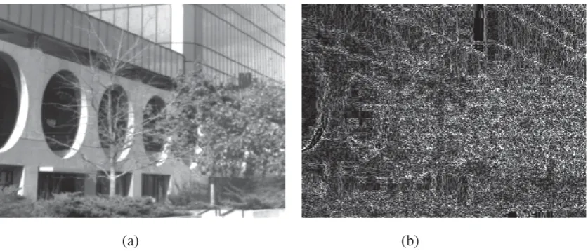
A black and white photograph of a poster was taken with a 5 megapixel digital camera and a section (320x240) was cropped from this photograph to show only the area of interest shown in Figure 3(a). The image was saved as BUILDING.TIF and required a memory space of about 82 KB. An image thus obtained was considered to be an image that would preserve the basic integrity of its gray scale information, and could then be used for statistical purposes.
A second image of the BUILDING was obtained by compressing the BUILDING.TIF file using a JPEG standard of compression and a DCT (Discrete Cosine Transform) decorrelator. The size of this BUILDING.JPEG image was also 320x240 and the storage capacity requirement of about 10 KB for a compression ratio of approximately 8.
In order to compare these two images statistically they were subtracted and the differences used to compute the overall root-mean square (r.m.s.) of +/- 9.77 intensity values, with maximum and minimum differences of +49 and -35 respectively. These figures are just indicative of the amount of information that may be lost when an image is compressed. Figure 3(b) shows graphically the results of subtracting the original .TIF image file and its compressed JPEG version.
The main drawback of algorithms with a DCT basis is that each 8x8 block of a given image is coded independently from its neighbours. This creates problems of continuity between blocks after decompression. This occurrence is referred to as the blocking effect, but it may be invisible to the eye for low compression ratios (< 4). The blocking effect is especially obvious in flat areas of an image (Gonzalez and Woods, 2007).
(a) (b)
Fig. 3: (a) The original BUILDING.TIF file and (b) an image of differences between BUILDING.TIF and its .JPEG compressed version.
[image:6.595.89.508.460.639.2]583
BUILDING.TIF was +/- 8.22 pixels intensity values with maximum and minimum differences of +31 and -28 respectively. These figures were obtained for a grid ratio of 5.0 and represent a 15% improvement in the r.m.s. values obtained previously by subtracting the original image BUILDING.TIF and its compressed version BUILDING.JPEG.
(a) (b)
[image:7.595.87.510.126.300.2]Fig. 4: (a) One of the 100 downsampled and compressed images (64x48) used to reconstruct the image (320x240) in (b), for a grid ratio equal to 5.0.
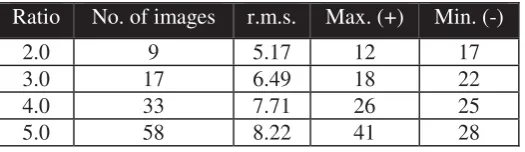
Table 1 indicates the number of images that were required to reconstruct an enhanced composite of the BUILDING (320x240) for varying grid ratios. From this table it appears evident that the required number of low-resolution images to fill one high-resolution image increases exponentially as the grid ratio increases linearly. Adding more images to this process did not improve significantly the r.m.s. results. In this controlled experiment the number of images required to solve for a given grid ratio could be approximated to 2p2 (p is the grid ratio). In addition, the accuracy of the reconstruction process deteriorates as the grid ratio increases.
The reconstruction of a digital image with the minimum number of low-resolution images is possible, but it should not be expected to always achieve a high accuracy, especially for high grid ratios (i.e., >4). High grid ratios require large numbers of low-resolution images, meaning that these low-resolution images must be relatively close to one another. This implies the detection of image shifts whose dimensions may be lower than the actual accuracy achievable by the sub-pixel registration process (i.e., 0.1 pixels). Hence, it is important that the distribution of the computed shifts between the low-resolution images be as complete and as far apart as possible.
Ratio No. of images r.m.s. Max. (+) Min. (-)
2.0 9 5.17 12 17
3.0 17 6.49 18 22
4.0 33 7.71 26 25
5.0 58 8.22 41 28
Tab. 1: r.m.s. of differences of pixels intensities between the original image BUILDING.TIF and the image composites reconstructed using low-resolution images and compressed images for varying grid ratios.
[image:7.595.168.431.545.621.2]584
potential noise and where the computed sub-pixels image shifts rather than pre-assigned shifts are used.
IMAGE ENHANCEMENT AND NOISE
If an image is acquired directly in a digital format, the mechanism for gathering the data (such as a CCD detector) can introduce noise. Specific types of noise models in images is beyond the scope of this paper and further information on noise patterns and characteristics can be found in (Russ, 2007). In order to establish the number of images needed to reconstruct a high-resolution image of the BUILDING in the presence of potential noise and computed sub-pixel registrations, the proposed enhancement algorithm was repeated in a second test in which random 'salt & pepper' noise was added to each of the images of the low-resolution data sets used in the first experiment.
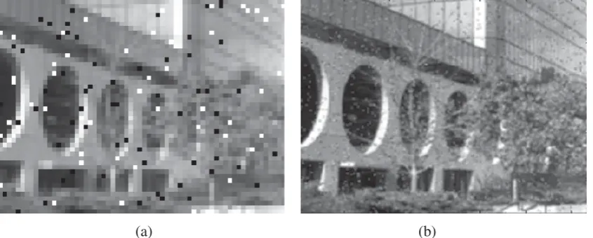
The percentage of the total number of pixels (typically 1%, 3% and 5%) was changed to either totally black or white. The effect is similar to sprinkling white and black dots on the image as shown in Figure 5(a). The figure relates to a grid ratio equal to 5.0 with 5% added random noise. One example where salt and pepper noise arises is in transmitting images over noisy digital links (Chapman and Chapman, 2000).
(a) (b)
Fig. 5: (a) one of the 100 degraded (64x48), noisy and compressed images used to reconstruct the enhanced composite in (b) (320x240).
In this second test the calculated shifts between images, rather than the known shifts, were used. All the possible combinations of these shifts were computed, and the median was adopted in the mapping of the low-resolution pixels onto each high-resolution grid system. Table 2 shows the results of the differences between the sub-pixel shifts of the low-resolution and noisy images as compared to the known shifts (for space limitations only the results for 5 images are shown in Table 2). Although the data in this table relate to a grid ratio equal to 5.0 (the worst case scenario) very similar yet proportional results were found for the other ratios (i.e., 2.0, 3.0, 4.0).
[image:8.595.89.512.344.514.2]585
Table 3 indicates the number of images that were actually required to optimise the reconstruction of an enhanced composite of the BUILDING (320x240) for the various grid ratios. Similarly to the results of Table 1 the required number of low-resolution images to fill one high-resolution image increases exponentially as the grid ratio increases linearly.
Noise 0% Noise 1% Noise 3% Noise 5%
Images dx dy dx dy dx dy dx dy 1 0.000 0.000 0.000 0.000 0.000 0.000 0.000 0.000 2 0.005 0.009 0.018 0.021 0.008 0.037 0.018 0.093 3 0.016 0.003 0.029 0.060 0.012 0.065 0.032 0.107 4 0.020 0.021 0.032 0.024 0.050 0.060 0.047 0.092 5 0.008 0.030 0.030 0.027 0.028 0.037 0.083 0.111 … … … … r.m.s 0.011 0.018 0.027 0.032 0.054 0.045 0.063 0.081
Tab. 2: Sub-pixel shift differences from true with increased noise (grid ratio p=5.0).
Ratio (p) No. of images r.m.s. Max. (+) Min. (-)
2 19 10.17 23 27
3 40 12.49 48 33
4 69 13.08 63 47
5 104 15.22 71 54
Tab. 3: r.m.s. of differences of pixels intensities between the original image BUILDING.TIF and the image composites reconstructed using low-resolution, compressed and noisy images for increasing grid ratios.
From table 3 the number of images required to solve for a given grid ratio could be approximated to 4p2. Beyond this number of images no improvement was observed in the r.m.s. In addition, the accuracy of the reconstruction process deteriorates sharply as the grid ratio increases. It should be noticed that the enhancement process is also responsible for reducing or attenuating noise, that is, the pronounced grainy appearance present in the low-resolution images (see the images in Figure 5).
The accuracy of the enhancement for varying levels of random noise and solving for an enhanced image across a range of grid ratios determined that not only the level of noise present in the images affected the accuracy of the enhancement, but also the size of the grid ratio being applied was relevant. As the grid ratio increased from 2.0 to 5.0, the accuracy of the enhancement was increasingly degraded (see Table 3).
The tests of this section could have been carried out by first removing the noise from the low-resolution and degraded images using a dedicated filter (i.e., a median filter). Indeed, there are number methods for noise removal presented in the literature (Russ, 2007). However, the sequential application of one of these filters followed by a SR technique rarely provides good results (Tom and Katsaggelos, 2001). It is suggested that information removed during pre-processing might have been useful for resolution enhancement.
CONCLUSIONS
586
The amount of noise in the low-resolution images affects the precision of the resultant enhanced image. However, the precision and accuracy of the results can be improved by using more than the minimum required number of low-resolution images in order to reconstruct a higher-resolution composite.
Although the number of low-resolution images is unlimited, tests results indicated that using a number of low-resolution images greater than 4p2 (p=grid ratio) would not improve significantly the accuracy of the enhanced composite.
The image registration process can accurately determine the relative shifts between two images. However, changing and repeating the procedure using different reference frames may determine improved estimates of such shifts.
To minimise the influence of noise, it is important that the distribution of the shifts between the low-resolution images to be as representative and as far apart as possible.
As the grid ratio increases, the accuracy of the final enhanced composite decreases.
The proposed enhancement process can reconstruct high-resolution image with a substantial attenuation of JPEG compression artefacts (i.e. blocking effects).
Refinements to the proposed algorithm are being undertaken to increase the accuracy achievable for larger grid ratios (>5.0) and the inclusion of rotation within the degraded input images. To extend the range of applications that could benefit from utilising this device independent algorithm is another goal. In addition, the author is currently investigating the possibility of adapting this enhancement process to a generalized scheme whereby both sensor and object are dynamic and the illumination is non-uniform.
REFERENCES
Chpaman N. and Chapman J., 2000 “Digital Multimedia”. John Wiley and Sons, Ltd. 568 pages.
Farsiu S., Robinson D., Elad M., and Milanfar P., 2004 “Advances and Challenges in SR", International Journal of Imaging Systems and Technology, Volume 14, no 2, pp. 47-57, August. Fryer J. and McIntosh, K.L. , 2001. “Enhancement of Image Resolution in Digital Photogrammetry”. Photogrammetric Engineering & Remote Sensing”, Vol.67, No.6, pp.741-749.
Gonzalez R.C. and Woods R.E. (2007) “Digital image processing” Edition: 3, Published by Prentice Hall. 954 pages.
Hendriks L. C. and van Vliet L.J., 1999. “Resolution Enhancement of a Sequence of Undersampled Shifted Images”. ASCI 1999. Proceeding 5th Annual Conference of the Advanced School for Computing and Imaging (Heijen. NL. June 15-17). ASCI. Delft. 95-102. Petrie, G. and Kennie, T.J.M., 1990. Terrain Modelling in Surveying and Civil Engineering. Whittles, Caithness, Scotland and Thomas Telford. 351 pages.
Pilgrim, L.J., 1991. Simultaneous Three Dimensional Object Matching and Surface Difference Detection in a Minimally Restrained Environment. Research Report No. 066.08.1991. University of Newcastle, NSW, Australia. 215 pages.
Russ C. J., 2007 “The Image Processing Handbook”, Published by CRC Press, ISBN 0849372542, 9780849372544, 817 pages.
Scarmana G. and Fryer J., 2006. “Enhancing a Sequence of Facial Images by Combining Multiple Under-sampled and Compressed Images”. The Photogrammetric Record 21(114): 1– 13, June.
Spiegel M. R. and Stephens L., 1999. “Theory and Problems of Statistics”, Schaum’s Outline Series, McGraw-Hill Book Company”. pp. 556.
587
Vandewalle P., Susstrunk S. and Vetterli M., 2005. A Frequency Domain Approach to Registration of Aliased Images with Application to SR, EURASIP Journal on Applied Signal Processing (special issue on SR).
Wolf, P. R. and Dewitt, B.A., 2000. Elements of Photogrammetry with Applications in GIS. Third Edition, McGraw Hill. 608 pages: 307-325.
Zhouchen, L. and Heung-Yeung, S., 2004. Fundamental limits of Reconstruction-Based SR Algorithms under Local Translation. IEEE Transactions on Pattern Analysis and Machine Intelligence. Vol. 26, No.1, January.
AUTHOR’S BIOGRAPHY