A multidomain integrated-radial-basis-function collocation method for elliptic problems

A multidomain integrated-radial-basis-function

collocation method for elliptic problems

N. Mai-Duy

and T. Tran-Cong

Faculty of Engineering and Surveying,

The University of Southern Queensland, Toowoomba, QLD 4350, Australia

Submitted to

Numerical Methods for Partial Differential Equations,

11-Jul-2007; revised, 11-Oct-2007

∗_{Corresponding author: Telephone +61 7 4631 1324, Fax +61 7 4631 2526, E-mail}

Abstract This paper is concerned with the use of integrated radial-basis-function networks (IRBFNs) and non-overlapping domain decompositions (DDs) for

numer-ically solving one- and two-dimensional elliptic problems. A substructuring

tech-nique is adopted, where subproblems are discretized by means of one-dimensional

IRBFNs. A distinguishing feature of the present DD technique is that the

continu-ity of the RBF solution across the interfaces is enforced with one order higher than

with conventional DD techniques. Several test problems governed by second- and

fourth-order differential equations are considered to investigate the accuracy of the

proposed technique.

KEY WORDS: non-overlapping domain decomposition; radial basis function;

collo-cation technique; high-order differential equations

1

Introduction

The basic idea of a physical DD technique (cf. [1]) is to divide the problem domain

into a number of subdomains, on which the governing differential equations (DEs)

are solved with transmission conditions at the interfaces. The main advantage of

DD techniques lies in their ability to handle large-scale problems. Given a spatial

discretization, the size of matrices obtained with DD techniques is much smaller

than that with a one-domain technique. With the recent emergence of parallel

com-puters, DD techniques have become more attractive because they allow the parallel

computations of solutions to subdomains. The disadvantage of DD techniques is

that their solution is not as smooth as that on a single domain.

The basic part of any DD technique lies in the method of matching the computed

order are enforced across the subdomain interfaces. For second-order problems, the

enforcement is applied to the solution and its first-order normal derivative, while for

fourth-order problems, one imposes the continuity for the solution and its normal

derivatives of order up to three. The DD approach thus provides an approximate

solution that is aC1 _{function across the interfaces for second-order problems andC}3

function for fourth-order problems. It is noted that there are relatively few papers

on DDs for the solution of fourth-order differential problems.

RBF collocation methods for solving DEs appeared in the early 1990s. Kansa [2] and

Fasshauer [3] were the first to suggest the so-called non-symmetric and symmetric

RBF collocation methods, respectively. The RBF methods are easy to implement

and have the capability to provide a very accurate solution using relatively low

numbers of points. When handling large-scale problems, like other discretization

techniques, the RBF methods need to be combined with DD techniques for an

efficient solution or one needs to construct the RBF approximations locally. A

number of RBF papers discussing these topics have been reported, see, e.g. [4-8] for

the use of DDs and [9-11] for the use of local approximations. A drawback of the

DD approach is that it requires a domain partition, i.e. some sort of meshing. For

these one- and multi-domain RBF collocation techniques, the construction of the

RBF approximations is based on differentiation (DRBFNs).

In this paper, we discuss a multidomain IRBFN collocation technique for the solution

of second- and fourth-order elliptic problems in one and two dimensions. The IRBFN

discretization scheme, which is applied on subdomains here, is based on the use

of a Cartesian grid and a one-dimensional (1D) IRBFN interpolation scheme that

has recently been reported in [12,13]. The incorporation of 1D-IRBFNs into the

substructuring technique leads to an approximate solution that is a Cp _function,

instead of the usual Cp−1, across the subdomain interfaces, where p is the order

approximate solution alleviates the deterioration in accuracy caused by the domain

division.

An outline of the paper is as follows. Brief reviews of 1D-IRBFNs for the

approxima-tion of funcapproxima-tions and the soluapproxima-tion of DEs are given in Secapproxima-tions 2 and 3, respectively.

The proposed DD technique is described in Section 4. Numerical results are

pre-sented in Section 5. Section 6 concludes the paper.

2

A brief review of 1D-IRBFNs

Consider a univariate functionf(x). The basic idea of the integral RBF scheme [14]

is to decompose a pth-order derivative of the functionf into RBFs

dp_f(x)

dxp = n

X

i=1

wiϕi(x) = n

X

i=1

wiIi(p)(x), (1)

where{wi}n_i=1 is the set of network weights, and{ϕi(x)}n_i=1 ≡

n

I_i(p)(x)on

i=1 is the set

of RBFs. Lower-order derivatives and the function itself are then obtained through

integration

dp−1f(x)

dxp−1 =

n

X

i=1

wiIi(p−1)(x) +c1, (2)

dp−2f(x)

dxp−2 =

n

X

i=1

wiIi(p−2)(x) +c1x+c2, (3)

· · · ·

df(x)

dx =

n

X

i=1

wiIi(1)(x) +c1

xp−2

(p−2)! +c2

xp−3

(p−3)! +· · ·+cp−2x+cp−1, (4)

f(x) =

n

X

i=1

wiIi(0)(x) +c1

xp−1

(p−1)! +c2

xp−2

where I(p−1)

i (x) =

R

I_i(p)(x)dx, I(p−2)

i (x) =

R

I(p−1)

i (x)dx,· · · , I

(0)

i (x) =

R

I_i(1)(x)dx, and c1, c2,· · · , cp are the constants of integration.

Unlike conventional differential schemes, the starting point of the integral scheme

can vary in use, depending on the particular application under consideration. The

scheme is said to be of order p, denoted by IRBFN-p, if the pth-order derivative is taken as the starting point.

The evaluation of (1)-(5) at a set of collocation points{xj}n_j=1 leads to

d

dp_f

dxp =Ib

(p)

[p]α,b (6)

d

dp−1f

dxp−1 =

b I(p−1)

[p] α,b (7)

· · · ·

cdf dx =Ib

(1)

[p]α,b (8)

b

f =Ib_[(0)_p]α,b (9)

where the subscript [.] and superscript (.) are used to denote the order of the

IRBFN scheme and the order of a derivative function, respectively;

b I_[(_pp_]) =

        

I₁(p)(x1), I2(p)(x1), · · · , In(p)(x1), 0, 0, · · · , 0, 0

I₁(p)(x2), I2(p)(x2), · · · , In(p)(x2), 0, 0, · · · , 0, 0

· · · ·

I1(p)(xn), I2(p)(xn), · · · , In(p)(xn), 0, 0, · · · , 0, 0

         , b I(p−1)

[p] =

        

I(p−1)

1 (x1), I2(p−1)(x1), · · · , In(p−1)(x1), 1, 0, · · · , 0, 0

I(p−1)

1 (x2), I2(p−1)(x2), · · · , In(p−1)(x2), 1, 0, · · · , 0, 0

· · · ·

I(p−1)

1 (xn), I2(p−1)(xn), · · · , In(p−1)(xn), 1, 0, · · · , 0, 0

· · · ·,

b I_[(0)_p] =

        

I₁(0)(x1), I2(0)(x1), · · · , In(0)(x1), x

p−1

1

(p−1)!,

xp−2

1

(p−2)!, · · · , x1, 1

I₁(0)(x2), I2(0)(x2), · · · , In(0)(x2), x

p−1

2

(p−1)!,

xp−2

2

(p−2)!, · · · , x2, 1

· · · ·

I₁(0)(xn), I2(0)(xn), · · · , In(0)(xn), x

p−1

n

(p−1)!,

xp−2

n

(p−2)!, · · · , xn, 1

         ; b

α= (w1, w2,· · · , wn, c1, c2,· · · , cp)T ;

and

d

dk_f

dxk =

dk_f

1

dxk,

dk_f

2

dxk,· · · ,

dk_f n

dxk

T

, k = (1,2,· · · , p),

b

f = (f1, f2,· · · , fn)T ,

in whichdk_f

j/dxk =dkf(xj)/dxk and fj =f(xj) with j = (1,2,· · · , n).

The use of integrated basis functions is expected to avoid the problem of reduction of

convergence rate caused by differentiation [15]. Numerical studies (e.g. [16,17]) have

shown that the integral collocation approach is more accurate than the differential

one. Recently, theoretical studies [18] have confirmed superior accuracy of IRBFNs

over DRBFNs. Moreover, there are additional weights (integration constants) in the

integral collocation formulation, and they have been found to be extremely useful

for handling the multiple boundary conditions [19-21]. This study further exploits

the constants of integration for the purpose of improving the order of continuity of

3

A brief review of 1D-IRBFNs for solving DEs

on a single domain

In the remainder of the paper, we will use

• the notation b[] for a vector/matrix [] that is associated with a grid line,

• the notation e[] for a vector/matrix [] that is associated with the whole set of

grid lines,

• the notation [] for a vector/matrix [] that is associated with the boundaries

of the domain,

• the notation [](η,θ) to denote selected rows η and columns θ of the matrix [],

• the notation [](η) to pick out selected components η of the vector [],

• the notation [](:,θ) to denote all rows of the matrix [], and

• the notation [](η,:) to denote all columns of the matrix [].

3.1

1D elliptic problems

Consider a 1D boundary-value problem governed by thepth-order ODE

F(u,du dx,

d2_u

dx2,· · · ,

dp_u

dxp) =b(x), r≤x≤s, (10)

where F and b are prescribed functions, together with boundary conditions for u,

du/dx, ..., and dp/2−1u/dxp/2−1 atx=r and x=s.

The continuous domain of interest is replaced by a set of discrete points{xj}n_j=1with

to approximate the field variable and its derivatives in the ODE and the boundary

conditions. Owing to the presence ofp integration constants in the integral

formu-lation, one can addp extra equations to the discrete system. These extra equations

can be utilized to represent the ODE and the values of the derivative boundary

con-ditions at both ends of the domain. The governing equation (10) and the boundary

conditions can be transformed into the following discrete form

b

Aαb=f ,b (11)

whereAbis the system matrix of size (n+p)×(n+p) defined as

b A=                       

F Ib_[(0)_p](1,:),Ib_[(1)_p](1,:),Ib_[(2)_p](1,:),· · · ,Ib_[(_pp_](1) _,:)

F Ib_[(0)_p](2,:),Ib_[(1)_p](2,:),Ib_[(2)_p](2,:),· · · ,Ib_[(_pp_](2) _,:) · · ·

F Ib_[(0)_p](n,:),Ib_[(1)_p](n,:),Ib_[(2)_p](n,:),· · · ,Ib_[(_pp_]()_n,:) b

I_[(0)_p]([1,n],:)

b

I_[(1)_p]([1,n],:)

· · ·

b I(p/2−1)

[p]([1,n],:)

                       , b

α= (w1, w2,· · · , wn, c1, c2,· · · , cp)T, and

b

f = (b1, b2,· · · , bn, ur, us,

dur

dx , dus

dx,· · · ,

dp/2−1u

r

dxp/2−1 ,

dp/2−1u

s

dxp/2−1 )

T_.

In (11), the ODE is collocated at the whole set of grid points including the two

boundary pointsx=r and x=s. Solving (11) yields

b

α=Ab−1_{f ,}b ₍₁₂₎

3.2

2D elliptic problems

Consider a 2D boundary value problem governed by thepth-order PDE

F(u,∂u ∂x,

∂u ∂y,· · · ,

∂k_u

∂xi_∂yj,· · · ,

∂p_u

∂xp,

∂p_u

∂yp) = b(x, y), (x, y)∈Ω, (13)

where Ω is a rectangular domain, and subject to the prescribed conditions for u,

∂u/∂n, ..., and ∂p/2−1u/∂np/2−1 on the boundaries of Ω (n−the direction normal to

the boundary).

The 1D-IRBFN-based Cartesian-grid technique approximates the solution in terms

of nodal variable values rather than network weights. On a grid line, thepth-order

integral scheme (IRBFN-p) is employed. Along a horizontal grid line, the

relation-ships between the network-weight space and the physical space can be described

by _



 ub

b

v

 

=Cb[p] α,b (14)

whereCb[p] is the conversion matrix of dimension (nx+p)×(nx+p)

b C[p]=

            b I_[(0)_p]

b

I_[(1)_p]([1,nx],:)

· · ·

b I(p/2−1)

[p]([1,nx],:)

b

I_[(_pp_]([1) _,nx],:)             , b

u= (u1, u2,· · · , unx)

T , b v = ∂u1 ∂x , ∂unx

∂x ,· · ·,

∂p/2−1u

1

∂xp/2−1 ,

∂p/2−1u

nx

∂xp/2−1 ,

∂p_u

1

∂xp ,

∂p_u nx

∂xp

T

,

b

α= (w1, w2,· · · , wnx, c1, c2,· · · , cp)

T

and nx is the number of grid points on the line. It can be seen that (14) takes into

account information about the values ofuat the grid points (the first nx equations),

the derivative boundary conditions (the next (p−2) equations) and the PDE at the

boundary points (the last two equations). Solving (14), one will obtain a map from

the physical space to the network-weight space

b

α=Cb−1

[p]

 

 ub

b

v

 

. (15)

Substitution of (15) into (6)-(8) yields

d

∂k_u

∂xk =Ib

(k) [p]Cb

−1

[p]

 

 bu

b

v

 

, k= (1,2,· · · , p), (16)

where ∂_∂xckuk =

∂k_u

1

∂xk ,

∂k_u

2

∂xk,· · · ,

∂k_u nx

∂xk

T

. Approximate expressions for derivatives ofu

with respect to x over the whole domain can then be conveniently constructed by

means of Kronecker tensor products. The process of constructing the 1D-IRBFN

approximations for∂k_u/∂yk _{is similar to that for ∂}k_u/∂xk_.

Moreover, mixed derivatives ofu can be computed via the following relation

∂k_u

∂xi_∂yj =

1 2 ∂i ∂xi

∂j_u

∂yj + ∂ j ∂yj

∂i_u

∂xi

, with k =i+j, (17)

which reduces the computation of mixed derivatives to that of lower-order pure

derivatives for which IRBFNs involve integration with respect to x or y only. In

computing (17), lower-order integral schemes are employed, and hence one only

needs to take derivative boundary conditions (not information about the PDE at

Letn, nip and nbp be the total number of collocation points, the number of interior

points and the number of boundary points, respectively. Collocating (13) at the

interior points results in

e A             e u ∂u ∂n · · ·

∂p/2₋1

u ∂np/2₋1

∂p_u

∂np            

=eb, (18)

where Aeis a known matrix of size nip×(n+ (p/2)nbp);eb represents the values of

b in (13) at the interior points; ue = (u1, u2,· · ·, un)T; and _∂n∂u,· · · ,∂

p/2₋1_u

∂np/2₋1 and

∂p_u

∂np

represent the values of ∂u_∂n,· · · ,∂p/2−1_u

∂np/2

−1 and

∂p_u

∂np at the boundary points, respectively.

The equation set (18) can be rewritten as

e

A(:,ip) ue(ip)=eb− B0u− B1

∂u

∂n +· · · − Bp/2−1

∂p/2−1u

∂np/2−1 − Bp

∂p_u

∂np, (19)

where

u=ue(bp), B0 =Ae(:,bp),

B1 =Ae(:,n+bp),· · · , Bp/2−1 =Ae(:,n+nbp(p/2−2)+bp), Bp =Ae(:,n+nbp(p/2−1)+bp),

and the notations ip and bp refer to the indices of the rows/columns that are

as-sociated with the interior and boundary points, respectively. Given the PDE and

the boundary conditions, the right-hand side of (19) can reduce to a known vector.

In forming (19), the IRBFN discretization does not involve the four corners of the

domain.

More details can be found in [12]. In the case of irregular domains, there are some

4

The proposed multidomain(MD) IRBFN method

The present DD method is based on the use of non-overlapping subdomains and

1D-IRBFNs. The substructuring technique is employed to construct a separated

problem that involves the unknowns relative to the subdomain interfaces only (the

Schur complement system). Subdomains are handled here with the

1D-IRBFN-based Cartesian-grid method.

4.1

1D elliptic equations

For simplicity, the present DD technique is described for the case of the biharmonic

equation and 2 non-overlapping subdomains, namelyI and II. The values of uand

du/dxat the interface ˇx are selected to be the interface unknowns

uI(ˇx) =uII(ˇx) = ˇu, (20)

duI

dx(ˇx) = duII

dx (ˇx) =

ˇ

du

dx, (21)

and these unknowns are then determined by solving the equations of continuity in

second- and third-order derivatives

d2_u

I

dx2 (ˇx) =

d2_u

II

dx2 (ˇx), (22)

d3_u

I

dx3 (ˇx) =

d3_u

II

Expressions for d2_u/dx2 _{and d}3_u/dx3 _{in the Schur complement system, (22) and}

(23), are constructed using the subdomain solver ((10)-(12))

d2_u

dx2(ˇx) = Ib (2)

[4](n,:)αb=Ib (2) [4](n,:)Ab−

1_{f ,b (24)}

d3_u

dx3(ˇx) = Ib (3)

[4](n,:)αb=Ib (3) [4](n,:)Ab−

1_{f ,b (25)}

in whichfb=b1, b2,· · · , bn, ur,u,ˇ du_dxr,du_dxˇ

T

for subdomain I, and

d2_u

dx2(ˇx) =Ib (2)

[4](1,:)αb=Ib (2) [4](1,:)Ab

−1f ,b (26)

d3_u

dx3(ˇx) =Ib (3)

[4](1,:)αb=Ib (3) [4](1,:)Ab−

1_{f ,b (27)}

in which fb = b1, b2,· · · , bn,u, uˇ s,du_dxˇ,du_dxs

T

for subdomain II. In (24)-(27), the

subscripts I and II are dropped out for brevity.

Substitution of (24)-(27) into (22)-(23) leads to a set of two algebraic equations for

the two unknowns ˇuand ˇdu_dx. Once these unknowns are determined, the solutions to subdomains will be obtained through (12) and (6)-(9).

A distinguishing feature of the present DD scheme is that, in solving a subproblem,

the ODE is forced to be satisfied exactly at the interface (thenth and 1st rows in

(11) for subdomains I and II, respectively):

d4_u

I

dx4 (ˇx) +

d2_u

I

dx2 (ˇx) = b(ˇx) and (28)

d4_u

II

dx4 (ˇx) +

d2_u

II

dx2 (ˇx) = b(ˇx). (29)

Since the field variableuand its first three derivatives are enforced to be continuous at the interface ((20)-(23)), equations (28) and (29) lead to

d4_u

I

dx4 (ˇx) =

d4_u

II

The present MD-IRBFN technique thus achieves aC4 _{solution at the interface.}

4.2

2D elliptic equations

The MD-IRBFN method in the previous section is extended to the case of

two-dimensional problems. The problem domain, which can be of regular and irregular

shape, is partitioned into a number of subdomains, for which the interfaces are

required to run parallel to the x and y axes and the grid points on the interface of

two adjoining subdomains are chosen to be the same. The MD-IRBFN method is

described in detail for the Poisson and biharmonic equations with Dirichlet boundary

conditions. Special attention is given to the treatment for the continuity of the

approximate solution at the interior corner points.

4.2.1 Poisson equation

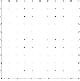
Consider a typical subdomain (i.e. all boundaries are the interfaces) (Figure 1). The

proposed DD technique gives different treatments for the interior corner points (the

intersection points) and the interior points on the interfaces (the interface points),

which achieves a C2 _{solution across the interfaces. The present Schur complement}

system is constructed as follows. The unknown values on the interfaces are chosen to

be the values ofu at the interface points and the values ofu, ∂2_u/∂x2 _{and ∂}2_u/∂y2

at the intersection points. The equations used for determining these unknowns are

based on the continuity of ∂u/∂n at the interface points, and the continuity of

∂u/∂x, ∂u/∂y together with the satisfaction of the PDE at the intersection points.

First, one needs to express the values ofu at the interior points of a subdomain in terms of the interface unknowns only. For the Poisson equation, the discrete system

(19) reduces to

e

A(:,ip) eu(ip) =eb− B0u− B2

∂2_u

∂n2. (31)

The second-order normal derivative vector on the right-hand side of (31) can be

replaced by

∂2_u

∂n2 =b−

∂2_u

∂t2, (32)

wheret is the direction tangent to the boundary.

We employs the second-order integral scheme (IRBFN-2) to express tangent

deriva-tives in (32) in terms of the interface unknowns. For an interface of the subdomain,

one has

d

∂2_u

∂t2 =Ib (2) [2]Cb−

1 [2]

 

 ub

b

v

 

, (33)

where _bu represents the values of u at the grid points on the interface, and _bv the

values of ∂2_u/∂t2 _{at the two extreme points of the interface (i.e. the intersection}

points).

Second, by taking (31), (32) and (33) into account, one is able to derive the values

of ∂u/∂nat the interface points in terms of the interface unknowns only.

Intersection points: The values of ∂u/∂x and ∂u/∂y at these nodes are simply computed via function approximation.

obtains the values of ∂u/∂x at the intersection points    ∂u1 ∂x ∂unx ∂x  

=Ib_[2]([1(1) _,nx],:)Cb−1

[2]       b u ∂2 u1 ∂x2 ∂2 unx ∂x2     

, (34)

whereu_brepresents the values of u at the grid points on the interface.

Similarly, for the interfaces that run parallel to they axis, one has

   ∂u1 ∂y ∂uny ∂x  

=Ib_[2]([1(1) _,ny],:)Cb−1

[2]       b u ∂2 u1 ∂y2 ∂2 uny ∂y2     

. (35)

The computations here are relatively simple because the approximations used involve

information about the interfaces only.

The third equation in a set of three equations, which is employed at each intersection

point, is the PDE in its original form, i.e.

∂2_u

∂x2 +

∂2_u

∂y2 =b. (36)

Owing to the fact that the PDE is not collocated at the four corners of the domain in

the solution of subdomains, equation (36) is independent from continuity equations

for∂u/∂n.

Continuity order: The present DD technique enforces the continuity of the solu-tion across the interfaces with one order higher than convensolu-tional DD techniques

because (i) the PDE is forced to be satisfied at the interface points in the

4.2.2 Biharmonic equation

The MD-IRBFN method for the biharmonic equation is similar to that for the

Poisson equation. However, the Schur complement system is larger. The unknown

vector consists of the values ofuand∂u/∂nat the interface points, and the values of

u,∂u/∂x,∂u/∂y,∂4_u/∂x4 _and∂4_u/∂y4 _{at the intersection points. The construction}

of the interface system is based on the use of a set of two equations, namely∂2_u/∂n2

and ∂3_u/∂n3_{, at an interface point, and a set of 5 equations, ∂}2_u/∂x2_{, ∂}2_u/∂y2_,

∂3_u/∂x3_{, ∂}3_u/∂y3 _{and the PDE, at an intersection point.}

The values of ∂2u/∂n2 and ∂3u/∂n3 at an interface point are computed using the

subdomain solver and the IRBFN-4 scheme. The equations that correspond to (31),

(32) and (33) are, respectively,

e

A(:,ip) eu(ip) =eb− B0u− B1

∂u ∂n− B4

∂4_u

∂n4, (37)

∂4_u

∂n4 =b−2

∂4_u

∂x2_∂y2 −

∂4_u

∂t4, (38)

d

∂4_u

∂t4 =Ib (4) [4] Cb

−1

[4]

 

 ub

b

v

 

, (39)

where_bv consists of the values of∂u/∂tand∂4_u/∂t4 _{at the intersection points. After}

solving (37), any derivative functions of u, including the mixed fourth-order one,

can be expressed in terms of the interface unknowns only.

On the other hand, the computation of∂2_u/∂x2_{, ∂}2_u/∂y2_{, ∂}3_u/∂x3 _{and ∂}3_u/∂y3 _at

an intersection point is based on the use of the fourth-order 1D-IRBFN scheme only.

points of the interface are given below    ∂2 u1 ∂x2 ∂2 unx ∂x2  

=Ib_[4]([1(2) _,nx],:)Cb−1

[4]             b u ∂u1 ∂x ∂unx ∂x ∂4 u1 ∂x4 ∂4 unx ∂x4             and (40)    ∂3 u1 ∂x3 ∂3 unx ∂x3  

=Ib_[4]([1(3) _,nx],:)Cb−1

[4]             b u ∂u1 ∂x ∂unx ∂x ∂4 u1 ∂x4 ∂4 unx ∂x4             , (41)

whereu_bis the vector containing the values of uat the grid points on the interface.

Continuity order: Consider an interface (Γ) and its two associated subdomains

(Ω1 and Ω2). As shown earlier, the present DD technique imposes the

continu-ity for the solution u and its normal derivatives of order up to four (i.e. ∂u/∂n,

∂2_u/∂n2_{, ∂}3_u/∂n3 _{and ∂}4_u/∂n4_{) at every point on the interface Γ. The 1D-IRBFN}

approximations for derivatives of these interface values with respect to the tangent

direction (i.e. mixed derivatives) from subdomain Ω1 can be seen to be identical to

those taken from subdomain Ω2. In other words, one also has the continuity across

the interface Γ for mixed derivatives (e.g. ∂4_u/∂t2_∂n2_{). The present DD technique}

5

Numerical examples

Several examples are presented here to demonstrate the attractiveness of the

pro-posed DD technique.

It has generally been accepted that, among RBFNs, the multiquadric (MQ)-based

interpolation scheme tends to result in the most accurate results. The present

1D-IRBFN schemes are implemented with the MQ function whose form is

ϕi(x) =

q

(x−ci)2 +a2i, (42)

where ci and ai are the centre and the width of the ith MQ function, respectively.

The centre points are selected to coincide with the collocation points. The MQ

widths are known to have a profound effect on the performance of MQ-RBFNs.

However, there is still a lack of mathematical theories for specifying their optimal

values. For all numerical examples taken here, the MQ widths are simply computed

by

ai =βdi, i= (1,2,· · · , n), (43)

in whichβ is a factor anddi is the distance between the theith centre and its closest

neighbour. The reader is referred to [16,19] for a discussion about the effect ofβ on accuracy of the RBFN solutions.

To assess the accuracy of the IRBFN method, the one-domain IRBFN and

MD-DRBFN methods are considered. It is noted that the present MD-MD-DRBFN method

is also based on the substructuring technique and the multiquadric functions. Both

5.1

1D second-order problem

Consider the following second-order ODE

d2_u

dx2 +

du

dx+u=−exp(−5x) [9979 sin(100x) + 900 cos(100x)], 0≤x≤1, (44)

with Dirichlet boundary conditions u(0) = 0 and u(1) = sin(100) exp(−5). The

exact solution can be verified to be

ue(x) = sin(100x) exp(−5x), (45)

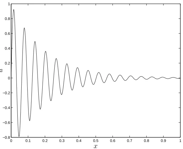
which is highly oscillatory as shown in Figure 2.

The domain is partitioned into two subdomains of the same size, and each subdomain

is discretized with uniformly distributed points. Twenty grids are considered with

their densities varying from 11 to 201 in increment of 10. The accuracy of a numerical

scheme is measured by means of the discrete relative L2 norm of the solution (Ne).

A test set of 201 uniform points is used to compute the error Ne.

The approximate solution is aC1 _{function across the interface for MD-DRBFNs and}

C2 _{for MD-IRBFNs.}

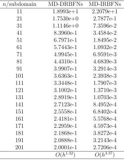
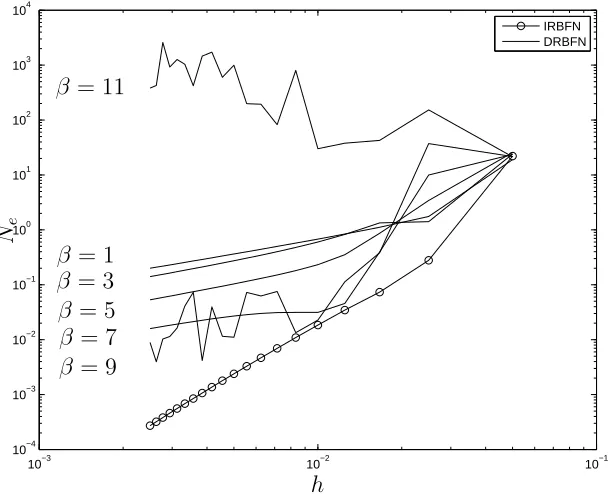
Table 1 presentsNes of MD-DRBFNs and MD-IRBFNs obtained with β = 1. The

performance of the latter is far superior to that of the former in both accuracy and

convergence rate. The MD-DRBFN results are relatively poor. As mentioned earlier,

the RBF widths strongly affect the accuracy of RBFNs. Figure 3 shows a significant

improvement in accuracy for MD-DRBFNs with increasing RBF widths. However,

the MD-DRBFN results with higher values ofβ are still less accurate than the

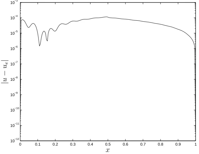
becomes unstable for β = 9 and there is no grid convergence observed for β = 11. We also investigate how the domain partition affects the local error. Figure 4 shows

the variation of the absolute error of the MD-IRBFN solution over the domain. It

can be seen that the distribution of the error is quite uniform.

5.2

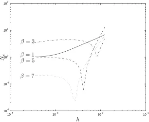
1D fourth-order problem

This test problem is governed by

d4_u

dx4 +

d2_u

dx2 = exp(−5x) [98490650 sin(100x) + 19949000 cos(100x)], −1≤x≤1,

(46)

with Dirichlet boundary conditions

u(0) = 0, du

dx(0) = 100,

u(1) = sin(100) exp(−5), du

dx(1) = 100 cos(100) exp(−5)−5 sin(100) exp(−5),

for which the exact solution is also given in the form of (45). Four subdomains

are considered. Grid convergence is studied using various sets of collocation points,

namely (11,21,31,· · · ,701) points/subdomain. A test set of 201 uniformly

dis-tributed points is employed to compute the error Ne.

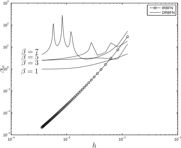
The continuity of the approximate solution at the interfaces is imposed up to

third-order derivative for MD-DRBFNs and fourth-third-order derivative for MD-IRBFNs.

Fig-ure 5 shows accuracy against grid refinement by the two multidomain RBF

tech-niques, indicating a superior performance of MD-IRBFNs over MD-DRBFNs.

lead to better accuracy, probably due to the effect of implementing multiple

bound-ary conditions. The ODE on each subdomain is collocated at (n−4) grid points for

MD-DRBFNs and n points for MD-IRBFNs. To investigate this issue separately,

we solve the above problem by the one-domain DRBFN method. The same grid

sizes are used. Two boundary points and two adjacent interior points are set to

implement the double boundary conditions. Results obtained are shown in Figure

6. For β = 1, the convergence behaviour is smooth, but its rate is very slow. For

higher values ofβ, the technique gives a fast rate of convergence over coarse grids. However, the accuracy of the solution then deteriorates rapidly over fine grids. It

can be seen that the grid-convergence behaviour of the one-domain DRBFN method

is not stable, which may cause a poor performance of the MD-DRBFN technique

here.

5.3

2D second-order problem

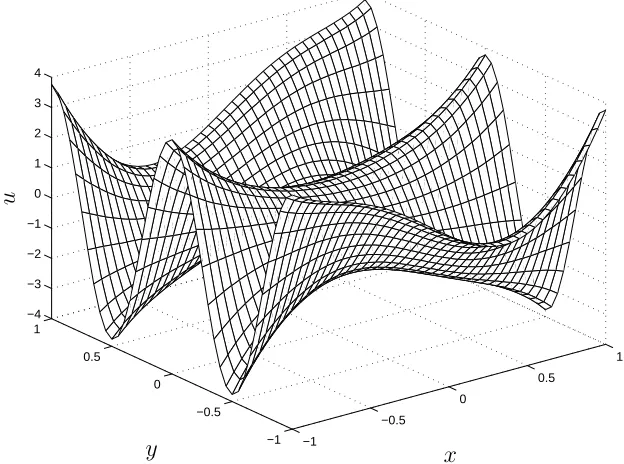
Consider the Poisson equation

∂2_u

∂x2 +

∂2_u

∂y2 = (1−π

2_{) sin(πx) sinh(y) + 4(1−π}2_{) cosh(2x) cos(2πy), (47)}

on the domain −1≤x, y ≤1, subject to Dirichlet boundary conditions

u= cosh(±2) cos(2πy), x=±1, and

u= sin(πx) sinh(±1) + cosh(2x), y=±1.

The exact solution of this problem is given by

Figure 7 shows the variation of (48) over the domain of interest. Only IRBFNs

are applied here to solve this problem. The relative L2 norm of the approximate

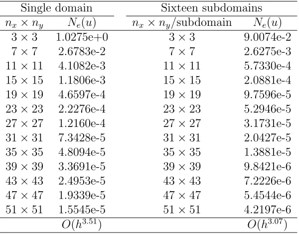
solution (Ne) is computed at the grid points. Results concerning Ne for two cases,

single domain and 16 subdomains, are presented in Table 2. Values of the condition

number of the IRBFN system matrix vary from 1.0e0 to 2.4e3 for grids of 3×3 to

51×51/subdomain, respectively. It can be seen that the MD-IRBFN technique is

able to employ much larger numbers of collocation points (e.g., up to 40,400 grid

points used here without suffering from the problem of ill-conditioned matrices).

The achievement of higher-order smoothness of the present DD solution across the

subdomain interfaces is expected to alleviate the deterioration in accuracy caused

by the domain division. Numerical results show that the convergence rate is reduced

fromO(h3.51_{) (single domain) toO(h}3.07_{) (16 subdomains). This amount of reduction}

appears to be relatively small. Owing to smaller grid sizes used, the MD-IRBFN

results are more accurate than the one-domain IRBFN results. Furthermore, the

MD-IRBFN method only needs to handle a set of smaller matrices (i.e. a matrix

for the unknowns on the interfaces and matrices for the interior values of the field

variable on subdomains), leading to an improvement in computational efficiency

over the one-domain IRBFN method.

5.4

2D fourth-order problem

This test problem is governed by the biharmonic equation with Dirichlet boundary

conditions (u and ∂u/∂n). The domain of interest is a square region of size 2×2

that is centered at the origin. The exact solution is chosen to be the same as that

of the previous problem, i.e. (48), from which one can easily derive expressions

for the forcing function b and the boundary conditions. The problem domain is

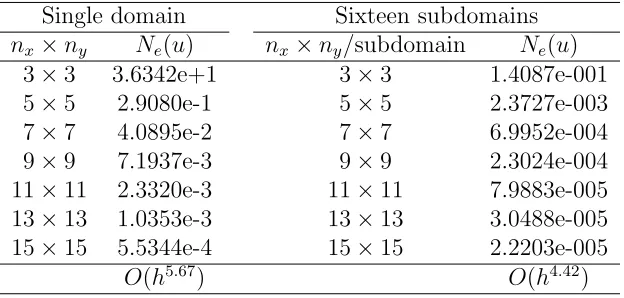
using a number of grids, namely 3×3, 5×5,· · · ,and 15×15. RelativeL2errors (Ne)

of the solutionuobtained by the one-domain and multidomain IRBFN methods are

presented in Table 3. Grid densities used for both methods are the same. The

size of MD-IRBFN matrices is thus comparable with that of one-domain IRBFN

matrices. However, the grid spacing of the former is 4 times smaller than that of

the latter. For grids employed here, the condition numbers of the IRBFN system

matrix are in the range of 1.0e0 to 4.5e4. As expected, the rate of convergence of

the MD-IRBFN solution is reduced relative to the case of single domain. However,

the DD method still yields a fast convergence rate up to O(h4.42_{), resulting in very}

accurate solutions (e.g. Ne(u)=2.2e-5 is obtained with a density of 15×15). Given

the same exact solution and the same number of subdomains, Tables 2 and 3 show

that the MD-IRBFN technique performs better for the fourth-order PDE than for

the second-order PDE.

6

Concluding remarks

In this paper, one-dimensional IRBFN interpolation schemes are incorporated into

the substructuring technique for the solution of second- and fourth-order elliptic

problems. The constants of integration in IRBFNs are exploited to improve the

continuity order of the approximate solution across the subdomain interfaces.

Addi-tional enforcements are applied at the intersection points, which allows the solution

at these points to be continuous across the subdomain interface with the same

order as that at the interface points. Numerical results show that the proposed

domain-decomposition technique yields a high level of accuracy and a fast rate of

convergence. The multidomain IRBFN method thus appears to be more attractive

Acknowledgement

This work is supported by the Australian Research Council. We would like to thank

the referees for their helpful comments.

References

1. B.F. Smith, P.E. Bjorstad and W.D. Gropp, Domain Decomposition

Paral-lel Multilevel Methods for Elliptic Partial Differential Equations, New York,

Cambridge University Press, 1996.

2. E.J. Kansa, Multiquadrics- A scattered data approximation scheme with

appli-cations to computational fluid-dynamics-II. Solutions to parabolic, hyperbolic

and elliptic partial differential equations, Computers and Mathematics with

Applications 19(8/9) (1990), 147–161.

3. G.E. Fasshauer, “Solving partial differential equations by collocation with

ra-dial basis functions”, A. LeMhaut, C. Rabut and L.L. Schumaker, editors,

Surface Fitting and Multiresolution Methods, Vanderbilt University Press,

Nashville, TN, 1997, pp. 131–138.

4. M.R. Dubal, Domain decomposition and local refinement for multiquadric

ap-proximations. I: Second-order equations in one-dimension, Journal of Applied

Science and Computation 1(1) (1994), 146–171.

5. E.J. Kansa and Y.C. Hon, Circumventing the ill-conditioning problem with

multiquadric radial basis functions: applications to elliptic partial differential

equations, Computers and Mathematics with Applications 39 (2000), 123–137.

6. J. Li and Y.C. Hon, Domain decomposition for radial basis meshless methods,

7. M.S. Ingber, C.S. Chen and J.A. Tanski, A mesh free approach using radial

ba-sis functions and parallel domain decomposition for solving three-dimensional

diffusion equations, International Journal for Numerical Methods in

Engineer-ing 60(13) (2004), 2183-2201.

8. E. Divo and A. Kassab, Iterative domain decomposition meshless method

mod-eling of incompressible viscous flows and conjugate heat transfer, Engineering

Analysis with Boundary Elements 30(6) (2006), 465–478.

9. C.K. Lee, X. Liu and S.C. Fan, Local multiquadric approximation for solving

boundary value problems, Computational Mechanics 30(5–6) (2003), 396–409.

10. C. Shu, H. Ding and K.S. Yeo, Local radial basis function-based differential

quadrature method and its application to solve two-dimensional

incompress-ible Navier-Stokes equations, Computer Methods in Applied Mechanics and

Engineering 192 (2003), 941–954.

11. B. Sarler and R. Vertnik, Meshfree explicit local radial basis function

colloca-tion method for diffusion problems, Computers & Mathematics with

Applica-tions 51(8) (2006), 1269–1282.

12. N. Mai-Duy and R.I. Tanner, A collocation method based on one-dimensional

RBF interpolation scheme for solving PDEs, International Journal of

Numer-ical Methods for Heat & Fluid Flow 17(2) (2007), 165-186.

13. N. Mai-Duy and T. Tran-Cong, A Cartesian-grid collocation method based on

radial-basis-function networks for solving PDEs in irregular domains,

Numer-ical Methods for Partial Differential Equations 23 (2007), 1192–1210.

14. N. Mai-Duy and T. Tran-Cong, Approximation of function and its

15. E.J. Kansa, H. Power, G.E. Fasshauer and L. Ling, A volumetric integral radial

basis function method for time-dependent partial differential equations: I.

Formulation, Engineering Analysis with Boundary Elements 28 (2004), 1191–

1206.

16. N. Mai-Duy and T. Tran-Cong, Numerical solution of differential equations

us-ing multiquadric radial basis function networks, Neural Networks 14(2) (2001),

185–199.

17. L. Ling and M.R. Trummer, Multiquadric collocation method with integral

formulation for boundary layer problems, Computers & Mathematics with

Applications 48(5–6) (2004), 927–941.

18. S.A. Sarra, Integrated multiquadric radial basis function approximation

meth-ods, Computers & Mathematics with Applications 51(8) (2006), 1283–1296.

19. N. Mai-Duy, Solving high order ordinary differential equations with radial

basis function networks, International Journal for Numerical Methods in

En-gineering 62 (2005), 824–852.

20. N. Mai-Duy and R.I. Tanner, Solving high order partial differential equations

with indirect radial basis function networks, International Journal for

Numer-ical Methods in Engineering 63 (2005), 1636–1654.

21. N. Mai-Duy and T. Tran-Cong, Solving biharmonic problems with

scattered-point discretisation using indirect radial-basis-function networks, Engineering

Table 1: 1D second-order problem, 2 subdomains, β = 1: Relative L2 errors and

their orders by the MD-DRBFN and MD-IRBFN methods

n/subdomain MD-DRBFNs MD-IRBFNs

11 1.8993e+1 2.2079e+1

21 1.7530e+0 2.7877e-1

31 1.1146e+0 7.3596e-2

41 8.3960e-1 3.4584e-2

51 6.7971e-1 1.8495e-2

61 5.7443e-1 1.0932e-2

71 4.9945e-1 6.9591e-3

81 4.4310e-1 4.6839e-3

91 3.9907e-1 3.2914e-3

101 3.6363e-1 2.3938e-3

111 3.3448e-1 1.7907e-3

121 3.1002e-1 1.3710e-3

131 2.8919e-1 1.0703e-3

141 2.7123e-1 8.4952e-4

151 2.5558e-1 6.8402e-4

161 2.4181e-1 5.5768e-4

171 2.2959e-1 4.5973e-4

181 2.1868e-1 3.8272e-4

191 2.0888e-1 3.2143e-4

201 2.0001e-1 2.7206e-4

Table 2: 2D second-order problem: RelativeL2 errors and their orders by the

one-domain and multione-domain IRBFN methods

Single domain Sixteen subdomains

nx×ny Ne(u) nx×ny/subdomain Ne(u)

3×3 1.0275e+0 3×3 9.0074e-2

7×7 2.6783e-2 7×7 2.6275e-3

11×11 4.1082e-3 11×11 5.7330e-4

15×15 1.1806e-3 15×15 2.0881e-4

19×19 4.6597e-4 19×19 9.7596e-5

23×23 2.2276e-4 23×23 5.2946e-5

27×27 1.2160e-4 27×27 3.1731e-5

31×31 7.3428e-5 31×31 2.0427e-5

35×35 4.8094e-5 35×35 1.3881e-5

39×39 3.3691e-5 39×39 9.8421e-6

43×43 2.4953e-5 43×43 7.2226e-6

47×47 1.9339e-5 47×47 5.4544e-6

51×51 1.5545e-5 51×51 4.2197e-6

Table 3: 2D fourth-order problem: Relative L2 errors and their orders by the

one-domain and multione-domain IRBFN methods

Single domain Sixteen subdomains

nx×ny Ne(u) nx×ny/subdomain Ne(u)

3×3 3.6342e+1 3×3 1.4087e-001

5×5 2.9080e-1 5×5 2.3727e-003

7×7 4.0895e-2 7×7 6.9952e-004

9×9 7.1937e-3 9×9 2.3024e-004

11×11 2.3320e-3 11×11 7.9883e-005

13×13 1.0353e-3 13×13 3.0488e-005

15×15 5.5344e-4 15×15 2.2203e-005

0 0.1 0.2 0.3 0.4 0.5 0.6 0.7 0.8 0.9 1 −0.8

−0.6 −0.4 −0.2 0 0.2 0.4 0.6 0.8 1

x

u

10−3 10−2 10−1

10−4

10−3

10−2

10−1

100

101

102

103

104

IRBFN DRBFN

h

Ne

β = 1

β = 3

β = 5

β = 7

β = 9

β = 11

Figure 3: 1D second-order problem, 2 subdomains: ErrorNeversus the grid spacing

0 0.1 0.2 0.3 0.4 0.5 0.6 0.7 0.8 0.9 1

10−12

10−11

10−10

10−9

10−8

10−7

10−6

10−5

10−4

10−3

x

|

u

−

ue

|

10−4 10−3 10−2 10−1

10−3

10−2

10−1

100

101

102

103

IRBFN DRBFN

h

Ne β = 1

β = 3

ββ= 5= 7

Figure 5: 1D fourth-order problem, 4 subdomains: ErrorNe versus the grid spacing

10−4 10−3 10−2 10−1

10−2

10−1

100

101

102

h

Ne β = 1

β = 3

β = 5

β = 7

Figure 6: 1D fourth-order problem: Error Ne versus the grid spacing h by the

−1

−0.5 0

0.5

1

−1 −0.5 0 0.5 1 −4 −3 −2 −1 0 1 2 3 4

x y

u