A Cartesian-grid discretisation scheme based on local integrated RBFNs for two-dimensional elliptic problems

A Cartesian-grid discretisation scheme based on local integrated RBFNs for two-dimensional elliptic problems

N. Mai-Duy, CESRC, Faculty of Engineering & Surveying, USQ, Australia T. Tran-Cong, CESRC, Faculty of Engineering & Surveying, USQ, Australia.

Abstract: This paper reports a new numerical scheme based on Cartesian grids and local in-tegrated radial-basis-function networks (IRBFNs) for the solution of second-order elliptic dif-ferential problems defined on two-dimensional regular and irregular domains. At each grid point, only neighbouring nodes are activated to construct the IRBFN approximations. Local IRBFNs are introduced into two different schemes for discretisation of partial differential equa-tions, namely point collocation and control-volume (CV)/subregion-collocation. Linear (e.g. heat flow) and nonlinear (e.g. lid-driven triangular-cavity fluid flow) problems are considered. Numerical results indicate that the local IRBFN CV scheme outperforms the local IRBFN point-collocation scheme regarding accuracy. Moreover, the former shows a similar level of the matrix condition number and a significant improvement in accuracy over a linear CV method.

Keyword: local approximations, integrated RBFNs, point collocation, subregion collocation, second-order differential problems.

1 Introduction

RBF-based discretisation methods have emerged as a new attractive solver for partial differential equations (PDEs) (e.g. [Fasshauer (2007)]). They have the capability to work well for problems defined on irregular domains. Very accurate results can be achieved using only a relatively-small number of nodes. However, RBF matrices are dense and generally ill-conditioned. To resolve this problem, local RBF methods have been developed, resulting in having to solve a sparse system of algebraic equations. The RBF approximations are constructed locally on small overlapping regions which are represented by a set of structured points or a set of scattered points. Works reported include [Lee, Liu, and Fan (2003); Shu, Ding, and Yeo (2003); Tol-stykh and Shirobokov (2003); Chantasiriwan (2004); Shu, Ding, and Yeo (2005); TolTol-stykh and Shirobokov (2005); Wright and Fornberg (2006); Kosec and Sarler (2008a); Kosec and Sarler (2008b); Orsini, Power, and Morvan (2008); Sanyasiraju and Chandhini (2008); Vertnik and Sarler (2009)].

Cartesian grids to represent the domain is economical. Considerable effort has been put into the development of Cartesian-grid-based computational techniques (e.g. [Johansen and Colella (1998); Jomaa and Macaskill (2005); Hu, Young, and Fan (2008); Parussini and Pediroda (2008); Pasquim and Mariani (2008); Bourantas, Skouras, and Nikiforidis (2009)]).

The proposed numerical procedure combines strengths of the local RBF approach and the Cartesian-grid approach for solving 2D differential problems. At each Cartesian-grid point, only neighbouring nodes are activated to construct the RBF approximations. Unlike local RBF techniques reported in the literature, RBFNs are employed here to approximate highest-order derivatives in a given PDE and subsequently integrated to obtain expressions for lower-order derivatives and the field vari-able [Mai-Duy and Tran-Cong (2001)]. This use of integration to construct the approximations provides an effective way to circumvent the problem of reduced convergence rate caused by differentiation and to implement derivative boundary conditions (e.g. [Duy (2005); Mai-Duy and Tran-Cong (2006)]). In this study, we introduce local integrated RBFNs into two PDE discretisation formulations, namely point collocation and control-volume (CV)/subregion-collocation, and then conduct some numerical experiments to investigate accuracy of the two local IRBFN techniques.

Recirculating viscous flows in enclosed cavities have received a great deal of attention in fluid mechanics community as they can produce interesting flow features at different Reynolds num-bers. Examples of this type include lid-driven flows in square and triangular cavities. For such problems, at the two top corners, the velocity is discontinuous and the stress is unbounded. These pose great challenges for numerical simulation. In contrast to the square cavity problem, the triangular cavity flow presents a severe test for structured-grid-based numerical methods (e.g. [Jyotsna and Vanka (1995)]). The latter is chosen here to investigate the performance of the present local IRBFN CV technique. The flow is simulated using the streamfunction and vor-ticity formulation discretised on rectangular grids. Attractive features of the proposed technique are (i) no coordinate transformations are required and (ii) computational boundary conditions for the vorticity are derived in a new effective way, where analytic formulae that need only nodal values of the streamfuntion on one grid line [Le-Cao, Mai-Duy, and Tran-Cong (2009)] are utilised.

The remainder of this paper is organised as follows. A brief review of integrated RBFNs is given in Section 2. The proposed computational procedure is presented in Section 3 and numerically verified through a series of examples in Section 4. Section 5 concludes the paper.

2 Integrated radial-basis-function networks

RBFNs allow a conversion of a function f from a low-dimensional space (e.g. 1D-3D) to a high-dimensional space in which the function can be expressed as a linear combination of RBFs

f(x) =

m

∑

i=1

where the superscript (i) is the summation index, x the input vector, m the number of RBFs, {w(i)}m

i=1the set of network weights to be found, and{G(i)(x)}mi=1the set of RBFs.

This study is concerned with second-order differential problems in two dimensions. The inte-gral approach [Mai-Duy and Tran-Cong (2001)] uses RBFNs (1) to represent the second-order derivatives of the field variable u in a given PDE. Approximate expressions for the first-order derivatives and the variable itself are then obtained through integration as

∂2_u(x)

∂x2_j = m

∑

i=1

w(_[xji)_]G(i)(x), (2)

∂u(x)

∂xj

=

m

∑

i=1

w(_[xji)_]H_[(_xji)_](x) +C1[xj](xk), (3)

u[xj](x) = m

∑

i=1

w(_[xji)_]H(_[xi)

j](x) +xjC1[xj](xk) +C2[xj](xk), (4) where the subscript[xj]is used to denote the quantities associated with the process of integration with respect to the xj variable; C1[xj](xk) and C2[xj](xk) the constants of integration which are

univariate functions of the variable other than xj(i.e. xkwith k6= j); H_[(_xji)_](x) =RG(i)(x)dxjand H(_[xi)

j](x) =

R

H_[(_xji)_](x)dxj. The reader is referred to [Mai-Duy and Tran-Cong (2001); Mai-Duy and Tanner (2005); Mai-Duy (2005);Mai-Duy and Tran-Cong (2005)] for further details (e.g. explicit forms of integrated and differentiated RBFs).

3 Proposed technique

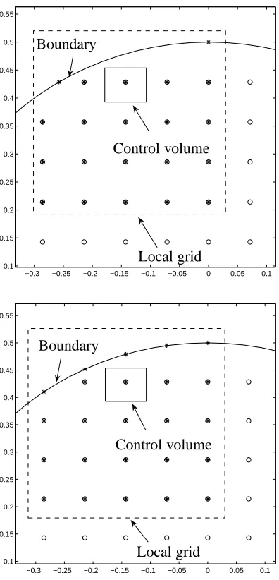
The 2D problem domain is discretised using a Cartesian grid. Boundary points are generated through the intersection of the grid lines and the boundaries. For a reference point, we form two local integrated networks using (2)-(4): one associated with the x1coordinate and the other with

the x2 coordinate. The two networks are constructed on the same set of l×l grid lines. The

reference point may not be the centre of the local grid when the construction process is carried out near the boundary (Figure 1).

For local grids entirely embedded in the domain, the two networks have the same set of RBF centres which are chosen to be the interior grid nodes. The value of m in (4) is equal to l2. For local grids that are cut by irregular boundary, one generally has different sets of RBF centres for the two associated networks. A set of the RBF centres for the xjnetwork is comprised of the interior grid nodes and the boundary nodes generated by the xj grid lines. The value of m in (4) may be less than l2(Figure 1).

subscripts_1[xj]and_2[xj]are dropped. The function C(xk)is constructed through d2C(xk)

dx2_k = l

∑

i=1

w(i)g(i)(xk), (5)

dC(xk)

dxk

=

l

∑

i=1

w(i)h(i)(xk) +c1, (6)

C(xk) =

l

∑

i=1

w(i)¯h(i)(xk) +xkc1+c2, (7)

where c1and c2are the constants of integration which are simply unknown values, and g(i), h(i)

and ¯h(i) the one-dimensional forms of G(i), H(i) and H(i), respectively. Collocating (7) at the local grid points x(_ki)with i=_{1,2,_···,l_}leads to

b

C=Tc_{wb, (8)}

whereC andb w are the vectors of length l and_b (l+2), respectively, andTc_{is the transformation}

matrix of dimensions l_×(l+2)

b

C=C(x(_k1)),C(x(_k2)),_···,C(x(_kl))T=C(1),C(2),_···,C(l) T

,

b

w=w(1),w(2),_···,w(l),c1,c2

T , c T ₌      

¯h(1)_(x(1)

k ), ¯h(2)(x

(1)

k ), ···, ¯h(l)(x

(1)

k ), x

(1)

k , 1 ¯h(1)_(x(2)

k ), ¯h(2)(x

(2)

k ), ···, ¯h(l)(x

(2)

k ), x

(2)

k , 1 ..

. ... . .. ... ... ...

¯h(1)_(x(l)

k ), ¯h(2)(x

(l)

k ), ···, ¯h(l)(x

(l)

k ), x

(l)

k , 1      .

Taking (8) into account, the value of C in (7) at an arbitrary point xk can be computed in terms of nodal values of C as

C(xk) =h¯h(1)_(xk),¯h(2)_{(xk),···,¯h}(l)_(xk),xk,1i_Tc+_{Cb, (9)}

or C(xk) =

l

∑

i=1

P(i)(xk)C(i), (10)

where P(i)(xk)is the product of the first vector on RHS and the ith column ofTc+, andTc+ is the generalised inverse ofTc_{of dimensions(l+2)×l, which can be obtained using the SVD}

Substitution of (10) into (3) and (4) yields ∂u(x)

∂xj

=

m

∑

i=1

w_[(_xji)_]H_[(_xji)_](x) +

l

∑

i=1

P_[(_xji)_](xk)C(₁i_[)_xj], (11)

u[xj](x) = m

∑

i=1

w(_[xji)_]H(_[xi) j](x) +

l

∑

i=1

xjP_[(_xji)_](xk)C(₁i_[)_xj]+

l

∑

i=1

P_[(_xi) j](xk)C

(i)

2[xj]. (12)

For convenience of presentation, expressions (2), (11) and (12) can be rewritten as ∂2_u(x)

∂x2_j = m+2l

∑

i=1

w(_[xji)_]G(_[xi)

j](x), (13)

∂u(x)

∂xj

=

m+2l

∑

i=1

w_[(_xji)_]H_[(_xji)_](x), (14)

u_[xj](x) =

m+2l

∑

i=1

w(_[xji)_]H(_[xi)

j](x), (15)

where {G(_[xi)

j](x)} m+2l

i=m+1≡ {0}2li=1,

{H_[(_xji)_](x)_}m_i=+_ml_{+1≡ {}P_[(_xji)_](xk)_}l_i=1, _{H_[(_xi) j](x)}

m+2l

i=m+l+1≡ {0}

l i=1,

{H(_[xi) j](x)}

m+l

i=m+1≡ {xjP_[(_xji)_](xk)}li=1, {H (i)

[xj](x)}mi=+m2l+l+1≡ {P (i) [xj](xk)}

l i=1,

{w(_[xi) j]}

m+l

i=m+1≡ {C (i) 1[xj]}

l

i=1,and{w (i) [xj]}

m+2l

i=m+l+1≡ {C (i) 2[xj]}

l i=1.

We seek the solution in terms of nodal values of the field variable u. To do so, (15) is collocated at the nodal points on the local grid, from which the relationship between the network-weight space and the physical space can be established as

e

u[xj] = Tf[xj]we[xj], (16)

e

w_[xj] = Tf+

[xj]ue[xj], (17)

whereue[xj] is the vector of length m consisting of the nodal values of u on the local grid,we[xj] the vector of length (m+2l) made up of the RBF weights and the nodal values of C₁(i_[)_xj] and C(₂i_[)_xj], andTf+

[xj] the generalised inverse ofTf[xj]. The transformation matrixTf[xj]has the entries

f

T_[x

j]rs=H

(s) [xj](x

(r)_{), where 1≤r≤m and 1≤s≤(m+2l).}

It is noted that the two vectors,u_e[x1]andue[x2], are unknown. From now on, they are forced to be

identical e

The values of u,∂u/∂xjand∂2u/∂x2j at an arbitrary point x can be computed in terms of nodal variable values as

u(x) =1

2

2

∑

j=1

u_[xj](x) =1

2

2

∑

j=1

h

H_[(_xj1)_](x),H_[(_xj2)_](x),_···,H(_[xm+2l) j] (x)

i f

T+

[xj]

e

u, (19)

∂u(x)

∂xj

=hH_[(_xj1)_](x),H_[(_xj2)_](x),_···,H_[(_xm+2l) j] (x)

i f

T+

[xj]eu, (20)

∂2_u(x)

∂x2_j = h

G(1)(x),G(2)(x),_···,G(m+2l)(x)iTf+

[xj]ue. (21)

In (19), there are two integrated networks in the x1and x2directions that produce two values of

the function at a point. Theoretically, they are the same. However, due to approximation errors, these two values are not identical. As a result, the function value is computed by taking the average of the two.

For the point-collocation formulation, there are no integrations required for the discretisation. The process of converting the PDE into a set of algebraic equations is straightforward.

For the control-volume formulation, one has to define a control volume for each node, over which the PDE will be integrated. The control volume is formed using the lines that are parallel to the x1 and x2 axes and go through the middle points between the reference node and its

neighbours or appropriate points on the boundary (Figure 1). Integrals can be calculated using high-order (e.g. 5-points used here) Gauss quadrature since the present approximation scheme allows the accurate evaluation of the variable u and its derivatives at any point within the local grid.

The use of local integrated networks results in a sparse system of simultaneous equations. It can be seen that operations on zero elements are unnecessary. Avoiding these operations provides a considerable saving in time. By taking account of sparseness of the system matrix, one has the capability to reduce the computational time and storage facilities. Such sparse equation sets can be solved effectively by means of iterative solvers (e.g. generalised minimum residual methods). 4 Numerical examples

For all numerical examples presented here, the approximations are constructed on local grids of 5_×5. IRBFNs are implemented with the multiquadric (MQ) basis function whose form is given G(i)(x) =

q

(x₋c(i)₎T_(x−c(i)_{) +a}(i)2_{, (22)}

determine the optimal value of the shape parameter in practice. In this study, we do not focus on the study of the RBF width. All MQ centres are associated with the same width that is chosen to be the grid size. For problems whose exact solution is available, we use the discrete relative L2 norm of u, denoted by Ne(u), to measure accuracy of an approximate scheme. We apply

the matrix 1-norm estimation algorithm for estimating condition numbers of the system matrix. Furthermore, linear CV (central difference) techniques, which are similar to those described in [Patankar (1980)], are referred to as a standard CV technique.

4.1 Test problem

Consider the following PDE ∂2_u

∂x2₁ + ∂2_u

∂x2₂ =0 (23)

with Dirichlet boundary conditions. Two computational domains, namely a unit square 0_≤ x1,x2≤1 and a circle centered at the origin with radius of 0.5, are considered. The exact

solution is given by ue= 1

sinh(π)sin(πx1)sinh(πx2) (24)

from which the boundary values of u can be derived.

The point-collocation formulation consists in forcing (23) to be satisfied exactly at discrete points in order to form a determined set of algebraic equations. It means that (23) needs be collocated at the interior grid nodes.

For the control-volume formulation, (23) is forced to be satisfied in the mean. Integrating (23) over a control volumeΩi, we have

Z

Ωi∇

2_{udΩi=0. (25)}

Using the divergence theorem, (25) becomes

Z

Γi(∇u·n)dΓi=0, (26)

whereΓi is the boundary ofΩi and n the outward normal unit vector. To compute∂u/∂xj on the faces that are parallel to the xk(k₆=j)direction, we use the xj network.

Uniform Cartesian grids are employed to represent the problem domain.

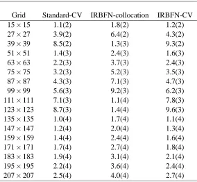
a similar level of the matrix condition number. The use of local approximations leads to a significant improvement in stability over that of global approximations. It was reported in the literature that the global RBF matrices may be ill-conditioned when using 1000 nodes. Here, with 42849 nodes taken, condition numbers of the RBF matrix are only O(104). In terms of accuracy, both RBF methods are more accurate than the standard CV method as shown in Figure 2. The IRBFN-CV method outperforms the IRBFN-collocation method. Given a grid size, the CPU time for the IRBFN-CVM solution is seen to be greater than that for the standard-CVM solution. However, from Figure 2, the IRBFN-CVM is much more accurate than the standard CVM. To achieve a similar level of accuracy, it is necessary to use denser grids for the standard CVM. For example, to yield Ne=1.9_×10−7, one needs to employ approximately a grid of 1701_×1701 for the standard CVM (this grid density is estimated through extrapolation) and only 203_×203 for the IRBFN CVM. It is noted that very high grid densities lead to ill-conditioned matrices. For a given accuracy, the IRBFN CVM can thus be more efficient than the standard CVM. Figure 3 shows the locations of nonzero entries in the IRBFN system matrix.

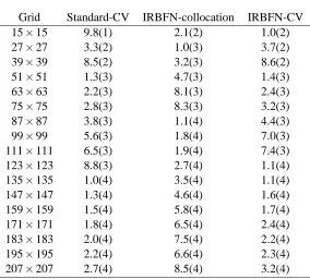
In the case of circular domain, we generate boundary nodes through the intersection of the grid lines and the boundary. It can be seen that there may be some interior grid nodes that are very close to the boundary. A parameter∆=h/8 is introduced here. Interior nodes, which fall within a small distance∆to the boundary, are set aside. The matrix condition number and the accuracy of the three methods are shown in Table 2 and Figure 4. Remarks for this case are similar to those for the rectangular case.

Theoretical studies [Sarra (2006)] showed that IRBFNs have higher approximation power than differentiated RBFNs. The implementation of local- and global-IRBFN versions incorporating Cartesian grids shares many common features. The latter was presented in detail in our previous works [Mai-Duy and Tran-Cong (2009a); Mai-Duy and Tran-Cong (2009b)]. For the handling of a Neumann boundary condition on a curved boundary, the reader is referred to [Mai-Duy and Tran-Cong (2009b)] for a full detail. Generally speaking, global versions are capable of giving more accurate results than local versions. However, global schemes produce fully-populated matrices that may limit the number of nodes to a few hundreds only. For problems, which require a relatively-dense discretisation for an accurate simulation, the use of local schemes is a preferred option.

Numerical experiments studied here indicate that the control volume formulation works better for local IRBFNs than the collocation formulation. The IRBFN-CV method is now applied to simulate some heat transfer and fluid flow problems.

4.2 Heat flow

Find the temperatureθ such that ∇.

vθ₋ 1

Pe∇θ

where v is a prescribed velocity,Ωthe domain and Pe the Peclet number. Here,Ωand v are taken as[0,1]_×[₋0.5,0.5]and(1,0)T_{, respectively. Boundary conditions are prescribed as follows}

θ=0, for x2=−0.5 and x2=0.5, (28)

θ=cos(πx2) for x1=0, and (29)

θ=0 for x1=1. (30)

The exact solution to this problem can be verified to be θe= cos(πx2)

exp(a)₋exp(b)(exp(a+bx1)−exp(b+ax1)), (31)

where a=0.5Pe+√Pe2₊₄π2_{and b=0.5Pe−}√_Pe2₊₄π2_{. This problem is taken from}

[Kohno and Bathe (2006)].

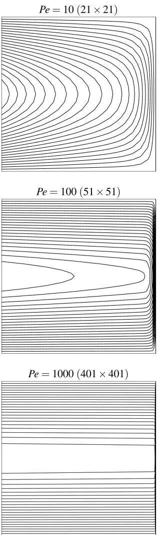
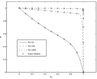
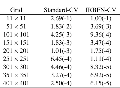
The temperature boundary layer becomes thinner with increasing Pe. At Pe=1000, very steep boundary layer is formed. Figure 5 shows the temperature contours for three different values of Pe by the present CV method. Its accuracy is better than that of the standard CV method as shown in Table 3. Figure 6 displays variations of temperature along the centre line. It can be seen that the proposed method produces very accurate results for all cases. Figure 7 show that there are no fluctuations in the IRBFN CVM solution.

4.3 Lid-driven triangular-cavity flow

Consider the steady recirculating flow of a Newtonian fluid in an equilateral triangular cavity. Figure 8 shows the cavity geometry. We take P=√3 and Q=3. The lid moves from left to right with a unit velocity (v= (1,0)T_{), while the left and right walls are stationary (v= (0,0)}T_{). The} problem was numerically studied by different techniques, including the finite-different method with a transformed geometry (e.g. [Ribbens, Watson, and Wang (1994)] and the finite-element method with a flow-condition-based interpolation (e.g. [Kohno and Bathe (2006)]).

Governing equations:

The governing equations are obtained from the streamfunction-vorticity formulation

ω=∇2ψ, (32)

∂ω ∂t +

v1_∂∂ω

x1

+v2_∂∂ω

x2

= 1

Re∇

2_{ω, (33)}

where Re is the Reynolds number defined as Re=U L/ν (L: the characteristic length, U : the characteristic velocity and ν the kinematic viscosity), ψ the streamfunction, ω the vorticity, v1=∂ψ/∂x2 and v2=−∂ψ/∂x1. The reference length and velocity are presently chosen as

Spatial discretisation:

The equilateral triangular cavity is discretised using a Cartesian grid. Grid nodes inside the cavity are taken to be the interior grid points. For this particular geometry, boundary nodes are generated using only grid lines that contain at least one interior grid node. With this approach, the set of RBF centres/collocation-points do not include the two top corners and hence infinite values of the vorticity do not enter the discrete system.

Boundary conditions:

Boundary conditions for the velocity lead toψ =0 and∂ψ/∂x2=1 on the lid, andψ=0 and

∂ψ/∂n=0 on the remaining walls (n: the direction normal to the wall).

We will use the boundary valuesψ =0 for solving the streamfunction equation. Fromψ =0 and ∂ψ/∂n=0, one obtains ∂ψ/∂x1 =0 and ∂ψ/∂x2=0 along the boundaries, which are

used for solving the vorticity equation. A vorticity boundary condition is computed through ωb=∂

2ψb

∂x2₁ + ∂2ψb

∂x2₂ , (34)

where the subscript b is used to indicate the boundary value. On the top wall, (34) reduces to ωb=∂

2_ψb

∂x2₂ . (35)

On the side walls, there are two possible cases

(i) A boundary point is also a grid node and the number of nodal points on the two associated grid lines are sufficiently-large for an accurate approximation, and

(ii) A boundary point is not a grid node or the number of nodal points on one of the two associ-ated grid lines is too small.

To computeωb, one can use (34) directly for the first case but may need to derive a suitable formula from (34), which requires information about ψ on one grid line only, for the second case. The latter will be handled here by applying formulae reported in our previous work (e.g. [Le-Cao, Mai-Duy, and Tran-Cong (2009)]), namely

ωb=

1+

t1

t2

_∂2ψb

∂x2₁ , (36)

for a x1-grid line, and

ωb=

1+

t2

t1

_∂2ψb

∂x2₂ , (37)

for a x2-grid line. In (36) and (37), t1 and t2are the x1- and x2-components of the unit vector

As mentioned earlier, one has to incorporate∂ψb/∂x1=0 and∂ψb/∂x2=0 into (35), (34), (36)

and (37). The incorporation process is similar to that in [Ho-Minh, Mai-Duy, and Tran-Cong (2009)]. It will be briefly reproduced here for the sake of completeness. Consider a xj grid line. On the line, one has

∂2ψ_(x)

∂x2

j

=

nj

∑

i=1

w(i)g(i)(xj) +0c1+0c2, (38)

∂ψ(xj) ∂xj

=

nj

∑

i=1

w(i)h(i)(xj) +c1+0c2, (39)

ψ(xj) = nj

∑

i=1

w(i)¯h(i)(xj) +xjc1+c2, (40)

where nj is the number of nodal points on the line and other notations are defined as before. There are two extra coefficients c1 and c2in (40). As a result, two extra equations representing

boundary derivative values∂ψ(x(_j1))/∂xjand∂ψ(x(_jnj))/∂xj can be added to the transformation system      b ψ

∂ψ(x(_j1)) ∂xj

∂ψ(x(jn j))

∂xj    

=Tcwb (41)

whereψb is the vector of nodal variable values of length nj, w the coefficient vector of lengthb

(nj+2)andTcis the transformation matrix of dimensions(nj+2)×(nj+2)

b

ψ =ψ(x(_j1)),ψ(x(_j2)),_···,ψ(x(_jnj))T, (42)

b

w=w(1),w(2),_···,w(nj),c1,c2

T , (43) c T ₌           

¯h(1)_(x(1)

j ), ¯h(2)(x

(1)

j ), ···, ¯h(nj)(x

(1)

j ), x

(1)

j , 1 ¯h(1)_(x(2)

j ), ¯h(2)(x

(2)

j ), ···, ¯h(nj)(x

(2)

j ), x

(2)

j , 1 ..

. ... . .. ... ... ...

¯h(1)_(x(nj)

j ), ¯h(2)(x

(nj)

j ), ···, ¯h(nj)(x

(nj)

j ), x

(nj)

j , 1 h(1)(x(_j1)), h(2)(x(_j1)), _···, h(nj)(x(_j1)), 1, 0 h(1)(x(_jnj)), h(2)(x(_jnj)), _···, h(nj)_(x(nj)

The values of∂2ψ/∂x2_j at the two boundary points can be computed by 

 

∂2_ψ(x(1)

j )

∂x2 j

∂2_ψ(x(n j) j )

∂x2 j

 

= (44)

"

g(1)(x(_j1)), g(2)(x(_j1)), _···, g(nj)_(x(1)

j ), 0, 0 g(1)(x(_jnj)), g(2)(x(_jnj)), _···, g(nj)(x(nj)

j ), 0, 0 #

c

T−1

     b ψ

∂ψ(x(_j1)) ∂xj

∂ψ(x(jn j))

∂xj    

, (45)

whereTc−1_{is an inverse of}Tc_.

By means of point collocation and integration constants, derivative boundary values are forced to be satisfied exactly. Moreover, all grid points on the associated grid lines are used to compute ωb. The present boundary schemes thus have a global property.

Four Cartesian grids, namely Grid 1 (2352 interior points), Grid 2 (5402 points), Grid 3 (9702 points) and Grid 4 (15252 points), are employed to study the convergence of the solution. The flow is simulated at the Reynolds number of 0, 100, 200 and 500. A time-marching approach is applied here to solve the present system of non-linear equations. For the vorticity transport equation (33), the diffusive and convective terms are treated implicitly and explicitly, respec-tively. We choose the initial solution to be the solution at a lower Re. For the case of Re=0, the flow starts from rest.

Figures 9 and 10 present contour plots of the streamfunction and vorticity variables, which look reasonable when compared with those available in the literature (e.g. [Ribbens, Watson, and Wang (1994); Kohno and Bathe (2006)]).

Figure 11 presents variations of the x1component of the velocity vector on the vertical centreline

x1 =0 and the x2 component of velocity on the horizontal line x2 =2. Results obtained by

[Kohno and Bathe (2006)] are also included for comparison purposes. It can be seen that the present results agree well with those by the flow-conditioned-based interpolation FEM for all values of Re.

5 Concluding remarks

control-volume technique has the capability to produce accurate results for the simulation of flow problems having steep gradients and complex patterns.

Acknowledgement: This work is supported by the Australian Research Council. We would like to thank the referees for their helpful comments.

References

Bourantas, G. C.; Skouras, E. D.; Nikiforidis, G. C. (2009): Adaptive support domain implementation on the moving least squares approximation for mfree methods applied on elliptic and parabolic pde problems using strong-form description. CMES: Computer Modeling in Engineering & Sciences, vol. 43, no. 1, pp. 1–26.

Chantasiriwan, S. (2004): Investigation of the use of radial basis functions in local colloca-tion method for solving diffusion problems. Internacolloca-tional Communicacolloca-tions in Heat and Mass Transfer, vol. 31, no. 8, pp. 1095–1104.

Fasshauer, G. E. (2007): Meshfree Approximation Methods With Matlab (Interdisciplinary Mathematical Sciences - Vol. 6). World Scientific Publishers.

Ho-Minh, D.; Mai-Duy, N.; Tran-Cong, T. (2009): A Galerkin-RBF approach for the streamfunction-vorticity-temperature formulation of natural convection in 2D enclosured do-mains. CMES: Computer Modeling in Engineering & Sciences, vol. 44, pp. 219–248.

Hu, S. P.; Young, D. L.; Fan, C. M. (2008): FDMFS for diffusion equation with unsteady forcing function. CMES: Computer Modeling in Engineering & Sciences, vol. 24, no. 1, pp. 1–20.

Johansen, H.; Colella, P. (1998): A Cartesian grid embedded boundary method for Poisson’s equation on irregular domains. Journal of Computational Physics, vol. 147, no. 1, pp. 60–85. Jomaa, Z.; Macaskill, C. (2005): The embedded finite difference method for the Poisson equation in a domain with an irregular boundary and Dirichlet boundary conditions. Journal of Computational Physics, vol. 202, no. 2, pp. 488–506.

Jyotsna, R.; Vanka, S. P. (1995): Multigrid calculation of steady, viscous flow in a triangular cavity. Journal of Computational Physics, vol. 122, no. 1, pp. 107–117.

Kosec, G.; Sarler, B. (2008a): Solution of thermo-fluid problems by collocation with local pressure correction. International Journal of Numerical Methods for Heat & Fluid Flow, vol. 18, pp. 868–882.

Kosec, G.; Sarler, B. (2008b): Local RBF Collocation Method for Darcy Flow. CMES: Computer Modeling in Engineering & Sciences, vol. 25, pp. 197–208.

Le-Cao, K.; Mai-Duy, N.; Tran-Cong, T. (2009): An effective integrated-RBFN Cartesian-grid discretisation for the stream function-vorticity-temperature formulation in non-rectangular domains. Numerical Heat Transfer, Part B, vol. 55, pp. 480–502.

Lee, C. K.; Liu, X.; Fan, S. C. (2003): Local multiquadric approximation for solving boundary value problems. Computational Mechanics, vol. 30, no. 5-6, pp. 396–409.

Mai-Duy, N. (2005): Solving high order ordinary differential equations with radial basis function networks. International Journal for Numerical Methods in Engineering, vol. 62, pp. 824–852.

Mai-Duy, N.; Tanner, R. I. (2005): An effective high order interpolation scheme in BIEM for biharmonic boundary value problems. Engineering Analysis with Boundary Elements, vol. 29, pp. 210–223.

Mai-Duy, N.; Tran-Cong, T. (2001): Numerical solution of differential equations using mul-tiquadric radial basis function networks. Neural Networks, vol. 14, no. 2, pp. 185–199.

Mai-Duy, N.; Tran-Cong, T. (2005): An efficient indirect RBFN-based method for numerical solution of PDEs. Numerical Methods for Partial Differential Equations, vol. 21, pp. 770–790. Mai-Duy, N.; Tran-Cong, T. (2006): Solving biharmonic problems with scattered-point dis-cretisation using indirect radial-basis-function networks. Engineering Analysis with Boundary Elements, vol. 30, no. 2, pp. 77–87.

Mai-Duy, N.; Tran-Cong, T. (2009a): A control volume technique based on integrated RBFNs for the convection-diffusion equation. Numerical Methods for Partial Differential Equations (accepted).

Mai-Duy, N.; Tran-Cong, T. (2009b): A numerical study of 2D integrated RBFNs incorporat-ing Cartesian grids for solvincorporat-ing 2D elliptic differential problems. Numerical Methods for Partial Differential Equations(accepted).

Parussini, L.; Pediroda, V. (2008): Investigation of multi geometric uncertainties by different polynomial chaos methodologies using a fictitious domain solver. CMES: Computer Modeling in Engineering & Sciences, vol. 23, no. 1, pp. 29–52.

Pasquim, B. M.; Mariani, V. C. (2008): Solutions for incompressible viscous flow in a triangular cavity using cartesian grid method. CMES: Computer Modeling in Engineering & Sciences, vol. 35, no. 2, pp. 113–132.

Patankar, S. V. (1980): Numerical Heat Transfer and Fluid Flow. McGraw-Hill.

Ribbens, C. J.; Watson, L. T.; Wang, C.-Y. (1994): Steady viscous flow in a triangular cavity. Journal of Computational Physics, vol. 112, no. 1, pp. 173–181.

Sanyasiraju, Y. V. S. S.; Chandhini, G. (2008): Local radial basis function based gridfree scheme for unsteady incompressible viscous flows. Journal of Computational Physics, vol. 227, no. 20, pp. 8922–8948.

Sarra, S. A. (2006): Integrated multiquadric radial basis function approximation methods. Computers & Mathematics with Applications, vol. 51, no. 8, pp. 1283–1296.

Shu, C.; Ding, H.; Yeo, K. S. (2003): Local radial basis function-based differential quadrature method and its application to solve two-dimensional incompressible Navier-Stokes equations. Computer Methods in Applied Mechanics and Engineering, vol. 192, pp. 941–954.

Shu, C.; Ding, H.; Yeo, K. S. (2005): Computation of incompressible navier-stokes equations by local RBF-based differential quadrature method. CMES: Computer Modeling in Engineering & Sciences, vol. 7, pp. 195–206.

Tolstykh, A. I.; Shirobokov, D. A. (2003): On using radial basis functions in a “finite differ-ence mode” with applications to elasticity problems. Computational Mechanics, vol. 33, no. 1, pp. 68–79.

Tolstykh, A. I.; Shirobokov, D. A. (2005): Using radial basis functions in a “finite difference mode”. CMES: Computer Modeling in Engineering & Sciences, vol. 7, pp. 207–222.

Vertnik, R.; Sarler, B. (2009): Solution of incompressible turbulent flow by a mesh-free method. CMES: Computer Modeling in Engineering & Sciences, vol. 44, pp. 65–96.

Table 1: Rectangular domain: Condition numbers of the system matrix by standard CV, local IRBFN collocation and local IRBFN CV methods. Notice that a(b)means a_×10b.

Grid Standard-CV IRBFN-collocation IRBFN-CV

15_×15 1.1(2) 1.8(2) 1.2(2)

27_×27 3.9(2) 6.4(2) 4.3(2)

39_×39 8.5(2) 1.3(3) 9.3(2)

51_×51 1.4(3) 2.4(3) 1.6(3)

63_×63 2.2(3) 3.7(3) 2.4(3)

75_×75 3.2(3) 5.2(3) 3.5(3)

87_×87 4.3(3) 7.1(3) 4.7(3)

99_×99 5.6(3) 9.2(3) 6.2(3)

111_×111 7.1(3) 1.1(4) 7.8(3)

123_×123 8.7(3) 1.4(4) 9.6(3)

135_×135 1.0(4) 1.7(4) 1.1(4)

147_×147 1.2(4) 2.0(4) 1.3(4)

159_×159 1.4(4) 2.4(4) 1.6(4)

171_×171 1.7(4) 2.7(4) 1.8(4)

183_×183 1.9(4) 3.1(4) 2.1(4)

195_×195 2.2(4) 3.6(4) 2.4(4)

Table 2: Circular domain: Condition numbers of the system matrix by standard CV, local IRBFN collocation and local IRBFN CV methods. Notice that a(b)means a_×10b.

Grid Standard-CV IRBFN-collocation IRBFN-CV

15_×15 9.8(1) 2.1(2) 1.0(2)

27_×27 3.3(2) 1.0(3) 3.7(2)

39_×39 8.5(2) 3.2(3) 8.6(2)

51_×51 1.3(3) 4.7(3) 1.4(3)

63_×63 2.2(3) 8.1(3) 2.4(3)

75_×75 2.8(3) 8.3(3) 3.2(3)

87_×87 3.8(3) 1.1(4) 4.4(3)

99_×99 5.6(3) 1.8(4) 7.0(3)

111_×111 6.5(3) 1.9(4) 7.4(3)

123_×123 8.8(3) 2.7(4) 1.1(4)

135_×135 1.0(4) 3.5(4) 1.1(4)

147_×147 1.3(4) 4.6(4) 1.6(4)

159_×159 1.5(4) 5.8(4) 1.7(4)

171_×171 1.8(4) 6.5(4) 2.4(4)

183_×183 2.0(4) 7.5(4) 2.2(4)

195_×195 2.2(4) 6.6(4) 2.3(4)

Table 3: Heat Flow, Pe=1000: Error Ne(u)by standard CV and local IRBFN CV methods. Notice that a(₋b)means a_×10−b.

Grid Standard-CV IRBFN-CV

11_×11 2.69(-1) 1.00(-1)

51_×51 1.83(-2) 3.69(-3)

−0.3 −0.25 −0.2 −0.15 −0.1 −0.05 0 0.05 0.1 0.1

0.15 0.2 0.25 0.3 0.35 0.4 0.45 0.5 0.55

Local grid Control volume Boundary

−0.3 −0.25 −0.2 −0.15 −0.1 −0.05 0 0.05 0.1 0.1

0.15 0.2 0.25 0.3 0.35 0.4 0.45 0.5 0.55

Local grid Control volume Boundary

10−3 10−2 10−1 100

10−7

10−6

10−5

10−4

10−3

10−2

10−1

Standard CVM IRBFN Collocation IRBFN CVM

h

N

e

(

u

)

0 0.5 1 1.5 2

x 104

0

0.5

1

1.5

2

x 104

nz = 549081

10−3 10−2 10−1 100

10−7

10−6

10−5

10−4

10−3

10−2

10−1

Standard CVM IRBFN Collocation IRBFN CVM

h

N

e

(

u

)

Pe=10(21_×21)

Pe=100(51_×51)

Pe=1000(401_×401)

0 0.2 0.4 0.6 0.8 1 0

0.2 0.4 0.6 0.8 1

Pe=10 Pe=100 Pe=1000 Exact solution

x1

u

0.96 0.98 1 1.02 1.04 1.06 0.7

0.75 0.8 0.85 0.9 0.95 1 1.05

1.1 _{Standard CVM}

IRBFN CVM

x1

u

x1

x2

(0,0)

(P,Q) (₋P,Q)

(ψ =0,∂ψ/∂n=0) (ψ=0,∂ψ/∂n=0)

(ψ=0,∂ψ/∂n=1)

Re=0, Grid 1 Re=100, Grid 2

Re=200, Grid 3 Re=500, Grid 4

Re=0, Grid 1 Re=100, Grid 2

Re=200, Grid 3 Re=500, Grid 4

−1.50 −1 −0.5 0 0.5 1 1.5 0.5

1 1.5 2 2.5 3

Grid 1

Grid 2

v₁ by FEM

v₂ by FEM

Re=100

−1.50 −1 −0.5 0 0.5 1 1.5

0.5 1 1.5 2 2.5 3

Grid 2

Grid 3

v₁ by FEM

v₂ by FEM

Re=200

−1.50 −1 −0.5 0 0.5 1 1.5

0.5 1 1.5 2 2.5 3

Grid 3

Grid 4

v₁ by FEM

v₂ by FEM

Re=500

Figure 11: Cavity flow: Vertical and horizontal velocity profiles along the centre line (x1=0)

and the horizontal line (x2=2) for three Reynolds numbers. Results by FEM [Kohno and Bathe