Process-based models of species distributions and the mid-domain effect

Process-Based Models of Species Distributions and

the Mid-Domain Effect

Sean R. Connolly*

Centre for Coral Reef Biodiversity, School of Marine Biology and Aquaculture, James Cook University, Townsville, Queensland 4811, Australia

Submitted August 31, 2004; Accepted March 10, 2005; Electronically published May 11, 2005

Online enhancements:appendixes.

abstract:Null models that place species ranges at random within a bounded geographical domain produce hump-shaped species rich-ness gradients (the “mid-domain effect,” or MDE). However, there is debate about the extent to which these models are a suitable null expectation for effects of environmental gradients on species richness. Here, I present a process-based framework for modeling species dis-tributions within a bounded geographical domain. Analysis of null models consistent with the mid-domain hypothesis shows that MDEs are indeed likely to be ubiquitous consequences of geographical do-main boundaries. Comparing the probability distributions of range locations for the process-based and randomization-based models re-veals that randomization models probably overestimate the contri-bution of MDEs to empirical patterns of species richness, but it also indicates that other testable predictions from randomization models are likely to be robust. I also show how this process-based framework can be extended beyond null models to incorporate effects of en-vironmental gradients within the domain. This study provides a first step toward an ecological theory of species distributions in geograph-ical space that can incorporate both “geometric constraints” and effects of environmental gradients, and it shows how such a theory can inform our understanding of species richness gradients in nature.

Keywords: macroecology, mid-domain effect (MDE), geographic range, species richness, latitudinal gradient.

Understanding the causes of large-scale gradients in species richness has been a core enterprise of ecology since its inception. Numerous hypotheses for these gradients have been proposed, including physical environmental variables

* E-mail: [email protected].

Am. Nat. 2005. Vol. 166, pp. 1–11.䉷2005 by The University of Chicago. 0003-0147/2005/16601-40598$15.00. All rights reserved.

that increase the probability of species origination, inva-sion, or persistence, as well as differences in the time over which species have accumulated (for recent reviews, see Chown and Gaston 2000; Willig et al. 2003). In a seminal article, Colwell and Hurtt (1994) proposed a radically dif-ferent kind of explanation, that the overlap of species ranges, and thus species richness, should increase toward the center of a geographical domain, even in the absence of environmental gradients. This hypothesis was inspired by the finding that species ranges, when placed at random within geographical domains, tend to produce a “mid-domain effect” (MDE)—a quasi-parabolic gradient in spe-cies richness, peaking in the center of a geographical do-main (Colwell and Hurtt 1994; Colwell and Lees 2000). Subsequently, a variety of null models have been used to assess how much observed species richness gradients can be explained by mid-domain effects (for reviews, see Za-pata et al. 2003; Colwell et al. 2004). Moreover, assessments of the effects of environmental factors on species richness (e.g., energy, area) have been reassessed in light of the MDE (Jetz and Rahbek 2002; Sanders 2002; Connolly et al. 2003), as well as other hypotheses about the causes of species richness gradients (e.g., Rapoport’s rule; Lyons and Willig 1997; Hughes et al. 2002).

inde-pendent of one another and in which one particular range location was as likely as any other.

Mid-domain models typically either randomize both range size and location (hereafter termed “fully random-ized” models; Colwell and Hurtt 1994; Bokma et al. 2001; Grytnes 2003) or they randomize the locations of observed range sizes (Pin˜eda and Caswell 1998; Jetz and Rahbek 2001). In general, quantitative agreement between fully randomized models and empirical species richness gra-dients is poor, even when the empirical gradient is hump-shaped (for reviews, see Zapata et al. 2003; Colwell et al. 2004). This poor fit occurs because the model always pre-dicts the same frequency distribution of range sizes relative to domain size (Arita 2004). In other words, fully ran-domized models assume that the frequency distribution of range sizes is entirely a property of the domain, inde-pendent of species’ dispersal abilities or the breadth or narrowness of their environmental tolerances. On the other hand, randomization models that use observed range sizes tend to agree more closely with empirical data (e.g., Jetz and Rahbek 2001; Connolly et al. 2003). Using ob-served range sizes in a null model implicitly assumes that range size is determined entirely by species’ intrinsic char-acteristics (e.g., dispersal charchar-acteristics, breadth of envi-ronmental tolerances). In nature, however, the distribution of environmental conditions, as well as species’ intrinsic properties, plays a role in the determination of range size. Consequently, these models may inadvertently “smuggle in” effects of environmental gradients and overestimate the importance of MDE (Zapata et al. 2003).

Clearly, there are problems with both of these assump-tions about how the frequency distribution of range sizes is determined. As a result, there is no consensus about whether geometric boundary constraints induce MDEs in nature, and if so, how important they are. Indeed, some have argued that the species richness gradients produced by null models are statistical artifacts that do not actually follow from biological assumptions consistent with a null expectation of no environmental gradients (Bokma et al. 2001; Hawkins and Diniz-Filho 2002; Zapata et al. 2003; but see Grytnes 2003). One way to resolve this problem is to extend mid-domain theory with more process-based models that allow species to differ in their breadth of environmental tolerances, whose assumptions are explic-itly consistent with the mid-domain hypothesis and that do not incorporate features of observed data in a way that might smuggle in the effects of environmental gradients. In this article, I undertake this extension of mid-domain theory by developing a general model of species distri-butions within a bounded geographical domain. Within this framework, I formulate specific null models for which the parameters governing the probability that a region of the domain contains suitable habitat are constant within

a bounded geographical domain. I analyze these models to determine, first, whether MDEs are produced, and sec-ond, if they are, how well randomization models approx-imate them. I also show how this framework can be very naturally extended beyond the null hypothesis to for-mulate models that include effects of environmental gra-dients as well as domain boundaries. Such models allow us to quantify how environmental gradients cause species distributions to deviate from the patterns expected under MDEs alone.

Randomization Models

I compare predictions from the process-based null models with two randomization-based null models that are emerg-ing as the preferred models in mid-domain analyses (Col-well et al. 2004). Both models randomly place observed range sizes within a bounded geographical domain (here normalized to extend from 0 to 1), but they do so in different ways. In the first model (here termed the “range shuffling model”), all geometrically feasible range locations are equally likely (Pin˜eda and Caswell 1998; Lees et al. 1999), so the probability that a species with range size r overlaps locationxon the domain is

1 if 1⫺r≤x≤r r

if r≤x≤1⫺r 1⫺r



Pr (xF_r)p (1)

1⫺x 

( )

if x1_{maxr, 1}⫺_r 1⫺r

x





(cf. Lees et al. 1999). Fully randomized models are special cases of this model; they follow equation (1), but as noted earlier, they also specify the frequency distribution of range sizes (Colwell and Hurtt 1994; Willig and Lyons 1998; Arita 2004). In the second model (the “spreading dye” model of Jetz and Rahbek 2001), a point of origin is chosen at random from within the domain, and the range then ran-domly spreads out from that point. An analytical expres-sion for a one-dimenexpres-sional verexpres-sion of this model is

1 if 1⫺r≤x≤r

r if r≤x≤1⫺r



Pr (xF_r)p_x⫹ _{if x!min{r, 1}⫺_r} (2)

2 r





the American Naturalist). Despite their differences, both models predict that all possible interior range locations (i.e., ranges not abutting domain boundaries) are equally likely; however, in the spreading dye model, species are more likely to abut a domain boundary (see app. A for details). Consequently, this model will always exhibit a shallower MDE than the range shuffling model.

To compare these models with the process-based mod-els, I calculated predictions for the probability that a spe-cies’ range overlaps location x for each randomization model from

1

Pr (x)p

冕

rp0

wherePr (xF_r)is the probability that a species of range size roverlaps locationx, obtained from equation (1) or (2), as appropriate, andh(r) is the probability distribution of range size obtained from the relevant process model (eq. [6], below). This is equivalent to simulating a set of species distributions according to the process model, then ran-domizing the locations of the “observed” (i.e., simulated) ranges.

General Model

To maintain consistency with the randomization models, the theory presented here models species as distributed within a one-dimensional, bounded domain whose length is normalized to unity. In each model, the location of a species’ peak conditions is determined by a probability distribution q(y), and its range extends outward until it encounters a species-specific range limit or a domain boundary, whichever occurs first. With these assumptions, the probability that a species’ range overlaps locationxis given by

1

Pr (x)p

冕

yp0

wherePr (xF_y)is the probability that a species encounters no distributional limit before reaching x, given that its peak conditions are at locationy. In words, equation (4) states that the probability that a species range overlaps locationx is the probability that its peak conditions are at locationyand it does not encounter a range limit before extending to locationx, summed over all possible values ofy.

Similarly, an expression for the probability distribution

for range location (lower range endpoint atxL, upper

end-point atxU) can be written

1



( ) ( ) ( )

Pr 0F_{yPr 1}F_{yqy dy 0}px ,x p1

冕

yp0 1

( ) ( ) ( )

g xF_{yPr 1}F_{yqy dy 0}!_{x ,x} p1

冕





( )

f x ,x p ,

L U xU

( ) ( ) ( )

Pr 0F_{y g x} F_{yqy dy 0}px,x !1

冕

yp0 xU



冕

(5)

where g(xF_y)is the probability density for the encounter of a distributional limit at x, given peak conditions at y. Thus, the first term is the (discrete) probability that a species encounters no distributional limit before encoun-tering the upper and lower domain boundaries (i.e., it is pandemic). The second term is the probability density for a species that extends all the way to the upper domain boundary but encounters a species-specific distributional limit at xL before reaching the lower domain boundary.

The third term represents the converse: a species that abuts the lower domain boundary but encounters an upper range limit atxUbefore reaching the upper boundary. The

final term is the probability density for a species that en-counters a lower limit before reaching the lower domain boundary and an upper limit before reaching the upper domain boundary. Equation (5) can be integrated to ob-tain a probability distribution for range size,r:

f(0, 1) rp1

1⫺r



h(r)p .



( ) ( ) ( )

f0,r⫹f 1⫺r, 1⫹

冕

L L L



 xLp0

(6)

Poisson Model

An ideal starting point for a model of species distributions is to assume that species encounter distributional limits according to a Poisson process. There are three reasons for this. First, a null model allowing species to differ in their environmental tolerances can be formulated as par-simoniously as possible: with a single parameter. Second, assumptions of the Poisson model can be readily relaxed (see “Alternative Null Models”), allowing us to assess the robustness of model results. Third, it allows us to move beyond the null model and incorporate effects of envi-ronmental gradients in a straightforward way. Specifically, under a Poisson process, the probability that a barrier to range expansion is encountered in an infinitesimally small interval (x,x⫹dx) is

( )

Pr barrier in

[

]

wherel(x) is the stochastic rate at which barriers to range expansion are encountered atx. In general, we might ex-pectl(x) to vary as a function ofx(e.g., as a function of the quality of the environment at x or the steepness of gradients in environmental conditions atx). For this gen-eral model, the probability that a species’ range does not encounter a range limit between its peak conditions aty and some other location x follows from the theory of inhomogeneous Poisson processes:

x

 _{ }

exp



冕





Pr (xF_y)p . (8a)

y

 

exp



冕





  zpx 

Similarly, the probability density for the encounter of dis-tributional limits is

x

 _{ }

l(x) exp



冕







g(xF_y)p . (8b)

y

 

l(x) exp



冕





  zpx 

If environmental suitability results from the interaction of many factors distributed independently in the domain, consistent with a null hypothesis that environmental

gra-dients do not influence species distributions (sensu Colwell and Hurtt 1994; Willig and Lyons 1998), then the prob-ability distribution of peak conditions should be approx-imately uniform (q(x)p1), and the stochastic rate at which species encounter range limits should be approxi-mately constant across the domain (l(x)pl). With these constraints, equation (8a) can be combined with equation (4) to obtain the species richness gradient:

x 1

⫺l(x⫺y) ⫺l(y⫺x)

p(x)p

冕

冕

yp0 ypx

⫺lx ⫺l(1⫺x)

2⫺e ⫺e

p . (9)

l

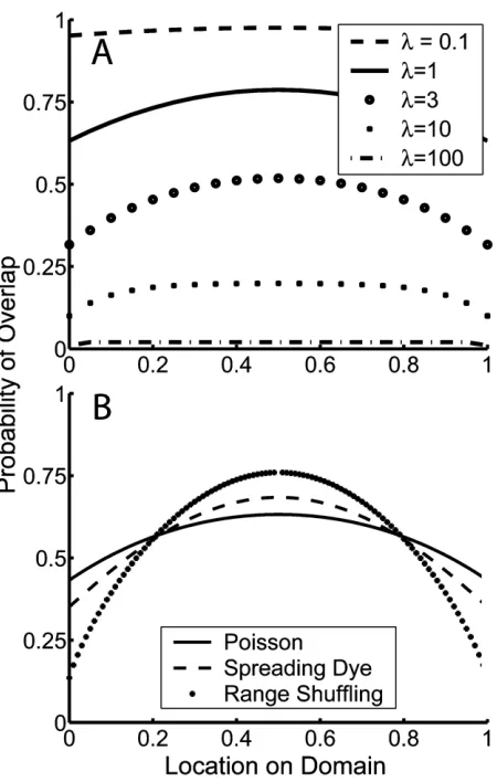
This model exhibits a quasi-parabolic mid-domain effect: the species richness gradient is steepest at domain bound-aries, and it flattens as it approaches a maximum at the mid-domain (fig. 1A). This result is robust to the Poisson process assumption: for the general class of null models in whichPr (xF_y)depends only on the distance betweenx andy(i.e., not on their specific locations), there is always a quasi-parabolic MDE (see app. B in the online edition of the American Naturalist).

Combining equations (5), (8a), and (8b) and noting that rpx ⫺x , we can obtain the probability

distri-U L

bution of range endpoints:

⫺l

e 0px ,x p1

L U

⫺lr



L U

( )

f x ,x p . (10a–10d)

L R ⫺lr

lre 0pxL,xU!1



 L U

Like the MDE itself, this distribution exhibits a feature that is common to randomization-based null models. In particular, equation (10d) is independent of range loca-tion. In other words, conditional on range extent, r, all interior range locations (i.e., range locations other than those abutting a range boundary) are equally likely. How-ever, the probability that a species’ range abuts one or both domain boundaries is always higher for the process-based null model than for either of the randomization models; consequently, its MDE is always overestimated by the ran-domization models, particularly for intermediate l (fig. 1B; see app. C in the online edition of the American Naturalist).

Alternative Null Models

Figure 1:A, Probability of range overlap versus location on the domain for the Poisson model (eq. [6]) for a variety of values of the range limitation parameter,l. Higher values oflcorrespond to higher rates of encounter of range endpoints and thus smaller ranges.B, Represen-tative comparison of the difference between the Poisson model’s mid-domain effect and those of the two null models for an equivalent prob-ability distribution of range extents as per eq. (3) (lp2).

entails two key assumptions: rarity and independence. The rarity assumption—that the probability of multiple events in one infinitesimally small interval is negligibly small— is clearly satisfied here because distributional limits will only be encountered once on either side of a species’ peak conditions. The independence assumption implies that the probability of encountering a species-specific range limit at some location within the domain depends only on en-vironmental conditions at that location (i.e., it is inde-pendent of how far a species has already successfully ex-tended its range). In nature, this latter assumption may be violated; for instance, the probability of encountering a barrier to range expansion may be low near the location of peak conditions and then increase with increasing

dis-tance from that location. The Weibull distribution captures this form of distance-dependent stochastic process (Cox and Oakes 1984). Therefore, to assess the robustness of the results from the Poisson model, I developed a second model for which the distance from species’ peak conditions to their distributional limits were drawn from a Weibull distribution.

For the Weibull model, the probability that a species’ range extends from the location of its peak conditions to encompass location xis given by

g g



exp

[

]

Pr (xF_y)p_ , (11a)

g_{( )}g

exp

[

]

and the probability density for the encounter of distri-butional limits is

g g⫺1 g g



l g(x⫺y) exp

[

]

g(xF_y)p_ , (11b)

g _{( )}g⫺1 g_{( )}g

l gy⫺x exp

_[

_]

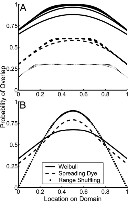
where g is the so-called shape parameter of the Weibull distribution. Whengp1, this model is equivalent to the Poisson model. When g11, then the stochastic rate at which range limits are encountered increases with increas-ing distance from the location of peak conditions (with largergcorresponding to a more steeply increasing rate). As with the Poisson model (and consistent with the general proof in app. B), this model exhibits a quasi-parabolic MDE. As g increases, the shape of the species richness gradient shifts so that species richness increases more sharply from domain boundaries toward an increasingly flat plateau through the mid-domain (fig. 2A). Despite this variability in exact shape, the MDE of the Weibull model, like that of the Poisson model, is always shallower than that of either randomization model (fig. 2B). Also con-sistent with the Poisson model, numerical integration of the Weibull model’s analogue of equation (10d) indicates that, conditional on range size, all possible interior range locations (i.e., range locations other than those abutting domain boundaries) are equally likely.

Figure 2:A, Probability of range overlap versus location on the domain for the Weibull model for a variety of values of the parameterslandg. For each line type, values of grange from 2 (lowermost line) to 10 (uppermost line), withlvaried so that the mean of the Weibull distri-bution is constant (at 0.7, 0.3, and 0.15 for thesolid,dashed, anddotted lines, respectively).B, Representative comparisons of the difference be-tween the Weibull model’s mid-domain effect and that of the two null models for an equivalent probability distribution of range sizes as per eq. (3) (lp0.36;gp5). Numerical investigations indicate that this result—shallower species richness gradients in the Weibull model than the randomization models—is consistent across parameter values.

there). To determine how this influences species richness gradients, I relaxed the range contiguity assumption by allowing species to consist of multiple discrete populations in between their potential range limits (which are still encountered at ratel, as in the Poisson null model). Spe-cifically, transitions from occupied to unoccupied habitat, and vice versa, occur at Poisson ratesaandb, respectively (and consequently, the sizes of occupied patches and dis-tances between them are exponentially distributed with means 1/aand 1/b, respectively). The derivation of species

richness gradients and probability distributions of range endpoints for this model is somewhat complicated (for details, see app. D in the online edition of the American Naturalist).

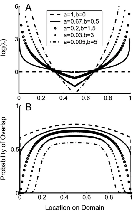
Based on patterns in range overlap, this model produces a broad range of MDEs, depending on how patchy species distributions are (fig. 3A–3C). MDEs are most pronounced when three conditions are met: range limitation is weak (lon the order of 101_{or smaller; fig. 3A), there are few—}

but more than one—patches of occupied habitat (b on the order of 100

–101

; fig. 3B), and patches of occupied habitat are small (ais large, on the order of 102

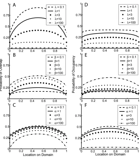
or greater; fig. 3C). However, because species in this model do not necessarily occupy all habitat between their potential range limits, range overlap (the probability that a species’ range encompasses a location) and local presence-absence (the probability that a species occupies a location) are not equivalent. If, instead of range overlap, we consider local occupancy, a different picture emerges (fig. 3D–3F). Even for parameter values that produce very peaked MDEs from the standpoint of range overlap (i.e., regional species rich-ness), MDEs in local occupancy (i.e., local species richness) are consistently shallow, similar in shape to—or in some cases, flatter than—the MDEs of the Poisson and Weibull models.

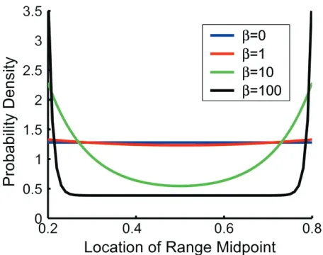
In contrast to the previous models, the patchy distri-bution model does not predict that, conditional on range size, all possible interior range locations are equally likely. Rather, because species may not occupy habitat adjacent to their potential distributional limits, range endpoints that would have abutted a domain boundary in the Poisson model are “smeared” into the domain so that range cations near domain boundaries are more likely than lo-cations near the mid-domain (fig. 4; app. D). The extent to which this occurs depends on how frequently patches of occupied habitat recur within a species’ distributional limits (i.e., onb) regardless of the other model parameters. In general, the effect is either quite small or confined to a narrow region near domain boundaries. The exception occurs when species ranges are highly noncontiguous (b

is on the order of 101

; occupied habitat patches are, on average, separated by distances≈1/10of the domain).

Discussion

Figure 3:Probability of range overlap (A–C) and occupancy (D–F) versus location on the domain for the patchy distribution model, illustrating the effects of the three model parameters.A,D, Effect of varying range limitation,l(ap10;bp5).B,E, Effect of varying the distances between patches of occupied habitat,b(lp3;ap10).C,F, Effect of varying patchiness of occupied habitat,a(lp3;bp5).

widely within the domain, in which case there is a pro-nounced MDE in range overlap but not local habitat oc-cupancy (fig. 3). However, it is unlikely that this accounts for pronounced species richness gradients in nature: the

Figure 4:Probability density for alternative interior range locations, conditional on range size (eq. [D5c]), illustrated here for a range size of 0.4 (i.e., a range encompassing 40% of the domain) and a range of values of the habitat recurrence parameter,b. Note that becauserp0.4, only range midpoints betweenxp_0.2and_xp_0.8are geometrically feasible. A horizontal line indicates a uniform distribution: all interior range lo-cations (i.e., ranges not abutting a domain boundary) are equally likely. Bowl-shaped lines indicate that ranges are more likely to be near one or the other domain boundary than centered within the domain. Numerical investigation indicates that the effect of changes inbon the probability density is consistent for different combinations oflanda. Therefore, only one case (lp1andap10) is shown here for illustration.

consistently show strong increases in local richness with regional richness (e.g., Ricklefs 1987; Cornell and Karlson 1997; Karlson et al. 2004; Witman et al. 2004).

It is likely that a strong constraint on the height of MDEs, such as that identified here, will prove to be a common feature of process-based null models, indicating that the extent to which boundary constraints can induce MDEs in nature will be limited. In particular, a constraint on the height of MDEs is robust to relaxation of the Pois-son process and (for local species richness) the contiguous range assumptions (figs. 2, 3D–3F). Moreover, there is an intuitive explanation for this result. For species richness to have a high peak in the mid-domain, species must have broad environmental tolerances (i.e., encounter unsuitable conditions rarely), so that many species extend their dis-tributions to encompass the mid-domain. However, in the absence of gradients in the quality of environmental con-ditions, these same broad tolerances increase the proba-bility that species will extend all the way to domain bound-aries, leading to relatively high species richness adjacent to those boundaries. This finding raises questions about the interpretation of statistical concordance between ran-domization models and observed patterns in species rich-ness. This concordance arises because fully randomized

and range shuffling models, like many empirical richness gradients, generally exhibit a gradual decline from high values of species richness to zero or near zero at domain boundaries (e.g., Willig and Lyons 1998; Lees et al. 1999; Koleff and Gaston 2001; Ellison 2002; Connolly et al. 2003). However, if the magnitude of MDEs is constrained, then comparing observed versus randomized species rich-ness gradients will overestimate the variation in species richness that can be explained by MDE.

Although the theory presented here raises questions about the interpretation of statistical concordance between observed species richness gradients and the predictions of randomization models, it also identifies an alternative way to use randomizations to conduct more robust tests of MDE. Except for species distributions that are highly non-contiguous, process-based null models and randomization models consistently agree on one prediction: conditional on range size, the geographical distribution of interior range locations is either uniform or nearly so. In other words, if a species richness gradient is principally due to MDE, then species ranges should be approximately ran-domly (i.e., uniformly) distributed among interior range locations, with a possible accumulation of species at or very near domain boundaries. This prediction is eminently testable, using data available from most data sets on species distributions (for an example, see Connolly et al. 2003).

Although testing for and quantifying deviations from a null model can be informative in and of itself, there is a need to understand whether and how MDEs may interact with the effects of environmental gradients to produce species richness gradients (Colwell et al. 2004). One way forward is to construct models that explicitly incorporate different assumptions about how environmental gradients and domain boundaries influence species distributions and then to compare these models with equivalent null models that omit these gradients. The general model presented here (eqq. [4]–[6]) is readily adapted for that purpose. For instance, consider an extension of the Poisson model (eqq. [8a], [8b]) that allows for symmetric variation in

l(x) across the domain:

a

0!_x!_0.5

b



l xp . (12)

a

0.5!_x!₁



1⫺x 

Figure 5:Effect of geographical gradients in the range limitation param-eter,l(x), on species richness gradients (eq. [12]).A, Gradients in range limitation,l(x).B, Probability of range overlap versus location on the domain predicted by the gradients inl(x). The legend inAapplies to both figures. Note that the dashed line is equivalent to the null model withlp₁).

Figure 6:Probability distribution of range locations associated with pa-rameters that generate bell-shaped distributions, showing the shift from a bimodal distribution at small range sizes to a unimodal distribution at large range sizes (ap0.03;bp3; cf. fig. 5). Numerical investigations indicate that the same pattern is generated for other combinations of parameter values that also produce bell-shaped species richness gradients.

approached. As b increases, l(x) varies more gradually across the domain.

In specific empirical contexts, it may be particularly informative to modell(x) as an explicit function of dif-ferent environmental variables such as habitat type, pro-ductivity, or temperature. However, even the simple model presented above produces some differences with the cor-responding null model that are illuminating (fig. 5B). In particular, as the environmental gradient steepens, species richness exhibits an increasingly bell-like shape: there is a broad, shallow gradient in species richness in the mid-domain, then a steep decline followed by a tailing off of species richness as domain boundaries are approached. This tailing-off pattern is not produced by either

potential to shed considerable light on how environmental gradients shape species distributions in nature.

One of the powerful features of mid-domain models is that they can be assessed against much more stringent conditions than, for example, regression models: they pre-dict not only the shape of a species richness gradient but also the bivariate distribution of range sizes and locations that gives rise to those gradients (cf. “strong” vs. “weak” tests of McGill [2003]). The theoretical framework pre-sented here preserves that important feature of null models (eq. [5]), but it also allows us to make the same kinds of predictions for models incorporating environmental gra-dients (e.g., fig. 6). Consequently, null models and envi-ronmental gradient models can be formulated for specific ecological contexts and explicitly fitted to empirical data. In this article, results have been expressed in terms of probability distributions on a species-by-species basis (e.g., probability of range overlap) because species differ in their breadths of environmental tolerances (and, for “non-null” models, their sensitivity to environmental gradients). Quantitative fits of models to data will require accounting for this heterogeneity in a parsimonious way, but methods exist for precisely these kinds of extensions (e.g., mixture models; Norris and Pollock 1996). A second consideration is nonindependence of environmental tolerances among species (e.g., closely related species may tolerate similar conditions), but again, the effects of nonindependence can be readily accounted for in parameter estimation (Buck-land et al. 1993; Anderson et al. 1994).

The mid-domain hypothesis has prompted ecological biogeographers to recognize that species richness at a par-ticular place depends not only on environmental quality at that location but on the broadscale distribution of en-vironmental conditions that determines the locations and sizes of species ranges. Unfortunately, ecology has lacked a formal theory of species distributions in geographical space that allows us to model species ranges as a function of the distribution of environmental conditions that pro-mote or inhibit the origination or persistence of species. This contrasts with many other areas of ecology, which are increasingly adopting approaches that confront pro-cess-oriented models directly with empirical data (e.g., be-havioral and population ecology: Hilborn and Mangel 1997; some aspects of macroecology: e.g., Hubbell 2001; Engen et al. 2002; Gaston and He 2002). The present con-tribution offers a way forward, allowing formulation of null models as well as alternatives that incorporate envi-ronmental gradients. Using such process-based approaches to analyze species richness patterns, as a complement to prevailing regression and randomization approaches, is feasible and worth further exploration.

Acknowledgments

I thank D. R. Bellwood, S. Belward, M. Bode, N. Gotelli, A. Helfgott, T. P. Hughes, M. James, N. Jenzen, K. Pollock, M. Ritchie, S. A. Sandin, C. Schwarz, and anonymous reviewers for thoughtful and constructive comments at various stages during the preparation of this article. I grate-fully acknowledge M. Bode, K. Hartmann, M. Hisano, and M. Hoogenboom for assistance with programming and preparation of figures. The Australian Research Council and James Cook University provided financial support for this work. This is contribution 145 of the Centre for Coral Reef Biodiversity.

Literature Cited

Anderson, D. R., K. P. Burnham, and G. C. White. 1994. AIC model selection in overdispersed capture-recapture data. Ecology 75: 1780–1793.

Arita, H. T. 2004. Range size in mid-domain models of species di-versity. Journal of Theoretical Biology 232:119–126.

Bokma, F., J. Bokma, and M. Mo¨nkko¨nen. 2001. Random processes and geographic species richness patterns: why so few species in the north? Ecography 24:43–49.

Buckland, S. T., D. R. Anderson, K. P. Burnham, and J. L. Laake. 1993. Distance sampling: estimating abundance of biological pop-ulations. Chapman & Hall, London.

Chown, S. L., and K. J. Gaston. 2000. Areas, cradles, and museums: the latitudinal gradient in species richness. Trends in Ecology & Evolution 15:311–315.

Colwell, R. K., and G. C. Hurtt. 1994. Nonbiological gradients in species richness and a spurious Rapoport effect. American Nat-uralist 144:570–595.

Colwell, R. K., and D. C. Lees. 2000. The mid-domain effect: geo-metric constraints on the geography of species richness. Trends in Ecology & Evolution 15:70–76.

Colwell, R. K., N. Gotelli, and C. Rahbek. 2004. The mid-domain effect and species richness patterns: what have we learned so far? American Naturalist 163:E1–E23.

Connolly, S. R., D. R. Bellwood, and T. P. Hughes. 2003. Indo-Pacific biodiversity of coral reefs: deviations from a mid-domain model. Ecology 84:2178–2190.

Cornell, H. V., and R. H. Karlson. 1997. Local and regional processes as controls of species richness. Pages 250–268inD. Tilman and P. Kareiva, eds. Spatial ecology: the role of space in population dynamics and interspecific interactions. Princeton University Press, Princeton, NJ.

Cox, D. R., and D. Oakes. 1984. Analysis of survival data. Chapman & Hall, London.

Ellison, A. M. 2002. Macroecology of mangroves: large-scale patterns and processes in tropical coastal forests. Trees: Structure and Func-tion 16:181–194.

Engen, S., R. Lande, T. Walla, and P. J. deVries. 2002. Analyzing spatial structure of communities using the two-dimensional Pois-son lognormal species abundance model. American Naturalist 160: 60–73.

Grytnes, J. A. 2003. Ecological interpretations of the mid-domain effect. Ecology Letters 6:883–888.

Grytnes, J. A., and O. R. Vetaas. 2002. Species richness and altitude: a comparison between null models and interpolated plant species richness along the Himalayan altitudinal gradient, Nepal. Amer-ican Naturalist 159:294–304.

Hawkins, B. A., and J. A. F. Diniz-Filho. 2002. The mid-domain effect cannot explain the diversity gradient of Nearctic birds. Global Ecology and Biogeography 11:419–426.

Hilborn, R., and M. Mangel. 1997. The ecological detective: con-fronting models with data. Princeton University Press, Princeton, NJ.

Hubbell, S. P. 2001. The unified neutral theory of biodiversity and biogeography. Princeton University Press, Princeton, NJ. Hughes, T. P., D. R. Bellwood, and S. R. Connolly. 2002. Biodiversity

hotspots, centers of endemicity, and the conservation of coral reefs. Ecology Letters 5:775–784.

Jetz, W., and C. Rahbek. 2001. Geometric constraints explain much of the species richness pattern in African birds. Proceedings of the National Academy of Sciences of the USA 98:5661–5666. ———. 2002. Geographic range size and determinants of avian

spe-cies richness. Science 297:1548–1551.

Karlson, R. H., H. V. Cornell, and T. P. Hughes. 2004. Coral com-munities are regionally enriched along an oceanic biodiversity gra-dient. Nature 429:867–870.

Kessler, M. 2001. Patterns of diversity and range size of selected plant groups along an elevational transect in the Bolivian Andes. Bio-diversity and Conservation 10:1897–1921.

Koleff, P., and K. J. Gaston. 2001. Latitudinal gradients in diversity: real patterns and random models. Ecography 24:341–351. Lees, D. C., C. Kremen, and L. Andriamampianina. 1999. A null

model for species richness gradients: bounded range overlap of butterflies and other rainforest endemics in Madagascar. Biological Journal of the Linnean Society 67:529–584.

Lyons, S. K., and M. L. Willig. 1997. Latitudinal patterns of range size: methodological concerns and empirical evaluations for New World bats and marsupials. Oikos 79:568–580.

McGill, B. J. 2003. Strong and weak tests of macroecological theory. Oikos 102:679–685.

Norris, J. L., and K. H. Pollock. 1996. Nonparametric MLE under two closed capture-recapture models with heterogeneity. Biomet-rics 52:639–649.

Pin˜eda, J., and H. Caswell. 1998. Bathymetric species-diversity pat-terns and boundary constraints on vertical range distributions. Deep Sea Research II: Topical Studies in Oceanography 45:83–101. Ricklefs, R. E. 1987. Community diversity: relative roles of local and

regional processes. Science 235:167–171.

Roughgarden, J. 1983. Competition and theory in community ecol-ogy. American Naturalist 122:583–601.

Sanders, N. J. 2002. Elevational gradients in ant species richness: area, geometry, and Rapoport’s Rule. Ecography 25:25–32. Taylor, H. M. and S. Karlin. 1994. An introduction to stochastic

modeling. Academic Press, San Diego, CA.

Willig, M. R., and S. K. Lyons. 1998. An analytical model of latitudinal gradients of species richness with an empirical test for marsupials and bats in the New World. Oikos 81:93–98.

Willig, M. R., D. M. Kaufman, and R. D. Stevens. 2003. Latitudinal gradients of biodiversity: pattern, process, scale, and synthesis. Annual Review of Ecology and Systematics 34:273–309. Witman, J., R. J. Etter, and F. Smith. 2004. The relationship between

regional and local species diversity in marine benthic communities: a global perspective. Proceedings of the National Academy of Sci-ences of the USA 101:15664–15669.

Zapata, F. A., K. J. Gaston, and S. L. Chown. 2003. Mid-domain models of species richness gradients: assumptions, methods, and evidence. Journal of Animal Ecology 72:677–690.