Machine Learning Based Autism Detection Using Brain Imaging

(1)

Rochester Institute of Technology

RIT Scholar Works

Theses Thesis/Dissertation Collections

3-27-2017

Machine Learning Based Autism Detection Using

Brain Imaging

Gajendra Jung Katuwal [email protected]

Follow this and additional works at:http://scholarworks.rit.edu/theses

This Dissertation is brought to you for free and open access by the Thesis/Dissertation Collections at RIT Scholar Works. It has been accepted for inclusion in Theses by an authorized administrator of RIT Scholar Works. For more information, please [email protected]. Recommended Citation

(2)

Machine Learning

Based Autism Detection

Using Brain Imaging

A dissertation

by

Gajendra Jung Katuwal

Submitted in partial fulfilment

of

Doctor of Philosophy in Imaging Science

Chester F. Carlson Center for Imaging Science

Rochester Institute of Technology

Rochester, New York, USA

(3)

Chester F. Carlson Center for Imaging Science

Rochester Institute of Technology

Rochester, New York, USA

CERTIFICATE OF APPROVAL

PhD Degree Dissertation

The PhD Degree Dissertation of Gajendra Jung Katuwal has been examined and approved by the following dissertation committee as satisfactory for a PhD degree in Imaging Science.

Dr. Andrew Michael, Dissertation Advisor Date

Dr. Stefi Baum, Dissertation Advisor Date

Dr. Manuela Campanelli, Committee Chair Date

Dr. Nathan Cahill, Committee Member Date

(4)

(5)

ACKNOWLEDGMENTS

First of all, I would like to express my sincere gratitude to my advisors, Dr. Andrew Michael and

Dr. Stefi Baum for their guidance and training during this fulfilling journey of four years and some

months. Andrew believed in me despite of my zero experience in brain imaging and guided me to

this point. Stefi, despite being physically on the other side of the 49th_{parallel, always inspired me}

to ask the right questions, which was pivotal for the evolution of my thought process and was

immensely helpful during the course of my research.

I would also like to thank the rest of the dissertation committee: Dr. Nathan Cahill, Dr. John

Kerekes, and Dr. Manuela Campanelli, for many insightful comments and questions. My sincere

gratitude also goes to my cool lab mates Chao, Chase, and Viraj. Without them, this journey would

have been difficult. My sincere gratitude goes to all the individuals behind the data, ideas,

publications, software, etc. used in my research and all helpful folks from stackexchange. Without

their contributions, I would not have made this far.

I would like to thank Ronnie and Rob for their help in grammatical debugging. Finally, I am

grateful to several baristas from the beautiful town of Lewisburg to the hip places in Cambridge

(6)

ABSTRACT

Autism Spectrum Disorder (ASD) is a group of heterogeneous developmental disabilities

that manifest in early childhood. Currently, ASD is primarily diagnosed by assessing the behavioral

and intellectual abilities of a child. This behavioral diagnosis can be subjective, time consuming,

inconclusive, does not provide insight on the underlying etiology, and is not suitable for early

detection. Diagnosis based on brain magnetic resonance imaging (MRI)—a widely used

non-invasive tool—can be objective, can help understand the brain alterations in ASD, and can be

suitable for early diagnosis. However, the brain morphological findings in ASD from MRI studies

have been inconsistent. Moreover, there has been limited success in machine learning based ASD

detection using MRI derived brain features. In this thesis, we begin by demonstrating that the low

success in ASD detection and the inconsistent findings are likely attributable to the heterogeneity

of brain alterations in ASD. We then show that ASD detection can be significantly improved by

mitigating the heterogeneity with the help of behavioral and demographics information. Here we

demonstrate that finding brain markers in well-defined sub-groups of ASD is easier and more

insightful than identifying markers across the whole spectrum. Finally, our study focused on brain

MRI of a pediatric cohort (3 to 4 years) and achieved a high classification success (AUC of 95%).

Results of this study indicate three main alterations in early ASD brains: 1) abnormally large

ventricles, 2) highly folded cortices, and 3) low image intensity in white matter regions suggesting

myelination deficits indicative of decreased structural connectivity. Results of this thesis

demonstrate that the meaningful brain markers of ASD can be extracted by applying machine

learning techniques on brain MRI data. This data-driven technique can be a powerful tool for

(7)

ABBREVIATIONS

ABIDE: Autism Brain Imaging Data Exchange

ADHD: Attention Deficit Hyperactivity Disorder

AS: Autism Severity

ASD: Autism Spectrum Disorder

AUC: Area Under the Receiver Operating Curve

CARS: Childhood Autism Rating Scale

CDC: Center for Disease Control and Prevention

CTR: Controls

CSF: Cerebrospinal Fluid

Curvind: Curvature Index

DB: Demographics and Behavioral Measures

DC: Diencephalon

FAST: FMRIB's Automated Segmentation Tool

Foldind: Folding Index

FS: FreeSurfer

FSL: FMRIB Software Library

Gauscurv: Gaussian Curvature

GM: Gray Matter

Meancurv: Mean Curvature

MRI: Magnetic Resonance Imaging

(8)

Std.: Standard Deviation

TDC: Typically Developing Controls

TIV: Total Intracranial Volume

VIQ: Verbal Intelligent Quotient

(9)

FIGURES

Figure 1.1 Thesis Organization ... 9

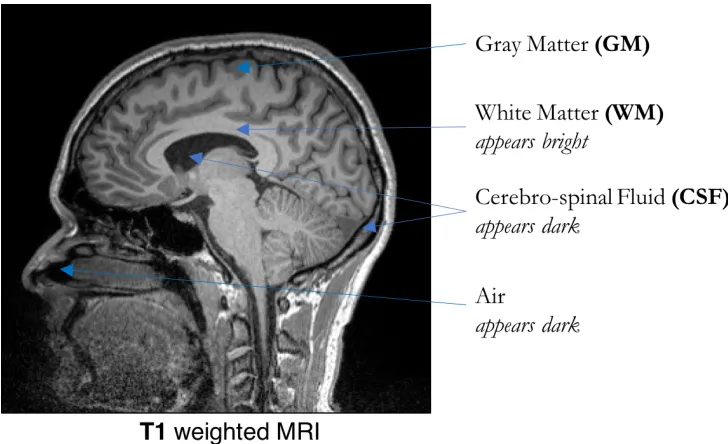
Figure 2.1: Sagittal view of a T1 weighted brain MRI. ... 13

Figure 2.2: MRI acquisition process. ... 15

Figure 2.3: SPM Tissue Segmentation. ... 18

Figure 2.4: Freesurfer (FS) recon-all processing workflow ... 20

Figure 2.5: Sub-cortical segmentation & cortical parcellation in Freesurfer (FS). ... 22

Figure 2.6: Random Forest is an ensemble of decision trees. ... 28

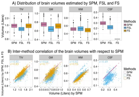
Figure 3.1: Distribution of estimated brain volumes and inter-method differences. ... 42

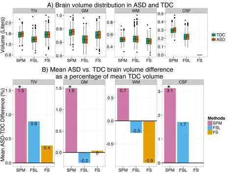
Figure 3.2: ASD – TDC brain volume differences are method dependent ... 44

Figure 3.3: Inter-method segmentation comparison ... 52

Figure 3.4: Multi-variate pattern is more robust across methods ... 59

Figure 4.1: Improvement in classification by sub-grouping ... 72

Figure 4.2: Important features for classification are different across sub-groups. ... 77

Figure 4.3: Variability of the important features. ... 78

Figure 4.4: Folding index and curvature features are important for classification in young subjects ... 85

Figure 4.5: ASD vs. TDC group difference in ventricular volumes decreases with verbal IQ (VIQ) ... 91

Figure 5.1: Subject Selection Flowchart ... 97

Figure 5.2: Classification Flowchart. ... 100

(16)

Figure 5.4: Global Volume Features ... 104

Figure 5.5: ASD vs. CTR Classification Scores. ... 105

Figure 5.6: Important brain feature for ASD vs. CTR classification ... 107

Figure 5.7: Important morphology features for ASD vs. CTR classification. ... 108

Figure 5.8: Important intensity features for ASD vs. CTR classification. ... 109

Figure 5.9: Cortical expansion theory on cortical gyrification ... 113

Figure 5.10: Higher cortical folding in ASD brain. ... 115

Figure 5.11: Inefficient communication in ASD brain. ... 116

Figure 5.12: Arrested brain growth in ASD ... 118

Figure 8.1: Gradient Boosting Machine: Improvement in classification by sub-grouping based on autism severity (AS), age and Verbal IQ (VIQ). ... 154

Figure 8.2. Gradient Boosting Machine (GBM): Important features for classification are variable across sub-groups. ... 155

Figure 8.3: Inter and intra sub-groups classification AUC scores ... 156

Figure 8.4: Random Forest: Important features for classification in sub-groups (10% threshold). ... 157

Figure 8.5: Random Forest: Important features for classification by in sub-groups (25% threshold). ... 158

Figure 8.6: Classification performance degrades with Autism Severity (AS). ... 159

(17)

TABLES

Table 3.1: Subject demographics and behavioral (DB) measures ... 35

Table 3.2: Estimated brain volumes and inter-method differences ... 41

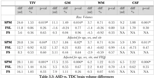
Table 3.3: ASD vs. TDC brain volume differences ... 43

Table 3.4: Differential bias for diagnostic group (ASD) ... 46

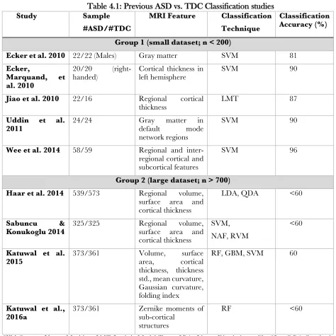
Table 4.1: Previous ASD vs. TDC Classification studies ... 64

Table 4.2: Subject demographics and behavioral (DB) measures ... 66

Table 4.3: Sub-groups definition ... 70

Table 4.4: Classification AUC in sub-groups created by AS, VIQ and age ... 73

Table 7.1: Estimated brain volumes and inter-method differences in NYU ... 151

Table 7.2: ASD vs. TDC brain volume differences in NYU ... 152

Table 7.3: Differential bias for diagnostic group (ASD) in NYU ... 153

(18)

1

CHAPTER 1: INTRODUCTION

1.1

Autism Spectrum Disorder

Autism Spectrum Disorder (ASD) is a group of lifelong developmental disabilities that

manifest in early childhood. According to DSM 5 (American Psychiatric Association, 2013), ASD

is characterized by impairment in social-communication and behavior domains, including

repetitive behaviors and restrictive interests. According to a recent Center for Disease Control and

Prevention (CDC) survey (CDC, 2014), 1 in 68 children (1 in 42 boys and 1 in 189 girls) have ASD.

A more recent CDC survey of parents indicated that this number can be as high as 1 in 45

(Zablotsky et al., 2015). In addition to the substantial difficulties faced by ASD individuals and their

parents, the economic burden of ASD is high. A recent study by Leigh and Du (2015) has estimated

ASD’s economic cost for 2015 to be $268 billion in the United States alone. The study projects

annual costs rising to $461 billion in 2025 if ASD’s prevalence remains constant and more than $1

trillion by 2025 if ASD’s prevalence continues the steep rise seen over the last decade.

ASD is highly heterogeneous in its etiology, comorbidity, pathogenesis, genetics, and

severity (Betancur, 2011; Happé et al., 2006; Jeste & Geschwind, 2014; Ronald et al., 2006). It has

a strong genetic basis and is highly heritable (Ronald et al., 2006). It has been reported that 10%–

20% of individuals with ASD have an identified genetic etiology. The genetic architecture of ASD

is highly heterogeneous (Geschwind & Levitt, 2007; Jeste & Geschwind, 2014); ASD has been

linked to more than 100 different genes affecting different aspects of neurodevelopment and

(19)

disorders (Dougherty et al., 2016b; Matson et al., 2013). For example, it has been estimated that

14 to 78% of children with ASD also meet the criteria for Attention Deficit and Hyperactivity

Disorder (ADHD) (Gargaro et al., 2011), up to 42% meet the criteria for anxiety disorders (Matson

et al., 2013), and 25 to 70% have some level of intellectual disability (Fombonne, 2009). Similarly,

brain alterations in ASD have been found to be highly heterogeneous which is discussed in Section

1.6.2

1.2

Importance of early detection of ASD

Early detection of ASD is important because it allows for the application of early

intervention methods. It has been shown that early intervention is effective in decreasing

impairments (Dawson et al., 2010) and may result in more positive long-term outcomes for the

child (Pickles et al., 2016; Rogers & Vismara, 2010). The annual economic cost of ASD has been

significant—and the largest factors contributing to the cost are lost productivity and adult care

(Ganz, 2007). With successful application of early intervention methods, in addition to improving

the quality of life of ASD individuals, the economic cost related to ASD can also be significantly

reduced. And, for successful application of early intervention methods, early detection of ASD is

required.

Early detection of ASD may help to disentangle the effects of genetic and environmental

risk factors of ASD and may improve our knowledge of its underlying etiology. A large study by

Sandin et al. (2014) including 2 million children (~14500 ASD) have reported that the risk of ASD

is influenced equally by genetic and environmental factors. Environmental factors include a wide

range of influences such as parental age (Sandin et al., 2015), obstetric conditions (Kolevzon et al.,

2007), medication used (Boukhris et al., 2015), maternal nutrition (Lyall et al., 2013; Schmidt et

(20)

The environmental factors related to the risk of ASD can interact with each other making the

etiology of ASD more complex. If detection can be achieved at the neonatal stage, it can help in

separating out the effects of post-natal environmental risk factors of ASD—thus, improving our

knowledge of ASD etiology.

In addition, it may be the case that ASD is closer to normal development in its presentation

at a younger age, before environmental factors have influenced its postnatal development. That

is, when a child is tested for ASD as early as possible, fewer environmental factors will have

contributed to the development of ASD after birth—which means that the underlying etiology and

perhaps its manifestation may be more homogenous—which in turn, would make it easier to detect

and understand the underlying etiology of ASD in children through the application of biomarkers

at very young age.

Below we briefly discuss the major challenges faced by current techniques for ASD

detection and studies investigating brain morphology of ASD.

1.3

Problem 1: Behavior based diagnosis of ASD is late and does not help

to understand underpinnings of ASD

Currently ASD diagnosis is based on clinical assessments based on observations of the

individual's behavior and intellectual abilities. This diagnosis procedure can be subjective, time

consuming, and inconclusive due to factors such as comorbidity (Close et al., 2012). An objective

diagnostic tool is highly valuable and its importance further increases from the fact that currently

existing behavioral diagnosis has been found to be highly subjective especially at a young age where

there is so little to observe. In addition, since the present diagnosis procedure is based only on

behavioral symptoms, it does not provide insight on the brain anatomical underpinnings and

(21)

intervention. According to a recent report by CDC (CDC, 2014), the median age of ASD diagnosis

is 53 months. Similarly, it has been reported that more than half of school-aged kids were age 5 or

older when they were first diagnosed with ASD and less than 20% were diagnosed by age 2 years

(Pringle et al., 2012).

1.4

Problem 2: Inconsistent brain anatomical findings in ASD

A number of studies utilizing structural Magnetic Resonance Imaging (MRI) data to

investigate the brain morphology of ASD have reported alterations in brain regions involved in

language and social behavior, particularly fronto-temporal regions (Bigler et al., 2007; Ha et al.,

2015), and the amygdala-hippocampus complex (Groen et al., 2010; Nordahl et al., 2012). Early

brain overgrowth (Campbell et al., 2014), alterations in corpus callosum (Wolff et al., 2015),

cerebellum (D’Mello et al., 2015), and fusiform (Dougherty et al., 2016a; van Kooten et al., 2008)

have also been reported by studies. However, these findings have been somewhat inconsistent

(Amaral et al., 2008; Chen et al., 2011; Katuwal et al., 2015a).

1.5

Problem 3: Low Classification success in large multi-site data

In recent years, several studies have applied machine learning on MRI derived brain

features, targeted at ASD detection. These studies have been successful with high classification

accuracies (80%) for well-matched small datasets (n < 200). However, the studies using the large

multi-site ABIDE dataset (n > 700) (Haar et al., 2014; Katuwal et al., 2015b; Sabuncu &

Konukoglu, 2014) have reported low classification accuracies (~60%).

(22)

1.6.1

Demonstrating MRI as a potential tool for detection

As a solution to the Problem 1 i.e. “Behavior based diagnosis of ASD is late and does not help to

understand the underpinnings of ASD”, we demonstrate that ASD can be successfully detected using

machine learning on MRI data. Using brain images of both children and adult subjects,

data-driven potential brain biomarkers that are consistent with the current biological understanding of

ASD were found. In addition, we could successfully classify ASD subjects from non-ASD subjects

in many cases. From the results of this thesis, we can safely argue that the application of machine

learning on MRI data can be a useful technique for early detection of ASD and for understanding

its brain anatomical underpinnings. This analysis and results are presented in Chapter 4 and

Chapter 5.

1.6.2

Relating inconsistent findings and low classification success to ASD

heterogeneity and methodological differences

In this thesis, we have attempted to identify the causes of Problem 2: “Inconsistent brain

anatomical findings in ASD” and Problem 3: “Low Classification success in large multi-site data”. We

attribute methodological differences and heterogeneity of ASD, or a combination of both, as the

likely underlying causes of these discrepancies.

The methodological differences can arise from the differences in image preprocessing tools,

analytical models, covariates, etc. In this thesis, we focus on methodological differences due to the

choice of image preprocessing tool. This analysis and results are presented in Chapter 3.

The heterogeneity of ASD brain morphology can be mainly attributed to the significant

dependence of brain alterations on demographics and behavioral (DB) measures such as age, sex,

IQ, handedness, etc. Previous studies have reported variability in brain alterations with factors

(23)

thesis, we focus on the variability ASD brain alterations with respect to three DB measures: age,

verbal IQ (VIQ), and autism severity (AS). This analysis and results are presented in Chapter 4.

1.6.3

Providing the evidence of brain image processing tool dependent findings and

suggesting multi-variate techniques as a partial solution

We investigate differences in image preprocessing tools as a possible cause behind the

inconsistent anatomical findings in ASD and in neuroimaging in general. In particular, we focus

on the estimation of the following brain volumes: gray matter (GM), white matter (WM),

cerebrospinal fluid (CSF), and total intracranial volume (TIV) from T1-weighted MRIs using three

popular preprocessing methods: SPM, FSL, and FreeSurfer (FS). We found that the estimated

brain volumes did not agree across methods and the methods showed differential biases for ASD,

and many of the biases were larger than ASD versus TDC differences. In summary, we

demonstrated that the differences in the choice of image preprocessing tool is a reason behind the

inconsistent neuroimaging findings in ASD.

Improving the current brain image preprocessing tools to make them more accurate and

standardizing them is the best possible solution to remove the effects of methodological differences

in the end findings. However, when the existing popular tools have to be used, we suggest

investigating multi-variate relationships (in addition to univariate relationships) in brain alterations

because multi-variate relationships are more robust across methods and scanners. In this thesis, we

provide few examples to corroborate this view. This analysis and results are presented in Chapter

(24)

1.6.4

Divide and Conquer: we propose identifying brain biomarkers in sub-groups of

ASD is easier and more meaningful than across the whole spectrum

We first propose and then demonstrate that the heterogeneity in ASD brain morphometry

can be mitigated by augmenting the information from demographics and behavioral measures

(DB) of the subjects. We demonstrate that identifying ASD brain alterations in relatively

homogenous sub-groups is easier and more insightful than across the whole heterogeneous ASD

spectrum. We use automatically extracted multiple brain morphological features and multiple

classification techniques for this investigation. We explore if DB measures of the subjects can be

utilized to mitigate the ASD heterogeneity and hence facilitating a better understanding of the

brain alterations associated with ASD and aiding in its detection. First, we investigate the

incremental predictive power that can be gained by adding DB measures such as age, VIQ, and

AS to the brain morphological features derived from MRI. Second, we probe if sub-grouping the

subjects by the above-mentioned DB measures helps to improve ASD vs. TDC classification and

provides better insight into the brain morphometric alterations in ASD. This analysis and results

are presented in Chapter 4.

1.6.5

Brain biomarkers discovery for early detection of ASD

We apply machine learning on automatically extracted multiple brain morphometric and

intensity features to classify young ASD subjects (3 to 4 years) from the controls of the same age

group. We achieved very high success rate (> 90% AUC) for ASD vs. control classification. We

also identified three potential brain markers for early detection of ASD: larger ventricles, larger

TIV, higher amount of cortical folding, and myelination deficits particularly in frontal and

temporal regions. We also noticed that larger TIV of ASD brain is related to larger cortical surface

(25)

amount of cortical folding in ASD brains may be an aftereffect of the early brain overgrowth in

ASD. We also hypothesize that the higher amount of cortical folding in ASD is due to the greater

compressive stress in the cortex induced by both hyper-expansion of the cortex and abnormally

large ventricles. To our knowledge this is the first study to leverage clinical imaging archives to

investigate early brain markers in ASD. The high degree of success in classification and the

biologically relevant potential brain markers indicate that application of advanced analytic

methods on brain features holds promise for aiding early identification of ASD.

1.7

Thesis Organization

This thesis is divided into six chapters and three appendices; see Figure 1.1.

1.7.1

Chapter 1: Introduction

This Chapter contains a brief introduction to ASD and studies investigating brain

alterations in ASD using MRI. It starts with the shortcomings of behavioral based ASD diagnosis

and then provides motivation for brain morphology based ASD detection using machine learning.

This chapter makes an effort to educate the reader about the importance of early detection of ASD

and then presents MRI based ASD detection as a potential technique for it. Finally, this chapter

briefly discusses the challenges to characterize the ASD brain morphology using MRI and then

(26)

[image:26.612.67.551.73.348.2]

Figure 1.1 Thesis Organization

1.7.2

Chapter 2: Background

This Chapter contains the basic elements required to get acquainted with brain imaging in

general and brain MRI data processing and analysis in particular. It includes a brief introduction

to MRI, extraction of brain features from MRI, and univariate and multi-variate analysis

techniques used to identify meaningful patterns from these brain features.

1.7.3

Chapter 3: Method Dependent Findings

This Chapter is based on the Frontiers in Neuroscience research article “Inter-Method

Discrepancies in Brain Volume Estimation May Drive Inconsistent Findings in Autism” (Katuwal

et al., 2016b). Using the case study of brain volumes estimation from three popular brain image

processing tools, this Chapter provides the evidence that the differences in the choice of processing

(27)

1.7.4

Chapter 4: Brain Morphology Based ASD Detection and Tackling ASD

Heterogeneity

This Chapter is based on the PLOS ONE journal research article “Divide and Conquer:

Sub-Grouping of ASD Improves ASD Detection Based on Brain Morphometry” (Katuwal et al.,

2016c). Using the brain images of adult subjects (6 to 40 years) from the ABIDE dataset, this

Chapter shows how information from DB measures such as age, VIQ, and AS can help to mitigate

the heterogeneity in ASD brain morphology. This Chapter demonstrates that searching for the

brain biomarkers in meaningful sub-groups of ASD is easier and more meaningful than searching

them across the whole ASD spectrum.

1.7.5

Chapter 5: Early Detection of ASD

Utilizing the brain images of subjects 3 to 4 years of age from a clinical imaging archive at

Geisinger Health System, this Chapter demonstrates that applying machine learning on

MRI-derived brain morphology features, early brain markers of ASD can be identified in a data-driven

fashion and be used for early detection of ASD.

1.7.6

Chapter 6: Conclusion

This Chapter summarizes the methodology and the results of this thesis and provides a

discussion on the implications of the findings of this thesis. Finally, it concludes by discussing the

future work.

1.7.7

Appendices

Appendix A, B, and C contain the supplementary materials form Chapter 3, 4, and 5

(28)

(29)

2

CHAPTER 2: BACKGROUND

2.1

Brain Imaging

Brain imaging includes the use of diverse techniques to image the structure, function, and

biochemical processes of the brain. Imaging technologies of various modalities now provide the

visualization of the structure and function of the brain with high resolution. Brain imaging is

becoming an important technique in both research and clinical care. It is being successfully used

to facilitate the understanding of the structure and the functions of the brain and also has been a

vital diagnostic tool for many neurological disorders (O’Brien, 2007). Brain imaging can be broadly

categorized into three categories: structural, functional, and molecular imaging (Asbury, 2011).

Structural imaging techniques can capture the anatomical structure of the brain and

include X-ray, Computer Assisted Tomography (CT), MRI, Diffusion Tensor Imaging (DTI) etc.

MRI is based on the principle of nuclear magnetic resonance and uses radiofrequency waves to

probe tissue structure. DTI is a special form of MRI technique that measures the diffusion of water

as a function of spatial location and is used to characterize the microstructural changes in the tissues

(Le Bihan et al., 2001). It is widely used to estimate the WM connectivity patterns in neurological

disorders such as ASD and ADHD (Assaf & Pasternak, 2008).

Functional imaging techniques capture the function or physiology of the brain or measure

the brain metabolism (Raichle, 1998). Most of the techniques such as functional Magnetic

Resonance Imaging (fMRI) and Positron Emission Tomography (PET), measure the amount of

cerebral blood flow as a proxy to the brain metabolism rate assuming that there is more blood flow

(30)

Molecular and cellular imaging techniques probe the biochemical activities of cells and

their molecules (Massoud & Gambhir, 2003). They generally use different kinds of light

microscopes on light-emitting probes. The light-emitting probes are the molecules emitting radio

frequencies of various wavelengths to contrast the target cells.

In addition to the unimodal studies based on brain images of a single modality, there are

several other studies utilizing the joint information from the brain images of multiple modalities

(Michael, 2009; Michael et al., 2010, 2011; Pichler et al., 2010; Townsend & Cherry, 2001).

This thesis makes an effort to identify brain markers for ASD detection using the brain

morphology captured by MRI. So, we will limit our scope to MRI from here on. To be more

particular, MRI refers to structural MRI in this thesis. All the brain MRI images used in this thesis

were T1-weighted. In T1-weighted images, tissues with high fat content (e.g. WM) appear bright

whereas fluids (e.g. CSF) and air appear dark (Hornak, 1996). Figure 2.1 shows the sagittal view

[image:30.612.130.494.427.649.2]

of a typical T1-weighted brain MRI.

(31)

2.2

MRI

MRI is a non-invasive tool for examining the anatomy of the human body. It is based on

the principle of magnetic resonance imaging and it utilizes the magnetic properties of the proton

of the hydrogen atom which is abundant in our body.

2.2.1

MRI acquisition

Here we briefly explain the MRI acquisition process. For detailed information, please refer

to https://radiopaedia.org/articles/mri-introduction, Pooley (2005), Hornak (1996) and Section

2.1 of Michael (2009). A typical MRI machine consists of three major components: a very strong

main magnet, gradient magnets, and a radio frequency emitter. A typical MRI process includes

four major components: slice selection, phase encoding, frequency encoding, and signal

reconstruction (see Figure 2.2).

Slice selection: The protons spin around their axes effectively acting as small magnetic

dipoles. Initially, the magnetic dipoles (protons) are randomly aligned. When a strong external

magnetic field of the MRI machine is applied, in addition to the spinning motion, the dipoles start

to precess along the direction of the external field at the Larmor frequency, which is proportional

to the external magnetic field. After that, a combination of gradient magnets is turned on, by effect

of which, the net magnetic field varies linearly along the axis perpendicular to the 2D slice of

interest—i.e. the net magnetic field is uniform in each slice but is different across the slices—which

means the protons at each slice are precessing with unique frequency and hence can only absorb

electromagnetic waves of particular frequencies to resonate, echo or excite. In other words, varying

(32)

Figure 2.2: MRI acquisition process.

Phase encoding. A suitable radio frequency pulse is emitted for a brief time so that the

hydrogen atoms only in the slice of interest are excited. Then the radio frequency is turned off and

the excited hydrogen atoms are allowed to return to the low energy state through a gradual decay.

During relaxation, electromagnetic waves are emitted at the precessing frequency of the Hydrogen

atoms. Then another set of gradient magnets is turned on for a short interval, by effect of which,

the net magnetic field along one axis of the slice of interest varies. Since the precession frequency

is dependent on the external magnetic field, protons at different locations precess with different

frequencies creating location dependent phase lag relative to their initial state. This location

dependent phase lag effectively encodes the spatial information in the slice of interest. In practice,

several phase encoding steps are repeated so that the captured signal has enough information to

reconstruct the anatomical image.

Frequency encoding. After phase encoding, another gradient is applied along the axis

perpendicular to the phase encoding axis so that the hydrogen atoms at different columns precess

(33)

Signal reconstruction. The excited hydrogen atoms return to the low energy state

releasing electromagnetic waves. These waves have frequency and phase dependent on their spatial

location and are picked up by receiver coils and the collected 2D signal is called the k-space. A

Fourier Transform is applied on the k-space image to reconstruct the 2D anatomical image of the

slice. Multiple 2D slices are collected and combined to form the 3D MRI volume.

2.3

Brain Feature extraction from MRI

MRI data have to be processed to extract brain features before performing further analyses

on them. There are a number of automatic software tools available from different labs and research

universities for MRI data processing. Among them, the most popular are SPM (Ashburner &

Friston, 2005), FS (Dale et al., 1999a; Fischl et al., 1999b), FSL (Jenkinson & Smith, 2001), AFNI

(Cox, 1996), and LONI (Dinov et al., 2010). MRI data processing can be roughly divided into two

steps. The first step includes preprocessing tasks such as motion correction, non-uniform intensity

normalization, skull stripping, etc. These tasks ensure that the final image is suitable for further

processing. In other words, these preprocessing tasks are image processing operations performed

on raw brain images so that they have desirable properties that are consistent with the assumptions

made by the subsequent registration and segmentation steps. The second step includes tasks such

as registration of a brain image to a standard brain template and segmentation of cortical and

sub-cortical brain regions.

Below we briefly discuss the brain feature extraction steps of three popular neuroimaging

preprocessing tools that were used in this thesis.

2.3.1

SPM

SPM (http://www.fil.ion.ucl.ac.uk/spm/) is a brain imaging software tool mainly designed

(34)

& collaborators of the Wellcome Trust Centre for Neuroimaging at University College London.

In Chapter 3 of this thesis, SPM was utilized for the segmentation of following brain tissues: GM,

WM, and CSF.

Tissue segmentation in SPM is performed using the New Segment tool (Ashburner et al.,

2013). New Segment utilizes a Gaussian Mixture Model (GMM) with components for GM, WM,

CSF, bone, soft tissue, and air/background where each component is modeled as one or more

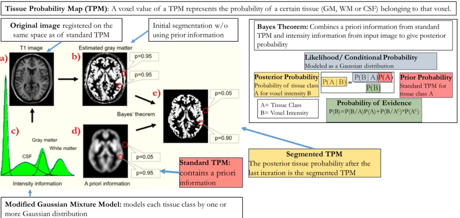
Gaussians. The distribution or histogram of image intensities in a T1 weighted brain image (Figure

2.1A) are modeled by a GMM (Figure 2.3c) where the different peaks correspond to the different

image intensities of the tissue classes. The mixture model is updated by combining the spatial

information from a standard tissue probability map (TPM) and the intensity information of the

input MRI (Ashburner & Friston, 2005). The standard TPM (Figure 2.3d) of a tissue contains

information about the spatial location of the tissue in a probabilistic sense. The value at a certain

voxel of a TPM represents the probability of a certain tissue (GM, WM or CSF) belonging to that

voxel. In this example, a voxel value of the TPM in Figure 2.3d represents the probability that the

voxel contains GM. New Segment uses ICBM-452 T1 brain atlases (Mazziotta et al., 2001a) as

standard TPMs.

At first the T1 image is registered in the same space as the standard TPM. After the

registration, the registered T1 image is segmented roughly based on intensity thresholds to get an

initial segmentation map (Figure 2.3b) to create an initial TPM. Then, the segmented tissue map

is refined using Bayes’ theorem with the standard TPM as a priori. The maximum likelihood

estimate of the parameters of the mixture model are estimated using the Expectation Maximization

(EM) algorithm (Do & Batzoglou, 2008). At each iteration of EM, model parameters and the TPM

are updated. The iteration continues until the final parameters of the mixture model are estimated.

(35)

particular tissue. Further details on SPM tissue segmentation can be found at (Ashburner et al.,

[image:35.612.74.536.126.345.2]

2013).

Figure 2.3: SPM Tissue Segmentation.

The distribution (histogram) of image intensities of the T1 image (upper left) are modeled by a Gaussian Mixture Model (bottom left) where the different peaks correspond to the different image intensities of the tissue classes. First, the T1 image is registered in same space as standard Tissue Probability Map (TPM) which contains the anatomical information of a particular tissue in probabilistic sense. Second, the T1 image is segmented roughly based on intensity thresholds. Third, the segmented tissue map is refined using Bayes theorem with the standard TPM as a priori. This process is repeated until there is no significant change in the segmented tissue map. A voxel in the final tissue map represents the probability of that voxel containing a particular tissue type. Note: A part of this figure was borrowed from Mietchen and Gaser (2009).

2.3.2

FSL

FSL (https://fsl.fmrib.ox.ac.uk/fsl/fslwiki) is a brain imaging software tool designed for the

analysis of both structural and functional brain images. It was developed and is maintained by the

Analysis Group at the Oxford Centre for Functional MRI of the Brain, at the Oxford University.

In Chapter 3 of this thesis, FSL was utilized to for the segmentation of following brain tissues: GM,

WM, and CSF.

Tissue classification in FSL is performed by FMRIB's Automated Segmentation Tool

(36)

Rabiner, 1989) which is a generalized version of the finite mixture model. In the HMRF model

utilized by FAST, each tissue class in the mixture model is represented by a Gaussian. In addition

to a basic mixture model, HMRF model incorporates a Markov random field (MRF) to utilize the

neighborhood information of the voxels. The hidden variables specifying the identity of the

mixture component (parametric distribution or Gaussian in this case) of each observation (voxel

intensity) are related by a Markov process in the HMRF model unlike a finite mixture model where

they are independent of each other. The HMRF model in FAST does not use a standard TPM as

a priori; instead it uses K-means segmentation (Kanungo et al., 2002) to estimate the initial

parameters of the tissue classes. It uses the EM algorithm to find the maximum likelihood estimate

of the model parameters. Before tissue segmentation using FAST, the brain region is extracted

using the brain extraction tool (Smith, 2002).

2.3.3

FS

FS (https://surfer.nmr.mgh.harvard.edu/) is a brain imaging software tool designed for the

analysis of both structural and functional brain images, and was originally developed for the

construction of cortical surface models. It was developed and is maintained by the Laboratory for

Computational Neuroimaging at the Athinoula A. Martinos Center for Biomedical Imaging. In

Chapter 4 and 5 of this thesis, FS was utilized to compute various morphometric properties of a

number of cortical and sub-cortical structures of the brain. In this thesis, the recon-all workflow of

FS v. 5.3.0 (Dale et al., 1999a; Fischl et al., 1999a, 2002; Ségonne et al., 2004) was used to extract

brain morphometric features.

Recon-all is a fully automated workflow (see Figure 2.4) that performs all the FS cortical

reconstruction and sub-cortical segmentation steps in a unified pipeline. It includes several

(37)

(Talairach & Tournoux, 1988) transform computation, intensity normalization, skull stripping,

sub-cortical segmentation, and cortical parcellation steps. Detailed steps of recon-all workflow can

be found at https://surfer.nmr.mgh.harvard.edu/fswiki/recon-all. Cortical parcellation and

sub-cortical segmentation steps are briefly explained below.

Figure 2.4: Freesurfer (FS) recon-all processing workflow

Recon-all is a fully automated workflow for cortical reconstruction and sub-cortical segmentation steps. Detailed steps of recon-all workflow can be found at https://surfer.nmr.mgh.harvard.edu/fswiki/recon-all

2.3.3.1 Sub-cortical Segmentation

FS utilizes the Bayesian approach for the segmentation of sub-cortical structures (Fischl et

al., 2002). At first, a brain image is affine registered to a standard probabilistic atlas called Aseg atlas

(Fischl et al., 2002) which contains the information regarding statistical properties of 37 anatomical

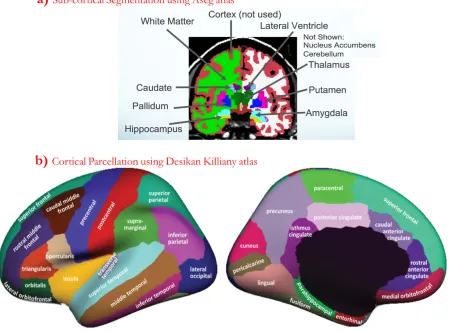
structures. At each voxel of the standard atlas, one of the 37 anatomical labels including left and

right caudate, putamen, pallidum, thalamus, lateral ventricles, hippocampus, and amygdala (see

Figure 2.5a), can belong to a voxel. The intensity distribution of each label is modeled as a

Gaussian. Local spatial relationships between the labeled brain structures are encoded by an

anisotropic non-stationary MRF. After registration to the atlas, the maximum posteriori estimate

of the segmentation or the probability of an anatomical label belonging to each voxel is calculated.

(38)

information or the probability that an anatomical label can be present at a particular voxel. This

information is derived from the atlas and the affine transformation of the input image to the atlas.

The second is the local spatial information or the local spatial relationship between anatomical

labels such as “posterior amygdala is frequently superior to anterior hippocampus, but never

inferior to it” (Fischl et al., 2002). This spatial relationship is encoded by an anisotropic

non-stationary MRF.

2.3.3.2 Cortical parcellation

FS subdivides the cerebral cortex on a brain MRI into a number of gyral based regions of

interest or parcellations (Fischl et al., 2004; Desikan et al., 2006). It utilizes the prior information

from a standard atlas such as the Desikan-Killiany atlas (Desikan et al., 2006) which was created

using a dataset of 40 MRI scans, where in each scan, 35 cortical regions were manually identified

in each of the individual hemispheres (see Figure 2.5b). The local surface geometry of a location in

the cortex and the prior information derived from the atlas are combined in a Bayesian framework

to calculate the maximum posteriori estimate of a brain parcellation belonging to that location.

Similar to sub-cortical segmentation, the prior information has two sources. The first source is the

global spatial information; it is the probability that a given parcellation occurs at a particular

location in the atlas, independent of the local surface geometry. This information is provided by

the atlas and the registration of the input image to the atlas. The second source is the local spatial

information or the local spatial relationship between parcellation labels such as “precentral gyrus

can be anterior, superior or inferior to central sulcus but never posterior to it” (Fischl et al., 2004).

(39)

[image:39.612.94.545.87.420.2]

Figure 2.5: Sub-cortical segmentation & cortical parcellation in Freesurfer (FS).

Figure a) was borrowed from http://slideplayer.com/slide/5222876 and figure b) was borrowed from Klein and Tourville (2012).

2.3.3.3 FS Features

After the segmentation of cortical and sub-cortical brain regions, different morphometric

and intensity properties or features of these regions can be calculated. Volume, intensity mean,

intensity standard deviation (std.) of 40 sub-cortical brain structures are automatically estimated by

the recon-all workflow. Similarly, recon-all automatically estimates the volume, surface area,

Gaussian curvature, mean curvature, curvature index, folding index, thickness mean, thickness

standard deviation, intensity mean, and intensity std. for the 34 cortical brain regions of each

(40)

Mean curvature is the arithmetic mean of principal curvatures !"#$%!"&'

( where K*+, and

K_*-. are maximum and minimum principal curvatures respectively. Mean curvature measures the

extrinsic curvature. Extrinsic curvature refers to the amount of folding created with no distortion.

Gaussian curvature is the square of the geometric mean of principal curvatures K_*-.K_*+,.

Gaussian curvature measures the intrinsic curvature and its sign can be used to characterize the

surface. Intrinsic curvature refers to the folding created with distortion or shearing i.e. it is

excess/deficit in the surface area compared to a plane at the point (Schaer et al., 2008).

Folding index is defined as ₀₁/ K_*+, K_*+, − K_*-. 𝑑𝐴 (VanEssen & Drury, 1997).

Folding index is an overall measure of the folding of a surface. For any sulci having the shape of a

half-cylinder, its folding index is proportional to its length.

2.4

Analysis of neuroimaging data

Neuroimaging data analysis can be mainly categorized in three groups: voxel-based,

vertex-based, and feature-based.

2.4.1

Voxel-based

In voxel-based studies, the voxel intensities are compared between the images. The analysis

is usually preceded by the registration of the brain images to a standard space to ensure

voxel-to-voxel correspondence across images by adjusting the 3D coordinates of a voxel-to-voxel to best match the

MRI intensities across subjects at that particular voxel (Greve, 2011). Image registration is

generally followed by image smoothing and the amount of smoothing or the size of the low pass

filter used for smoothing is proportional to the size of the region of interest. The intensity of a voxel

in a final smoothed image may represent intensity, volume, or concentration of a tissue class at that

(41)

Representative voxel-based neuroimaging studies include: Nishida et al. (2011) reporting larger

anterior insular volume in patients with obsessive–compulsive disorder, May (2011) demonstrating

experience-dependent structural plasticity in the adult human brain, Matsuda et al. (2012)

detecting Alzheimer’s, Walther et al. (2009) relating brain structural differences to body mass index

in older females, Demirakca et al. (2011) reporting diminished GM in the hippocampus of cannabis

users, Kühn, Schubert, and Gallinat (2010) reporting reduced thickness of medial orbitofrontal

cortex in smokers, etc.

2.4.2

Vertex-based or Surface-based

In vertex-based or surface-based studies, the surface area of a brain structure is explicitly

represented by a mesh of triangles. The point where the vertices of the neighboring triangles meet

is called a vertex. A vertex can be localized by two spherical coordinates (longitude and latitude)

on a surface. After a brain surface such as the pial surface is represented by a mesh of triangles,

several geometric features such as area, curvature, thickness, etc. can be computed. For group

analysis, the surface based registration is performed where the 2D spherical coordinate of a vertex

is adjusted to match the curvature across subjects so that the folding patterns are aligned as

described by Greve (2011). Representative vertex-based neuroimaging studies include: Tondelli et

al. (2012) reporting atrophy in the right medial temporal lobe and the right hippocampus in

Alzheimer’s patients 10 years before clinical diagnosis, Im et al. (2006) reporting cortical thickening

in women in localized anatomical regions, Zarei et al. (2010) reporting significant bilateral regional

atrophy in the dorsal-medial part of the thalamus in Alzheimer’s patients.

2.4.3

Feature-based

In feature-based studies, the different features or properties of the brain regions are

(42)

based such as the mean intensity of a brain region. The feature-based analysis is usually preceded

by the segmentation of various cortical and sub-cortical brain regions and the calculation of

different features of these regions. The feature extraction may involve many vertex and voxel based

techniques. In this thesis, all analyses are feature-based and the scope is limited to feature-based

analysis from here on.

Usually in feature-based studies, the group differences in a feature or a group of features

are investigated. When a study involves only one feature or treats each feature in a group to be

independent of each other, it is called a univariate study. A typical univariate study utilizes a

statistical model such as General Linear Model (Nelder et al., 2006) to investigate the group

differences in brain features. In contrast, when a study treats the individual features to be

dependent of each other and tries to identify a multi-variate pattern between two groups, it is called

a multi-variate study. A typical multi-variate study utilizes machine learning techniques to identify

multi-variate differences in a data-driven fashion.

2.5

Machine Learning

Machine learning is the process of learning the underlying structure of a dataset and using

that knowledge to make predictions on unseen data (Alpaydin, 2010). An algorithm or a collection

of algorithms are applied on samples of a population to learn underlying structure or study the

probability distribution of the population. Machine learning techniques capture the multi-variate

relationships in data and hence are well-suited to detect subtle and distributed differences in the

data. So, compared to univariate techniques, machine learning techniques can perform better in

capturing the brain morphology of heterogeneous conditions like ASD. Thus, they hold promise

for improving our knowledge of ASD brain morphology and identifying brain biomarkers helpful

(43)

Machine learning techniques cover three major areas: supervised learning, unsupervised

learning, and reinforcement learning.

In supervised learning a training dataset with class labels are given and the algorithm learns

the input to output mapping function or a pattern in the training data. The learned mapping

function is then used to predict the labels of an unseen test data. The inherent assumption here is

that the training and testing data are similar. In other words, the same probability function

generates both training and test data. Supervised learning can be a classification problem when

the target label is categorical, or a regression problem when the target label is continuous. Some

applications of supervised learning are stock prediction (Rather et al., 2017), mortality prediction

(Katuwal & Chen, 2016), spam detection (Chakraborty et al., 2016), cancer detection (Bazazeh &

Shubair, 2016), ASD detection (Kim et al., 2016) etc. Some examples of supervised learning

algorithms are regression models, naïve Bayes, decision trees, Random Forest (RF), Gradient

Boosting Machine (GBM), neural networks, etc.

In unsupervised learning, class label information is absent and the algorithm has to learn

the underlying structure of the data by itself. Unsupervised learning can be a goal in itself, such as

finding sub-groups or clusters in the data or can be an intermediate step such as dimensionality

reduction for subsequent machine learning steps. Some applications of unsupervised learning are

human action categorization (Niebles et al., 2008), extracting hierarchical features for object

recognition (Ranzato et al., 2007), discovery of human neural-behavioral maps (Vogelstein et al.,

2014), identifying sub-groups of ASD (Gupta, 2015), etc. Some examples of unsupervised learning

algorithms are K-means, mixture models, principal component analysis, autoencoder, and

generative adversarial networks.

In reinforcement learning, an agent or a group of agents is trained in an environment to

(44)

process (Puterman & L., 1994) with its inputs as the actions of the agent and outputs as the

observations and rewards sent to the agent. Reinforcement learning is particularly well-suited to

problems where trade-off between long-term and short-term reward is important. Some

applications of reinforcement learning are robot control (Kober et al., 2013), playing Go (Silver et

al., 2016) , and playing poker (Brown & Sandholm, 2017).

In this thesis, we applied supervised learning techniques namely RF (Breiman, 2001) and

GBM (Friedman, 2000). These two algorithms are briefly explained below.

2.5.1

Random Forest (RF)

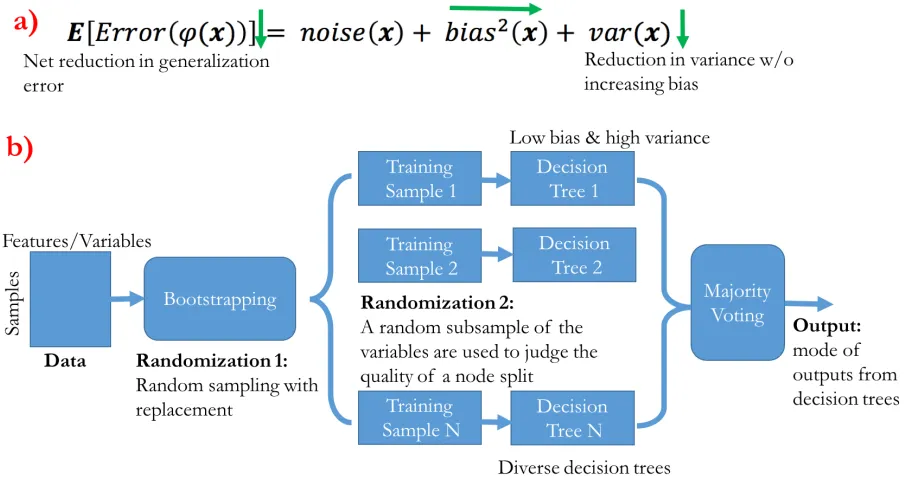
RF (Breiman, 2001) is an ensemble of decision trees and its output class is the mode value

of the output classes of the individual decision trees (see Figure 2.6). It is an ensemble technique

that relies on the reduction of the variance of the general error term. For the squared error loss,

the expected generalization error of a model φ at a given point 𝐱 can be decomposed into three

components (Gelman & Hill, 2006) as in Equation 2.1.

E Error φ(x) = noise 𝐱 + bias( _{𝐱 + var(𝐱)} _(2.1)

In Equation 2.1, the first term noise 𝐱 is the irreducible error or Bayes error. It is the

theoretical lower bound on the generalization error and is independent of both learning algorithm

and data. The second term bias( _𝐱 _{is the difference between the average prediction of the model}

and the prediction of the Bayes model. The third term var(𝐱) is the variability of the predictions

at point 𝐱 over the models learned from all possible subsets of population.

The main idea of RF is to decrease the variance term by keeping the bias constant, thereby

decreasing the overall error of the ensemble. It achieves this variance reduction by averaging the

high variance classifiers or decision tree classifiers. The more diverse or uncorrelated the decision

(45)

each other, RF introduces randomness while constructing the trees, hence the name ‘random

forest’. The randomization is introduced at first during data sampling and then while constructing

the decision trees. Each tree learns from a bootstrap replica of the data obtained by random

sampling with replacement in the original data. This introduces a degree of randomness in the

decision trees because they are trained with different bootstrap replicas. While growing decision

trees, the quality of a node split is based only on a random subsample of the variables instead of all

[image:45.612.90.545.269.511.2]

of them. Most of the randomization comes from this step.

Figure 2.6: Random Forest is an ensemble of decision trees.

a) Generalized error broken down into three terms: noise, bias, and variance. Random Forest (RF) relies on the reduction of variance without increasing bias, thus reducing the overall error. The directions of the green arrows correspond to the direction of change of the error terms due to ensembling. b) General block diagram of RF as an ensemble of diverse decision trees.

A decision tree is a simple classifier which iteratively partitions the data space into more

homogenous partitions using simple decision rules. The quality of the data partitions or the child

nodes after a node splitting in a decision tree is measured by their homogeneity. The homogeneity

(46)

(Breiman, 1996), entropy (Gray & M., 1990), etc. and the quality of the node split is quantified by

change in these metrics.

In a RF, the importance of a variable is the sum of the weighted impurity decreases in all

node splits by the variable, averaged over all trees in the forest (Breiman, 2001; Louppe, 2015). It

is calculated as in Equation 2.2.

Imp X_K = 1

M 1(jO= j) p(t)Δi(sO, t)

S"

T

*U/

(2. 2)

Where,

Imp XK = the importance of variable XK

jO = the identifier of the variable used for splitting node t

s_O = a split at node t due to variable X_K

p t = the proportion XY

X of samples at node t where NOis the number of samples at node t and N is the total number of samples

Δi s_O, t = decrease in node impurity by split s_O

φ_* = mth _decision_tree

M = the number of decision trees in the forest

In this thesis, RF was used as the first choice classifier since it is inherently suitable for

parallel processing, has very few hyper parameters to tune, does not require data scaling, is

theoretically resistant to overfitting, provides variable importance, and has been found to be very

good for a variety of datasets (Breiman, 2001; Caruana & Niculescu-Mizil, 2006).

2.5.2

Gradient Boosting Machine (GBM)

Boosting is an ensemble technique that relies on bias reduction to reduce the generalized

(47)

several weak or base learners with high bias and low variance such as decision tree stumps into one

strong learner. The base learners are combined so that the ensemble bias decreases while variance

remains the same, thereby reducing the net ensemble error. At each iteration or boosting step,

GBM constructs a new base learner to be the most parallel to the negative gradient of a loss

function along the observed data so that the new base learner focuses on the weakness of the model

(Natekin & Knoll, 2013). In other words, it performs functional approximation of a model by

consecutively improving along the negative direction of a loss function. In this thesis, a binomial

(48)

3

CHAPTER

3:

DEPENDENCY

OF

BRAIN

FINDINGS ON IMAGE PROCESSING TOOLS

AND POTENTIAL SOLUTIONS

Some material from (Katuwal et al., 2016b) has been reused in this chapter under Creative Commons Attribution

(CC BY) license.

Previous studies applying automatic brain image processing methods on MRI report

inconsistent neuroanatomical alterations in ASD. In this study, we investigate methodological

differences as a possible cause behind these inconsistent findings. In particular, we focus on the

estimation of the following brain volumes: GM, WM, CSF, and TIV. T1-weighted MRIs of 417

ASD subjects and 459 TDC from the ABIDE dataset were estimated using three popular

preprocessing methods: SPM, FSL, and FS. The estimated brain volumes were correlated but had

significant inter-method biases. ASD vs. TDC differences in all brain volume estimates were highly

dependent on the method used. When methods were compared with each other, they showed

differential biases for ASD, and several biases were larger than ASD vs. TDC differences of the

respective methods. After manual inspection, we found inter-method segmentation mismatches in

the cerebellum, sub-cortical structures, and inter-sulcal CSF. In summary, method dependent ASD

vs. TDC differences indicate that the inter-method discrepancy can contribute to inconsistent

neuroimaging findings in ASD. We suggest cross-validation across methods and emphasize the

need to develop better methods to increase the robustness of neuroimaging findings.

(49)

MRI is a powerful tool used to investigate the human brain in vivo and to find associations

between brain morphometry and brain disorders. Although a large number of MRI studies have

been conducted, consistent MRI markers for brain disorders are yet to be found (Chen et al. 2011).

This can mainly be attributed to low statistical power of neuroimaging and neuroscience studies

(Button et al., 2013). Inconsistent results may be due to differences in the demographics of data

(Stanfield et al., 2008), image acquisition settings (Auzias et al., 2014a; Styner et al., 2002),

assumptions made on data and algorithms used (Eggert et al., 2012; Fellhauer et al., 2015;

Nordenskjöld et al., 2013), and even machines used to process the data (Gronenschild et al., 2012).

With the increasing use of automated preprocessing methods in neuroimaging studies, the

effect of inter-method variations in neuroimaging findings merit an investigation. Although

automatic methods are more objective than manual methods, they possess method-specific bias

and variance (Eggert et al., 2012; Nordenskjöld et al., 2013). The bias and variance across methods

arise mainly due to method specific assumptions made on data, varying definition of brain

structures, different image processing algorithms, varying sensitivity to imaging artifacts such as

motion, and use of inconsistent a priori information such as brain templates. A number of previous

studies have reported significant inter-method inconsistencies (Eggert et al., 2012; Fellhauer et al.,

2015; Hansen et al., 2015; Ren et al., 2005; Tsang et al., 2008). Eggert et al. (2012) reported

pronounced differences (11%) in mean segmented GM volumes from four standard segmentation

algorithms: SPM8 New Segment, SPM8 VBM, FSL v. 4.1.6 and FS v. 4.5. According to Hansen et

al. (2015), compared to manual segmentation, FS 4.5 underestimated TIV by 7 %. Similarly,

differences in segmentation accuracies between FSL and SPM5 were reported by Tsang et al.

(2008).

One important concern is that inconsistent results driven by inter-method variations can

(50)

Several previous studies have shown that the magnitude and even the direction of the effect size

can be dependent on the method used. Boekel et al. (2015) performed a replication study on 17

brain structure-behavior correlations from five neuroimaging studies and were not able to replicate

any of the correlations. A response paper by Muhlert and Ridgway (2015) pointed out that one of

the reason the correlations could not be replicated is the methodological differences between SPM

and FSL. Nordenskjöld et al. (2013), compared SPM8 and FS v. 5.1.0 TIV estimates to reference

TIV obtained from manual segmentation of proton density weighted images. They report that

both SPM8 and FS overestimated TIV. In addition, SPM showed systematic bias associated with

gender (systematic overestimation of TIV in females) and aging atrophy while FS showed bias for

reference TIV (systematic overestimation of TIV for larger skull size). Notably, hippocampal

volume showed different associations with education depending on which TIV measure (SPM or

FS) was used for hippocampal volume normalization. When normalized with SPM TIV, there was

no association between hippocampal volume and education, whereas when normalized with FS

TI

Machine Learning Based Autism Detection Using Brain Imaging

Rochester Institute of Technology

RIT Scholar Works

Machine Learning

Rochester Institute of Technology

ACKNOWLEDGMENTS

ABSTRACT

ABBREVIATIONS

CONTENTS

CHAPTER 1: INTRODUCTION ... 1

2 CHAPTER 2: BACKGROUND ... 12

4 CHAPTER 4: UTILIZING NON-BRAIN INFORMATION TO IMPROVE ASD DETECTION BASED ON BRAIN MORPHOLOGY ... 62

5 CHAPTER 5: EARLY DETECTION OF AUTISM USING BRAIN MORPHOLOGY .... 94

CHAPTER 6: CONCLUSION AND FUTURE WORK ... 120

BIBLIOGRAPHY ... 126

FIGURES

TABLES

CHAPTER 1: INTRODUCTION

Importance of early detection of ASD

Problem 1: Behavior based diagnosis of ASD is late and does not help

Problem 2: Inconsistent brain anatomical findings in ASD

Problem 3: Low Classification success in large multi-site data

Demonstrating MRI as a potential tool for detection

Relating inconsistent findings and low classification success to ASD

Providing the evidence of brain image processing tool dependent findings and

Divide and Conquer: we propose identifying brain biomarkers in sub-groups of

Brain biomarkers discovery for early detection of ASD

Thesis Organization

Chapter 2: Background

Chapter 3: Method Dependent Findings

Chapter 4: Brain Morphology Based ASD Detection and Tackling ASD

Chapter 5: Early Detection of ASD

Chapter 6: Conclusion

Brain Imaging

MRI acquisition

Brain Feature extraction from MRI

Analysis of neuroimaging data

Vertex-based or Surface-based

Feature-based

Machine Learning

Random Forest (RF)

Gradient Boosting Machine (GBM)

CHAPTER