Curvature-related eddy-current losses in laminated axial flux machine cores

Curvature related Eddy current losses in laminated

Axial flux machine cores.

A. Ahfock and A. J. Hewitt MIEE.

Abstract — In this paper we present an axiperiodic quasi-static model to evaluate the magnetic flux density distribution and power loss due to curvature related radial

flux in the laminated core of axial flux machines. It is shown that the relatively low

effective permeability in the radial direction and the shielding effect of induced eddy

currents result in negligible radial flux density compared to the peak flux densities in

the axial and circumferential directions. This justifies the assumption of zero radial

flux which simplifies electromagnetic modelling of axial flux machine cores. The

model predicts that power loss due to curvature related radial flux is insignificant

compared to normal eddy current loss if the core permeability, core conductivity and

number of poles are sufficiently high. A laboratory technique is proposed for the

practical detection of power loss due to curvature related radial flux.

NOMENCLATURE

B = magnetic flux density D = power loss density E = electric field intensity

F = loss due to cross-lamination flux

f = frequency

H = magnetic field intensity

I = vector of induced currents

J = induced current density L = core axial length

P = matrix of permeances

P = total core loss

p = number of machine poles

Q = matrix of permeances

R = matrix of resistances

Ri = core inner radius

Ro = core outer radius

S = matrix of permeances

T = electric vector potential

W = matrix of permeances

δ = skin depth

µ = material permeability

σ = material conductivity

Φ = vector of imposed magnetic flux

Ω = vector of magnetic scalar potentials

I. INTRODUCTION

Axial flux machines (AFMs), because of their physical structure, have an advantage

in applications such as fans, disk drives and some electric vehicles. It has also been

suggested [1,2,3] that, compared to radial flux machines they have greater power to

weight ratios.

It is important for those who design AFMs to have a good understanding of the

magnetic flux density distribution in those machines. There have been a number of

publications [2,4,5] on the flux density distribution in the air-gap of AFMs. However,

they effectively ignore the flux density distribution in the iron cores since infinite

permeability is assumed. In this paper the focus is on the flux distribution in the

laminated cores of AFMs taking into consideration the curvature of the core. The aim

is to determine the practical significance of any curvature related radial component of

flux density that may be present in the core. Boldea, Rahman and Nasar [6] derive

expressions for the flux density in machine cores, but they ignore the effects of

curvature. Hewitt, Ahfock and Suslov [7] concluded that curvature related radial flux

density is relatively small compared to the peak axial and circumferential flux

densities even when the shielding effect of induced eddy currents is ignored. Their

model is a magnetostatic one and thus did not address the question of power loss

resulting from curvature related radial flux. In this paper a quasi-static

electromagnetic model is used to confirm the findings of [7] and to evaluate power

loss due to curvature related radial or cross-lamination flux. The model is specifically

for cores in which the flux enters axially from the air-gap(s) and then travels

In Section II it is shown that power loss due to cross-lamination flux is decoupled

from power loss due to parallel running flux. Therefore, their theoretical evaluations

can be done separately. Sections III, IV, and V are devoted to the development of an

electromagnetic model for the core that is used in Sections VI and VII for the

prediction of flux density distribution and power loss, respectively. In Section VIII a

closed form expression for power loss is derived. Although this expression is not as

accurate as the more detailed electromagnetic model developed Sections III, IV and

V, it allows a quick assessment to be made on the relative importance of curvature

related power loss. Section IX is about laboratory tests for the practical detection of

power loss due to curvature related radial flux and Section X concludes the paper.

II. EDDY CURRENT LOSS SEPARATION

Induced currents within a lamination sheet are made up of the superposition of eddy

currents due to flux that runs parallel to the lamination faces and eddy currents due to

cross-lamination flux. Assume that the distribution of eddy currents due solely to a

given distribution of parallel running flux is given by X. Similarly, assume that the

distribution of eddy currents due solely to a given distribution of cross-lamination flux

is given by Y. We now show that the power loss due to eddy current distribution X

and that due to eddy current distribution Y are mutually independent and that

interaction between the two eddy current distributions contribute zero net additional

power loss. The power loss density, D, at any given point within a laminate is given

by:

(

) (

)

2

c p zc zp

rp

r z

J J J J J

D θ θ

θ

σ σ σ

+ +

where the subscripts r, θ and zdenote the radial, circumferential and axial

directions, respectively, subscripts pand crelate to parallel running flux and

cross-lamination flux, respectively, σ is the material conductivity and Jis the induced

current density.

Expansion of the right hand side of equation (1) gives:

2 2 2 2 2 _{2 2}

rp p zp c zc c p zc zp

r z z z

J J J J J J J J J

D θ θ θ θ

θ θ θ

σ σ σ σ σ σ σ

= + + + + + + (2)

The first three terms of equation (2) represent contributions to power loss density

coming from parallel running flux alone. The fourth and fifth terms represent

contributions to power loss density coming from cross-lamination flux alone. The last

two terms represent contributions to power loss density which result from the

interaction between the two sets of induced currents. The following assumptions are

now made:

a) J_θc and J_zc are constant along a radial line within a laminate; and

b) If x is measured radially from the laminate centre, as shown in Figure 1, then,

( )

p

J_θ x is equal to −Jθp

( )

( )

( )

Based on these assumptions, it is clear that the last two terms in equation (2) do not

contribute to the total power loss in the lamination.

The decoupling between power loss due to the parallel running flux and that due to

cross-lamination flux allows them to be calculated separately. There are well

established methods for the calculation of power loss due to parallel running flux [8]

and these are applicable to laminated cores of axial flux machines. In this paper we

and parallel running flux are both present in the adopted model, eddy currents due to

the latter have been eliminated by assuming zero radial conductivity. Whilst this

assumption makes power loss due to parallel running flux equal to zero, it has no

effect on the power loss due to cross-lamination flux.

III. PROBLEM FORMULATION

The following simplifying assumptions are made:

a) Magnetic saturation and hysteresis are negligible.

b) Induced eddy currents do not have a radial component.

c) Permeabilities in the radial, axial and circumferential directions may differ, but

are constants.

d) The core is considered solid rather laminated. However a much lower radial

permeability is used to account for the lower permeability of the electrical

insulation between laminations [9].

e) The core surface on the air-gap side is smooth, that is the effects of teeth and slots

are ignored.

f) Flux enters the core from the air-gap side axially, with a sinusoidal variation in the

circumferential direction.

g) The regions outside the core have zero permeability.

h) The quasi-static approximation to Maxwell's equations is applicable.

Based on assumption h) we can write:

0 B

∇ ⋅ =r (3)

H J

∇× r = r (4)

B E

t

∂ ∇× = −

∂

r r

0 J

∇ ⋅ =r (6)

where Bris the magnetic flux density, Hrthe magnetic field intensity, Erthe electric

field intensity and Jris the current density.

The assumed constitutive relationships for the core are:

Br =µHr (7)

and

Jr=σEr, (8)

where 0 0 0 0 0 0 r z θ µ µ µ µ ⎡ ⎤ ⎢ ⎥ = ⎢ ⎥ ⎢ ⎥ ⎣ ⎦

, (9)

and

0 0 0

0 0

0 0 z

θ σ σ σ ⎡ ⎤ ⎢ ⎥ = ⎢ ⎥ ⎢ ⎥ ⎣ ⎦

. (10)

We have chosen to adopt the T− Ω formulation [10]. The solenoidal condition of

equation (6) allows Jrto be defined by

Jr= ∇×Tr (11)

where Tris the electric vector potential. Combining equations (4) and (11) we have

(

)

∇× r − r = . (12)

Equation (12) allows

(

)

(

)

where Ωis the magnetic scalar potential. From equations (3), (7) and (13) we get

0

T

µ µ

∇ ⋅ r− ∇ ⋅ ∇Ω = . (14)

(

)

1

T j T

σ− ωµ

∇× ∇× = −r r− ∇Ω (15)

where the time derivative has been replaced by the jωoperator since analysis is

restricted to the sinusoidal case at steady-state.

Assumption b) implies that Jrdoes not have any radial component and thus the axial

and circumferential components of the vector Trcan be chosen to be zero.

Substituting equation (9) into (14) and expanding gives

2 2 2

2 2 2 2 0.

r

r z r r

T T

r r r r z r r

θ

µ µ

µ µ µ µ

θ

∂ Ω ∂Ω ∂ Ω ∂ Ω ∂

+ + + − − =

∂ ∂ ∂ ∂ ∂ (16)

By equating the radial components on the left and right hand sides of equation (15)

and substituting equations (9) and (10) we obtain

2 2

2 2 2

1 1

0

r r

z

T T

j j T

r r _θ z

ωµ ωµ

σ θ σ

∂Ω_{− +} ∂ ₊ ∂ ₌

∂ ∂ ∂ . (17)

It is possible to obtain another two equations by equating the circumferential and axial

components of equation (15), respectively, however this is not necessary as there are

only the two unknowns T and Ω. These two unknowns will be fully defined through

equations (16), (17) and the imposed boundary conditions.

We now simplify equations (16) and (17) using the periodicity condition of

assumption f). The sinusoidal variation in the imposed magnetic flux density at the

core surface will result is the same behaviour for both Tand Ω. Therefore:

2 2

2 ₂

p

θ

∂ Ω_{= −}⎛ ⎞ _Ω

⎜ ⎟

∂ ⎝ ⎠ (18)

2 2 2 ₂ T p T θ ∂ ⎛ ⎞ = −⎜ ⎟

∂ ⎝ ⎠ , (19)

(16) results in

2

2 2

2 2 ₂ 2 0

r r

r z r

p T

T

r r r r z r r

θ

µ

µ µ

µ ∂ Ω+ ∂Ω− ⎛ ⎞_{⎜ ⎟} Ω +µ ∂ Ω−µ ∂ − =

∂ ∂ ⎝ ⎠ ∂ ∂ (20)

and substituting equation (19) into (17) gives

2 ₂ 2 2 1 1 0 2 r r z p T

j j T T

r r _θ z

ωµ ωµ

σ σ

∂Ω_{− −} ⎛ ⎞ ₊ ∂ ₌

⎜ ⎟

∂ ⎝ ⎠ ∂ (21)

Based on assumptions f) and g) the imposed boundary conditions are such that the

normal derivative of Ω is zero at all surfaces except at the air-gap boundary where

( )

∂Ω₌ ⎛ ⎞

⎜ ⎟

∂ _{⎝ ⎠}. (22)

It is now possible to solve for Tand Ω using equations (20) , (21) and the imposed

boundary conditions. From the solution, the power loss due to induced eddy currents

can be found.

IV. NUMERICAL SOLUTION

In principle any numerical technique could be used to solve for the fields inside the

core. An attempt was made to solve the full 3D problem on a PC using commercially

available finite element software. This was without success because of memory

requirements. By taking advantage of the problem periodicity in the circumferential

direction (see equations (18) and (19)) the problem can be reduced to one that is

effectively two dimensional. The axiperiodic formulation is however not commonly

specifically written to solve this problem. The finite difference method was chosen

because of its suitability and simplicity when the problem's geometry is simple.

The core is discretised as shown in Figure 2. The discretised plane is chosen to be a

pole centre plane along which the angular coordinate θ is equal to zero. The plane

contains e_r×e_z elements, where e_ris the number of divisions in the radial direction

and e_zthe number of divisions in the axial direction. An element centred at radius r_i,

has a volume given by ∆ ∆r z r di θ where dθ is infinitely small. A node is assumed to

exist at the centroid of each element. The location of a node is identified by three

subscripts i, j and k which increment in the positive radial, circumferential and

axial directions, respectively. Node

(

)

(

)

node location index jand explicit reference to the dimension dθ of the elements are

not essential, but are included for ease of physical interpretation. Subscripts i, j, k

when used with Ω and T indicate values of those quantities at node

(

)

discretised form of equations (20) and (21) are derived in Appendix A. Application of

those at all nodes results in the following matrix equation:

jω jω

⎡ ⎤ ⎡ ⎤ ⎡ ⎤

=

⎢ ₊ ⎥ ⎢ ⎥ ⎢ ⎥

⎣ ⎦ ⎣ ⎦ ⎣ ⎦

P Q Ω Φ

W R S I 0 (23)

where Pis an

(

) (

)

(

) (

(

)

)

of permeances, Wis an

(

(

)

)

(

)

(

)

(

)

(

(

)

)

(

(

)

)

(

(

)

)

through to node

(

)

(

(

)

)

an

(

)

(

)

, , ₂

i j k i j k i j k

T T r

I = + + ∆ . (24)

Current I_{i j k, ,} is effectively a loop current that exists around a reluctive branch between

nodes

(

)

(

)

direction restricts the existence of those loop currents around radial reluctive branches

only.

Expressions for the evaluation of entries for P, Q, W, R and S are derived in the

appendix in terms of physical dimensions and material properties. The appendix also

provides expressions for the elements of Ф in terms of the imposed boundary

conditions. Values for vectors Ωand Iare found by solving equation (23). From these

values the magnetic flux density at any point in the core and the power loss due to

induced currents can be evaluated.

V. POWER LOSS CALCULATION

In terms of the electric vector potential, power loss density D is given by

2 2

2

1 1

z

T T

D

z r

θ

σ σ θ

∂ ∂

⎛ ⎞ ⎛ ⎞

= _{⎜ ⎟} + _{⎜ ⎟}

∂ ∂

⎝ ⎠ ⎝ ⎠ . (25)

For the axiperiodic case

( )

ˆ , cos 2

p T =T r z ⎛_⎜ θ ⎞_⎟

⎝ ⎠ (26)

where T r zˆ ,

( )

2 ₂

2 2 2

2

ˆ

1 1 _ˆ

cos sin

2 z 2

T p p

D T z r θ θ _θ σ σ ⎛∂ ⎞ ⎛ ⎞ ⎛ ⎞ = _{⎜ ⎟ ⎜ ⎟}+ _{⎜ ⎟} ∂ _{⎝ ⎠ ⎝ ⎠}

⎝ ⎠ . (27)

Equation (24) allows Twithin the half of any element between r_i and r_i+ ∆r 2 to be

approximated as Ii j k_{, ,} ∆r, and similarly, in the other half T can be approximated as

1, ,

i j k

I₋ ∆r.

Based on the above arguments, we arrive at equation (28) which is an expression for

the core power loss, F, due to the induced currents.

(

)

(

) (

)

2

, , 1, , , , 1 , , 1 1, , 1 1, , 1 1 1

2 2 2 4

r z

e e

i j k i j k i j k i j k i j k i j k

i

i k z i

I I z I I I I

p

F r

r r _θ z r

π σ σ − + − − + − − = = ⎡ ⎤ + ∆ − + − ⎛ ⎞ _{⎢ ⎥} = _{⎜ ⎟} + ⎢ ⎥ ∆ ∆ ∆ ⎝ ⎠ _{⎣ ⎦}

∑∑

1, , 1, , 1 1, , 1 , , , , 1 , , 1 , , 1 1, , 1 , , 1 1, , 1

1

0 if 0

0 if

0 if 1

0 if

i j k i j k i j k

i j k i j k i j k r

i j k i j k

i j k i j k z

j

I I I i

I I I i e

I I k

I I k e

− − + − − + − − − − + − + = = = = = = = = = = = = = = =

and all other values of I are obtained by solving equation (23).

The above expression for power loss is for the case where the fields are stationary

with respect to the core and pulsating at frequency ω. That is B r

(

)

(22) is given by B rˆ_z

( ) ( ) (

)

(

)

( ) (

)

z z

It can be shown that, for any given B rˆz

( )

twice that for the pulsating field.

VI. THEORETICAL PREDICTION:FLUX DENSITY DISTRIBUTION

The model developed in Sections III, IV and V has been used to analyse the flux

density distribution in a core with the following nominal characteristics: R_i =0.075m,

0.175m o

R = , L=

(

)

6

5 10 S/m

θ

σ = × , _{5 10 S/m}6

z

σ = × , ω =100π and Bˆ_z =0.7 T. In practice it would be

expected that the core back-iron length L will be progressively reduced as the number

of poles is increased. For this reason the length of the back-iron has been chosen be

inversely proportional to the number of poles. Figure 3 shows theoretical predictions

for the normalised radial flux density as a function of radius, and averaged over the

core axial length. Similarly, Figure 4 shows the normalised circumferential flux

density as a function of radius, averaged over the core axial length.

The following observations can be made:

a) The peak radial flux density is much smaller than the peak axial or circumferential

flux densities.

b) The radial flux density is almost non-existent under a.c. conditions. This is

theoretical confirmation of what was already postulated in reference [7] based on

magnetostatic analysis and experimental results.

c) The amount of radial flux, although small, is a strong function of core

d) The circumferential flux density is greatest near the outer radius of the core. As

stated in [7], this must be accounted for when sizing the back-iron of axial flux

machines.

VII. THEORETICAL PREDICTION:POWER LOSS

The core model has also been used to make predictions of power loss due to

cross-lamination flux. The assumed nominal core characteristics are the same as those of

Section VI. Power loss predictions are shown in Table 1 and Figure 5.

For comparison, classical eddy-current power losses due to parallel flux, Fp, have

been evaluated using

equation (30) [8].

(

)

2 2 ₂

, , 24

p

V

t

F =ω σ

∫

where tis the laminate thickness (= 0.27mm) and V the core volume. These values

are shown in Table 2.

The following observations can be made:

a) There is a strong dependence of power loss Fon the number of poles and on the

relative permeability of the core.

b) Except for the two-pole case and at low values of core permeability, the power

loss due to cross-lamination flux is insignificant compared to the power loss due to parallel flux.

c) The power loss due to cross-lamination flux may be expressed as:

F=k f (31)

where kis independent of frequency but is a function of physical dimensions,

are obtained with kchosen to be 0.2285 and 0.0691 for the 2- and 4- pole cases,

respectively.

The explanation for observation c) is based on characteristics of the circumferential

component of the induced current which is shown in Figures 6 and 7. The first point is

that the induced current experiences high resistance circumferentially since it is

restricted to flow through a thin layer near the flat surfaces of the core because of the

skin-effect. The second point is that the total circumferential current (Figure 7) is

practically independent of frequency. The high circumferential resistance, compared

to the axial resistance, implies that practically all the power losses are associated with

the circumferential component of current. Thus we have a current, which is itself

almost independent of frequency, flowing through a cross-sectional area that is

proportional to the skin-depth. This implies that the power loss is proportional to the

square root of frequency.

VIII. CLOSED FORM EXPRESSION FOR POWER LOSS

It was shown in Section VII that the relative significance of power loss due to cross

lamination flux depends on several factors including the number of poles, material

properties physical dimensions and operating frequency. The closed form expression ,

which is now derived, can be used by axial flux machine designers to make quick

assessments on the requirement to consider power loss due to cross lamination flux.

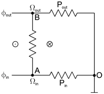
As shown in Figure 8, the core is represented by a simplified equivalent coupled

reluctive-resistive network. The reluctive circuit contains only three nodes. Nodes A

(

)

(

)

uniform magnetic potential which is equidistant from adjacent pole centre planes. The

resistive circuit is a single loop linking the reluctive branch which represents

permeance in the radial direction between nodes A and B. The following assumptions

are made:

a) Half of the flux per pole that enters the core from the air-gap between

(

)

i o i

r=R + R −R and r=R_oflows through branch BO. This is represented by

out

φ in Figure 8.

b) Half of the flux per pole that enters the core from the air-gap between r=R_i and

(

)

i o i

r=R + R −R flows through branch AO. This is represented by φ_inin Figure

8.

c) The resistance of the resistive loop is sufficiently small such that the induced

current cause the net flux flowing in the reluctive branch between nodes A and B to be practically zero.

d) Reluctance in the axial direction is assumed to be zero.

e) Branch BO represents flux paths between r=R_i+

(

)

f) Branch AOrepresents flux paths between r=R_i and r=R_i+

(

)

g) Due to the skin effect, the circumferential component of the loop current decays

exponentially from the core flat surfaces with characteristic decay length equal to the skin depth.

Equations (32) to (40) are based on the above assumptions.

(

)

(

)

p L R R P R R θ µ π − = + (32)

(

)

(

)

(

)(

)

out

ˆ 3 4

z o i o i

B R R R R p

φ = + − (34)

(

)(

)

in

ˆ 3 4

z i o o i

B R R R R p

φ = + − (35)

(

)

z

z o i

pL R R R σ π = − (36)

where R_zis the axial component of the loop resistance,

(

)

(

)

p R R

θ θ π σ δ + = − (37)

where R_θ is the circumferential component of the loop resistance and δis the skin

depth given by

2 r θ δ ωµ σ = (38)

(

)

z o i

I

P P

B R R

Lp θ φ φ π µ =

= Ω − Ω

= − − = (39)

(

)

(

)

(

)

2 2 3

2

ˆ ₂

z

z o i o i

z

F pI R R

B R R _{pL R R}

L p p

θ

θ θ

π _π

µ πσ δσ

= + ⎡ ⎤ − ₊ = ⎢ + ⎥ ⎢ ⎥ ⎣ ⎦ (40)

Table 3 compares predictions based on the axiperiodic model with those found using

equation (40). It shows that equation (40) tends to over estimate power loss by up to a

factor of 2. This is still reasonable since equation (40) is based on fairly crude

assumptions. The nature of those assumptions is such that they lead to an

very accurate, it can still be used by machine designers to allow a quick decision to be

made on whether or not there is a need for detailed investigation into power loss due

cross-lamination flux.

IX. LABORATORY TESTS

The theory that has been presented points to the possibility of increased core loss due

to the curvature of the core in axial flux machines. Curvature related loss cannot be

separately measured as it is part of the total input power to the machine. Its extraction

from total measured core loss could, however, be based on its relationship with

frequency. Total core loss, P_T, could be expressed as

3 2 2

1 2 3

T

P = +F k f +k f +k f (41)

where Frepresents loss due to cross-lamination flux, k f₁ represents hysteresis loss,

3 2 2

k f represents excess loss [11][12] and k f₃ 2represents classical eddy-current loss

due to parallel running flux.

As shown in Figure 9, if there is a significant amount of eddy current loss due to

cross-lamination flux, then the axiperiodic model predicts a non-linear relationship

between /P_T f and f . The non-linearity is characterised by a minimum point

occurring at frequency fm. The more significant the loss due to cross-lamination flux

is, compared to normal eddy current loss, the higher the value of f_m and the easier it

would be to locate using test data. The practical identification of the turning point at

m

f requires tests to be performed over a frequency range extending sufficiently below

m

f . Indication of the existence of a turning point by test data signifies the presence of

shown that if F is equal to zero, no turning point exists in the PT / f against f graph.

Equation (42) which is obtained from equations (31) and (41), is now used to show

how loss due to cross-lamination flux can be separated from the other core loss

components.

1 2 3

T

P k

k k f k f

f = f + + + (42)

By differentiating the right hand side of (42) and equating to zero we obtain

3 2 2 m 2 3 m

k =k f + k f . (43)

It can also be shown that:

(

)

(

)

(

)

2 3 2 2

2 1

m n m m

f Q Q k f k

− + −

=

− (44)

where Q_mand Q_nare defined in Figure 9. Equation (44) allows k to be estimated from

experimental data. If accurate estimation of k₂ is not possible, and it is assumed to be

zero (k₃ assuming its maximum possible value), equation (44) returns the lower

bound for k. Equation (45), which is based on the assumption of k₃being equal to zero

(k₂ assuming its maximum possible value), gives the upper bound for k.

(

)

(

)

2

3 2 2

m n m

f Q Q

k = −

− (45)

By comparing equations (44) and (45), it can be deduced that the maximum error

from assuming a zero value for k₂ in equation (44) is 41%. However, such a high

error is unlikely in practice as classical eddy-current loss will always be relatively

Figure 11 shows experimental data for test cores with the same physical dimensions

as those given in Section VI. The experimental set-up is shown in Figure 10. Core

loss, for both cores, was obtained by subtracting copper loss from the measured

power. The experimental results suggest that core loss due to cross-lamination flux is

not significant. That is, there is no indication of the existence of a turning point as test

frequency falls. From measurements made with one of the cores wound as a toroidal

transformer, the core permeability was estimated to be greater than 5000µ_o. From the

manufacturer's data σ_θ was estimated to be about _{4.5 10×} 6_{S/m. Based on these values}

the axiperiodic model predicts the losses due to cross-lamination flux to be 0.311W at

50Hz. This is relatively small compared to the total measured core loss of

approximately 21W of which 10W is estimated to be hysteresis loss. It is not

surprising, therefore, that the experimental data points in Figure 11 do not indicate the

existence of a significant amount of power loss due to cross-lamination flux.

X. CONCLUSIONS

A model has been developed to evaluate the effect of curvature on flux density

distribution and power loss in laminated cores of axial flux machines. It has been

found that, compared to the peak flux density in the axial or circumferential direction,

the flux density in the radial direction is negligible. Consequently the circumferential

flux density in the back-iron, averaged over the axial length, is proportional to radius.

Laminations near the outer radius are subject to higher circumferential flux densities

compared to laminations near the inner radius. Designers should take this into

The tendency for flux to flow in the radial direction creates an additional component

of power loss due to eddy currents. The significance of this component is strongly

dependent on the number of poles, core permeability and core conductivity. It has

been found that if the core permeability, core conductivity and number of poles are

high enough

(

)

o p

µ > µ σ > > then power loss due to curvature related

cross-lamination flux is negligible compared to normal eddy current losses. A closed

form expression has been derived to help machine designers make a quick assessment

on whether or not power losses due curvature related radial flux is likely to be

significant. If that is the case, the more detailed axiperiodic model presented here can

be used to predict the losses. Direct measurement of this power loss is not possible.

However, if values of total core loss are obtainable from tests, then, the component of

power loss due cross-lamination flux can be isolated based on its frequency

REFERENCES

[1] Varga, J. S.: 'Magnetic and Dimensional Properties of Axial Induction Motors',

IEEE Trans. Energy Convers., June 1986, EC-1, (2), pp. 137-144.

[2] Chan, C. C.: 'Axial-Field Electrical Machines – Design and Applications', IEEE

Trans. Energy Convers., June 1987, EC-2, (2), pp. 294-300.

[3] Zhang, Z., Profumo, F., and Tenconi, A.: 'Axial-flux versus radial-flux

permanent-magnet motors', Electromotion, 1996, 3, pp. 134-140.

[4] Zhilichev, Y. N.: 'Three-Dimensional Analytic Model of Permanent Magnet Axial

Flux Machine', IEEE Trans. Mag., Nov. 1998, 34, (6), pp. 3897-3901.

[5] Bumby, J. R., Martin, R. , Mueller, M. A. , Spooner, E. , Brown, N. L. and

Chalmers, B. J.: 'Electromagnetic design of axial-flux permanent magnet

machines', IEE Proc., Electr. Power Appl., March. 2004, 151, (2), pp. 151-160.

[6] Boldea, I., Rahman, A., and Nasar, S. A.: 'Finite-Width, Finite-Thickness, and

Saturation Effects in Solid-Rotor Induction Machines', IEEE Trans. Power Appar.

Syst., Sept.-Oct. 1975, PAS-94, (5), pp. 1500-1507.

[7] Hewitt, A. J., Ahfock, T., and Suslov, S. A.: 'Magnetic Flux Density Distribution

in Axial Flux Machine Cores', IEE Proc. Electr. Power Appl., March 2005, 152,

(2), pp. 292-296.

[8] Lammeraner, J., and Stafl, M.: 'Eddy currents' (ILIFFE Books Ltd., London,

1966)

[9] Reece, A. B. J., and Preston, T. W.: 'Finite Element Methods in Electrical Power

Engineering' (Oxford University Press Inc., New York, 2000)

[10] Ratnajeevan S., and Hoole H. (Editors), 'Finite Elements, Electromagnetics

[11] Barbisio, E., Fiorillo, F., and Ragusa, C.: 'Predicting Loss in Magnetic Steels

Under Arbitrary Induction Waveform and with Minor Hysteresis Loops' IEEE

Trans. Mag., July 2004, 40, (4), pp. 1810-1819.

[12] Fiorillo F., and Novikov, A.: 'An Improved Approach to Power Losses in

Magnetic Laminations under Nonsinusoidal Induction Waveform' IEEE Trans.

APPENDIX A

The purpose of this appendix is to derive expressions to evaluate the entries for matrices P, Q, W, R, S and Ф.

For each node

(

)

(

)

(

)

(

)

(

)

(

)

(

)

, , 1, , 1, , 1 2

, , 1, , , , , , 1 , , 1

2

2

1, , , , , ,

2

2 2 2

2 2 2 2 0. 2 2

i j k i j k i i i j k i i

r

i j k i j k i i j k i j k i j k

z r

i

i j k i j k i i j k

r

i i

r r r r r r

r

T T r r

z r r

T T r r p

r r r

θ µ µ µ µ µ − + + + − + −

⎡ Ω − Ω − ∆ − Ω + ∆ ⎤

⎢ _∆ ⎥

⎣ ⎦

+ + ∆

Ω − Ω − Ω

⎡ ⎤ + _{⎢ ⎥}+ ∆ ∆ ⎣ ⎦ + − ∆ Ω ⎛ ⎞ + _{⎜ ⎟} − = ∆ ⎝ ⎠ (A1)

For each node

(

)

(

)

(

)

(

)

(

)

(

)

(

)

( )

, , 1, , 1, , 1 2

, , 1, , , , , , 1

2

2

1, , , , , ,

2

2 2 2

2 2 ˆ 2 . 2 2

i j k i j k i i i j k i i

r

i j k i j k i i j k i j k

z r

i

i j k i j k i

i j k z i

r

i i

r r r r r r

r

T T r r

z r r

T T r r B r p

r r r z

θ µ µ µ µ µ − + + + + −

⎡ Ω − Ω − ∆ − Ω + ∆ ⎤

⎢ _∆ ⎥

⎣ ⎦

+ + ∆

Ω − Ω

⎡ ⎤ + _{⎢ ⎥}+ ∆ ∆ ⎣ ⎦ + − ∆ Ω ⎛ ⎞ + _{⎜ ⎟} − = ∆ ∆ ⎝ ⎠ (A2)

Application of equations (A1) and (A2) to all nodes results in the following matrix

equation

+ =

PΩ QI Φ. (A3)

(

)

P m n is non-zero only if mis equal to nor if nodes m and n are adjacent to each

other. If node n is adjacent to node m in the axial direction then

(

)

(

)

P m n P n m

z

µ ∆

= = −

∆ . (A4)

(

)

P m n dθ

− could be regarded as the permeance in the axial direction across adjacent

min the radial direction, then

(

)

(

)

(

)

P m n P n m

r

µ ∆ ± ∆

= = −

∆ . (A5)

Here,−P m n d

(

)

adjacent halves of neighbouring elements, one with centre at radius ri and the other

with centre at radius ri± ∆r. If m=n, then

(

)

(

)

1 , , 2 r z e e c j j m p

P m m P P m j =

≠

⎛ ⎞

=_{⎜ ⎟} −

⎝ ⎠

∑

where c i r z P r θ

µ ∆ ∆

= . (A7)

The expressionP dc θ could be regarded as the permeance in the circumferential

direction across adjacent halves of neighbouring elements located at radius r_i. The

factor

(

)

( )

(

)

It can be deduced from equations (A1) and (A2) that Q m q

(

)

node m and loop qare adjacent to each other in the radial direction, in which case

(

)

(

)

Q m q

r

µ ∆ + ∆

=

∆ (A8)

for node m at radius ri and loop qbetween radii ri and ri+ ∆r, or

(

)

(

)

Q m q

r

µ ∆ − ∆

= −

∆ (A9)

if node m is at radius r_i and loop qbetween radii r_i and r_i− ∆r.

( )

Φ is zero for all nodes except those directly facing the air-gap, in which case

( )

( )

z i i

m B r r r

( )

Φ may be regarded as the flux entering the element facing the air-gap and

located at radius ri.

For each loop current

(

)

(

)

(

)

(

) (

) (

)

(

)

(

)

1, , , , , , 1, ,

, , 1, , , , 1 1, , 1 , , 1 1, , 1 2

2

, , 1, , 2 2 2 1 2 1 0.

2 _{2 2}

i j k i j k i j k i j k

r r

i j k i j k i j k i j k i j k i j k

i j k i j k

z i

T T

j j

r

T T T T T T

z T T p r r θ ωµ ωµ σ σ + + + − + − + + + +

Ω − Ω +

− + ∆ + − + − + + ∆ + ⎛ ⎞ + _{⎜ ⎟} = ⎝ ⎠ + ∆ (A11)

Application of equation (A11) to all loops results in the matrix equation

(

)

jωWΩ+ R+ jωS I 0= . (A12)

It can be deduced from equation (A11) that W q m

(

)

qare adjacent to each other in the radial direction, in which case

(

)

(

)

W q m

r

µ ∆ + ∆

=

∆ (A13)

for node mat radius r_i and loop qbetween radii r_i and r_i+ ∆r, and

(

)

(

)

W q m

r

µ ∆ + ∆

= −

∆ (A14)

if node mis at radius r_i and loop qis between radii r_i and r_i− ∆r.

( )

R q u is non-zero only if qis equal to uor if loops q and uare adjacent to each

other and both lie between r_i and r_i+ ∆r. In this case:

( )

(

)

R q u

r z

θ

σ

+ ∆ = −

∆ ∆ . (A15)

( )

R q u dθ

adjacent halves of neighbouring elements, centred at radii ri and ri + ∆r, respectively.

If q=u, then

( )

( )

1 , , 2 z r e e z j j q p

R q q R R q j −

= ≠

⎛ ⎞

=_{⎜ ⎟} −

⎝ ⎠

∑

where

(

)

r r r

σ

∆ ⎛ ⎞

= _{⎜ ⎟ ∆ + ∆}

⎝ ⎠ . (A17)

z

R dθ could be regarded as the resistance in the axial direction along adjacent halves

of neighbouring elements, centred at radii ri and ri+ ∆r, respectively. The factor

(

)

2

p arises from the relationship between I

( )

(

)

It can be deduced from equation (A11) that S q u

( )

u, in which case, assuming loop q is located between radii r_i and r_i+ ∆r,

( )

(

)

S q q

r

µ ∆ + ∆

=

a) full plane

b) node location

a) 1000µθ =µz = µo

b) 5000µ_θ =µ_z = µ_o

a) 1000µθ =µz = µo

b) 5000µ_θ =µ_z = µ_o

Table 1: Power losses due to cross-lamination flux

Number of poles

Losses (W) for

1000 _o

µ = µ Losses (W) for µ =5000µ_o

2 1.62 0.074

4 0.482 0.021

6 0.236 0.011

Table 2: Power losses due to parallel flux

Number of poles 2 4 6 8

( )

p

Table 3: Comparison between power loss (F) predicted by equation (40) and that predicted by the axiperiodic model.

Losses(W) 2-pole 4-pole 6-pole 8-pole From

equation (40)

2.66 0.672 0.308 0.171

From the axiperiodic