Estimation of the Parameters of two Parallel
Regression Lines Under Uncertain Prior
Information
Shahjahan Khan
Department of Mathematics & Computing University of Southern Queensland Toowoomba, Queensland, Australia
Email: [email protected]
Summary
The problem of parallelism for bi-linear regression lines arises in many real life investi-gations. For two linear regression models with normal errors, the estimation of the slope as well as the intercept parameters is considered when it is apriorisuspected that the two lines are parallel. Three different estimators are defined by using both the sample data and the non-sampleuncertain prior information. The relative performances of theunrestricted, restricted and preliminary testestimators are investigated based on the analysis of the bias, and risk functions under quadratic loss. An example based on a medical study is used to illustrate the method.
Key Words: Two parallel regression lines; non-sample uncertain prior information; multi-variate normal distribution; central and non-central chi-squared andF-distributions; max-imum likelihood, restricted and preliminary test estimators; bias and quadratic risk.
AMS 1991 Subject Classification: Primary 62F30 and Secondary 62J05.
1
Introduction
when it is apriori suspected that the slopes of the two regression lines are equal, but not sure. In this paper we define and investigate three different estimators of the intercept and the slope parameters of two linear regression lines by using the sample data as well as the non-sample uncertain prior information. The properties of the three different estimators are investigated through detailed analysis of the bias function and quadratic risk functions. Consider a clinical study where the experimenter has collected two different data sets on the effect of two drugs for building two separate regression models. Alternatively, con-sider a sociologist or psychologist who has constructed two regression equations, one set for the males and another for the females. In both cases it may be useful to get some insight into whether or not the parameters of the two different regression models differ significantly across the two data sets. Moreover, the researcher may wish to combine the two data sets to formulate an overall regression model, if the respective parameters of the two different regression models do not differ significantly. However, in practical problems, the parameters of the models are usually unknown and the equality can only be suspected. This kind of suspicion may be treated as non-sample uncertain prior informationand can be incorporated in the estimation of the parameters of the models.
To formulate the problem, consider the following two regression equations:
y1j =θ1+β1x1j+e1j; j= 1,2,· · ·, n1 and y2j =θ2+β2x2j+e2j;j= 1,2,· · ·, n2 (1.1) for the two data sets: y= [y0
1, y02] and x= [x01, x02] where y1 = [y11, y12,· · ·, y1n1]
0, y 2 = [y21, y22,· · ·, y2n2]
0,x
1 = [x11, x12,· · ·, x1n1]
0 and x
2 = [x21, x22,· · ·, x2n2]
0.Note that y
ij is
the jth response of the ith model and eij is the associated error component; xij is the jth
value of the regressor in theith model; andβiandθi are the slope and intercept parameters
of the ith regression equation, for i= 1,2. We assume that the errors are identically and independently distributed as normal variables. Our problem is to estimate the vector of intercept parameters, θ = (θ1, θ2)0,and that of the slope parameters, β = (β
1, β2)0, when equality of slopes is suspected, but not sure. The non-sample information of suspected equality of the slopes of the two regression equations as well as the sample data are used to estimate the parameters of the suspected parallelism model.
The two regression equations can be combined in a single model as
y=XΦ+e (1.2)
where y=
y1
y2
, X =
1 0 x1 0
0 1 0 x2
, Φ =
θ1
θ2
β1
β2
and e=
e1
e2
.Now, if it is suspected that the two lines are concurrent then the suspicion in the form of non-sample
uncertain prior information, say β,then the null hypothesis becomes,
H0: µ
0 0 1 0 0 0 0 1
Φ= µβ
β
In general, the null hypothesis of equality of slopes is given by H0 : CΦ = r, and the alternative hypothesis, Ha : negation of the H0, where C is a matrix and Φ and r are vectors of appropriate orders. It is under the general null hypothesis in (1.3), we wish to estimate the slope and intercept parameters of the regression lines represented in (1.1).
The problem under consideration falls in the realm of statistical problems known as inference in the presence ofuncertain prior information. The usual practice in the literature is to treat such uncertain prior information specified by H0 as a “nuisance parameter”. Then the uncertainty in the form of the “nuisance parameter” is removed by ‘testing it out’. In a series of papers Bancroft (1944, 1964, 1972) addressed the problem, and proposed the well known preliminary test estimator. A host of other authors, notably Kitagawa (1963), Han and Bancroft (1968), Saleh and Han (1990), Ali and Saleh (1990), and Mahdi et al. (1998) contributed in the development of the method under the normal theory. Furthermore, Saleh and Sen (e.g., 1978, 1985) published a series of articles in this area exploring the nonparametric as well as the asymptotic theory based on the least square estimators. Bhoj and Ahsanullah (1993, 1994) discussed the problem of estimation of conditional mean for simple regression model. Khan and Saleh (1997) discussed the problem of shrinkage pre-test estimation for the multivariate Student-t regression model.
In this paper, we define the maximum likelihood estimator (mle) of the elements of Φ in (1.2) assuming that the errors are independently and identically distributed as normal variables with mean 0 and unknown variance,σ2.Such an estimator is known as the unre-stricted estimator(UE) of Φ.Then we define the restricted estimator(RE) ofΦ under the constraint of theH0.Finally, we define thepreliminary test estimator(PTE) ofΦby using an appropriate test statistic that can be employed to test the null hypothesis. The main objective of the paper is to study the properties of the three different estimators, namely the UE, RE and PTE, for both the intercept and the slope parameters of the two suspected parallel regression lines. Also, we investigate the relative performances of the estimators under different conditions. The analysis of the performances of the estimators are provided that can be used as a basis to select a ‘best’ estimator in a given situation. The comparisons of the estimators are based on the criteria of unbiasedness and risk under quadratic loss, both analytically and graphically.
In the next section, we define three different estimators of the previously defined vectors of the slope and intercept parameters. Some important results, that are necessary for the computations of bias and risk of the estimators are discussed in section 3. The expressions for bias of the estimators and their analyses are provided in section 4. The performance comparison of the estimators of the slope and intercept parameters based on the quadratic risk criterion is discussed in section 5. Section 6 provides an example based on a set of clinical data. Some concluding remarks are included in section 7.
2
Formulation of the estimators
Assume that the error term, eij in (1.1) is independent and identically distributed as
a normal variable with E(eij) = 0 and V ar(eij) = σ2 for i = 1,2 and all j. Then the
unrestricted estimator(UE) ofβi and θi are obtained by applying the method of maximum
likelihood (or equivalently the least squares method) as
˜
βi = ni
X
j=1
(xij −x¯i)(yij −y¯i)
niQi
, θ˜i= ¯yi−β˜ix¯i (2.1)
where ¯xi = n1iPnj=1i xij, y¯i = n1iPnj=1i yij and niQi =Pnj=1i (xij−x¯i)2fori= 1,2.Thus
theunrestricted estimator(UE) of the vectors of the slope and intercept,β= (β1, β2)0 and
θ= (θ1, θ2)0 becomes ˜
β= ( ˜β1, β˜2)0, ˜θ= (˜θ1, θ˜2)0 = ¯y−Tβ˜ (2.2)
where ¯y= (¯y1, y¯2)0 andT = Diag{x¯1, x¯2},a 2×2 diagonal matrix. When the null hypoth-esis of equality of slopes holds, then the restricted estimator (RE) of the slope parameter becomes
ˆ
β = 1
nQ
2 X
i=1
niQiβ˜i with nQ=
2 X
i=1
niQi. (2.3)
Then the restricted estimator (RE) of the vectorsβ and θ are defined as ˆ
β= ˆβl2 = ( ˆβ,βˆ)0, θˆ= ¯y−Tβˆ = ˜θ+TJβ˜ (2.4)
whereJ =I2−l2l 0
2
nQD
−1
2 in whichD −1
2 = Diag{n1Q1, n2Q2},l2 is a 2-tuples of ones and I2 is the identity matrix of order 2.
To remove the uncertainty in the null hypothesis we require to test theH0 by using an appropriate test statistic. For the current problem, we consider the likelihood ratio test given by the following statistic
Ln=
(˜β−βˆ)0D−1
2 (˜β−βˆ)
s2 =
(˜β0J0)D−1 2 (Jβ˜)
where s2 = m1 P2
i=1Pnj=1i [(yij −y¯i)−β˜i(xij −x¯i)]2 with m = (n−4) and the numerator
can be expressed as
n1Q1 ½
˜
β1 µ
1− n1Q1 nQ
−β˜2
n2Q2
nQ
¾2
+n2Q2 ½
˜
β2 µ
1− n1Q1 nQ
−β˜1
n1Q1
nQ
¾2
. (2.6)
Under the null hypothesis, the above test statistic follows a central F-distribution with 1 andmdegrees of freedom (D.F.). LetFαdenote the (1−α)th quantile of anF1,mvariable
such that (1−α)×100% area under the curve of the distribution is to the left ofFα.Then,
thepreliminary test estimator(PTE) of the vectors βand θ are defined as ˆ
βpt= ˆβI(Ln< Fα) + ˜βI(Ln≥Fα), θˆ pt
= ¯y−Tβˆpt= ˜θ+TJβ˜I(Ln< Fα) (2.7)
whereI(A) denotes an indicator function of the setA.The PTE, defined above, is a convex combination of the UE and the RE, and depends on the random coefficient,ζ=I(Ln< Fα)
whose value is (1−α) when the null hypothesis is true. Also note that the PTE is a simple compromise between the UE and RE. At a given level of significance, the PTE may simply be either the UE or the RE depending on the rejection and acceptance of the null hypothesis respectively. Therefore, for large values of Ln the PTE becomes the UE and for smaller
values ofLn the PTE turns out to be the RE. Obviously, the PTE is a function of the test
statistic as well as the level of significance,α. Hence, the PTE may change its value with a change in the choice of α. Therefore, a search for an optimal value of α may be desirable. In this paper, the optimality of the level of significance is in the sense of miniminsing the maximum risk of an estimator. Methods are available in the literature that provide optimal α, (see Akaike (1972), for instance). Another fact about the PTE is that it does not allow smooth transition between the two extremes, the UE and RE. Khan and Saleh (1995) provided a shrinkage preliminary test estimatorto overcome such a problem.
Since we have defined three different estimators for the slope and the intercept param-eter, a natural question arises as to which estimator should be used, and why? The answer to the question requires to investigate the performances of the estimators under different conditions. To study the properties of the above estimators of the slope and intercept vectors, some essential results are provided in the next section.
3
Some Preliminaries
In this section, we provide some useful results that are instrumental to the computation of expressions for bias and risk under quadratic loss function for the three different estimators. Fist, observe that the joint distribution of ˜β and ˜θ is multivariate normal with
E µ˜
θ
˜
β
¶ =
µ
θ β
and covariance matrix, Cov µ˜
θ
˜
β
¶ =σ2
D1 D12
D21 D2
whereD12=D0
21=−D2T and D1= Cov( ˜
θ)
σ2 =ψ+TD2T0 withψ= Diag n
1
n1,
1
n2
o
.
Note that the matrixD2 has been specified in the definition ofJ in equation (2.4). Also note thatJ D2J0 =D2, D2J0T =−D12T+x¯¯x
0
nQ with ¯x= (¯x1,x¯2)
0.Then, note that the joint distribution of the statistics, ˜β and Jβ˜ is multivariate normal with the mean vector,
E µ β˜
Jβ˜
¶ =
µ β
Jβ
and covariance matrix, Cov µ β˜
Jβ˜
¶ =σ2
D2 D12∗
D∗ 21 D∗2
(3.2)
whereD∗2 =D2−l2l 0
2
nQ.Therefore, marginally each of ˜β and Jβ˜ has a multivariate normal
distribution with respective mean vector and covariance matrix. But the conditional ex-pectation of the statistic ( ˜β−β),given Jβ˜, becomes E[( ˜β−β) | Jβ˜] = Jβ˜ −Jβ. In the next section, we derive the expressions of bias for the three previously defined estimators of the slope and intercept vectors of parameters.
4
The bias of estimators
First, the expressions for the bias of UE of βand θ are obtained as
B1(˜β) =E( ˜β−β) =0, andB1(˜θ) =E(˜θ−θ) =0. (4.1)
Thus both ˜β and ˜θ are unbiased estimators of β and θ respectively. This is a well-known property of the mle for normal models. The bias of the RE of βand θ is found to be
B2(ˆβ) =E( ˆβ−β) =−Jβ=−δ, and B2(ˆθ) =E(ˆθ−θ) =T δ (4.2)
whereδ=Jβ=β−βl2,deviation ofβfrom its value underH0. Clearly, the RE is biased. The amount of bias becomes unbounded as δ → ∞, that is, if the true value of β is far away from it’s hypothesized value, βl2. On the other hand the bias is zero when the null hypothesis is true. The same comment applies for the bias of ˆθ.Thus unlike the UE, the RE is biased.
Finally, the bias expressions for the PTE is obtained as
B3(ˆβ
pt
) =E(ˆβpt−β) =−δG3,m(lα; ∆), B3(ˆθ
pt
) =E(ˆθpt−θ) =T δG3,m(lα; ∆) (4.3)
where ∆ = δ0D2−1δ
σ2 , lα= 13Fα andG3,m(lα; ∆) =
Rlα
z=0f(z)dz in whichZ has a non-central
F−distribution. For the computational purposes, G3,m(lα; ∆) can be written as
G3,m(lα; ∆) =
∞
X
r=0
e−∆2(∆
2)
r
r! IB
1
qα
µ3 2 +r,
m
2 
(4.4)
where IBq1α³32 +r,m2´ is the incomplete beta function ratio and qα = m+Fm1,m(α). In the
Graph of the quadratic bias function of estimators of slope for sigma = 1.
0 0.05 0.1 0.15 0.2 0.25 0.3 0.35
0 2 4 6 8 10 12 14 16 18
Delta Q u a d ra ti c ri s k UE RE PTE 0.05 PTE 0.10 PTE 0.20 Graph of the quadratic bias function
of estimators of slope for sigma = 2.
0 0.2 0.4 0.6 0.8 1 1.2 1.4
0 2 4 6 8 10 12 14 16 18
Delta Q u a d ra ti c ri s k UE RE PTE 0.05 PTE 0.10 PTE 0.20
Graph of the quadratic bias function of PTE's of slopes for sigma = 2.
0 0.005 0.01 0.015 0.02 0.025 0.03 0.035 0.04
0 2 4 6 8 10 12 14 16 18
Delta Q u a d ra ti c ri s k UE PTE 0.05 PTE 0.10 PTE 0.20
Graph of the quadratic bias function of PTE's of slopes for sigma = 1.
0 0.001 0.002 0.003 0.004 0.005 0.006 0.007 0.008 0.009 0.01
0 2 4 6 8 10 12 14 16 18
[image:7.595.88.515.93.423.2]Delta Q u a d ra ti c ri s k UE PTE 0.05 PTE 0.10 PTE 0.20
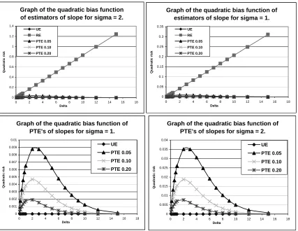
Figure 1: Graph of Quadratic Bias functions of the estimators for σ = 1, 2.
Obviously, the PTE is a biased estimator, and the amount of bias depends on the value ofG3,m(·),the non-centralF distribution function and the extent of departure of the
parameter from its value under null hypothesis. However, since 0 ≤G3,m(·) ≤1,the bias
of the PTE is always smaller than that of the RE, except for ∆ = 0. This is true for both ˆ
β and ˆθ.
quadratic bias function of the PTE is skewed to the right. At ∆ = 0 it starts for the origin and moves upward sharply until it reaches a pick for some moderate value of ∆ and then gradually declines to the horizontal axis. The quadratic bias of the PTE increases as the preselected level of significance decreases. This is quite clear from the lower pair of graphs in Figure 1. The quadratic bias function of the RE and PTE increases as the variance of the population becomes larger.
5
The risk of estimators
For any estimator, t∗ that estimates the parameter, µ,the quadratic error loss function is defined to be
L(t∗, W,µ) = (t∗−µ)0W(t∗−µ)
where W is a positive definite matrix of appropriate dimension. Then the risk of t∗ in estimatingµis the expected value ofL(t∗, W,µ).Thus for the slope and intercept vectors, the quadratic risk functions are given by
R(β∗, W2,β) = E(β∗−β)0W2(β∗−β) and R(θ∗, W1,θ) = E(θ∗−θ)0W1(θ∗−θ) (5.1)
whereβ∗andθ∗are the estimators ofβandθrespectively andW1andW2 are two positive definite matrices of appropriate dimensions. Therefore, the expressions of the quadratic risk for the UE of βand θ are obtained as
R1(˜β;W2) = E(˜β−β)0W2(˜β−β) =σ2tr(W2D2)
R1(˜θ;W1) = E(˜θ−θ)0W1(˜θ−θ) =σ2tr(W1D1) (5.2)
respectively. Similarly, the risks of the RE ofβ andθ are found to be
R2(ˆβ;W2) = E(ˆβ−β)0W2(ˆβ−β) =σ2 1
nQtr(W2J ∗) +
δ0W2δ
R2(ˆθ;W1) = E(ˆθ−θ)0W1(ˆθ−θ) =σ2tr(W1D11) +δ0T0W1T δ (5.3)
whereJ∗ =l
2l02.and D11= Λ +nQ1 tt0 in which Λ = Diag{n11,n12} and t0 = (¯x1,x¯2). Now, for the PTE, the quadratic risk expressions are given by
R3(ˆβpt;W2) = E(ˆβpt−β)0W2(ˆβpt−β) =σ2tr(W2D2)n1−G3,m(lα; ∆)
o
+δ0W2δ n
2G3,m(lα; ∆)−G5,m(l∗α; ∆)
o
R3(ˆθ
pt
;W1) = E(ˆθ
pt
−θ)0W 1(ˆθ
pt
−θ) =σ2tr(W1D11) n
1−G3,m(lα; ∆)
o
+δ0T0W1T δ n
2G3,m(lα; ∆)−G5,m(l∗α; ∆)
o
. (5.4)
5.1 Risk analysis for estimators of slope
The comparisons of the risks are useful in studying the relative performances of the estimators and thereby selecting an appropriate estimator in a given situation. In this subsection we provide both the analytical and graphical analyses of the quadratic risk function of the estimators of the shape parameter.
Comparison of UE and RE
First consider the difference of the risks of the UE and the RE,
N12(˜β,βˆ;W2) =R1(˜β;W2)−R2(ˆβ;W2) =σ2tr(W2D2)−
σ2
nQtr(W2J ∗)−
δ0W2δ. (5.5)
Thus the value ofN12(˜β,βˆ;W2) is positive zero or negative depending on
δ0W2δ
σ2
>
=
<tr
³
W2 h
D2−
J∗ nQ
i´
. (5.6)
Therefore, the performance of the estimators depends on the value of δ. The RE over performs the UE if the actual value of the slope parameter is not far from its value under
H0. Otherwise, ˜β dominates ˆβ. For further comparisons, note that by Courant Theorem (c.f. Puri and Sen, 1971, p.122) we have
λ1 ≤
h δ0W2δ
δ0D−1 2 δ
i
≤λ2 (5.7)
where λ1 is the smallest and λ2 is the largest characteristic roots of the matrix [W2D2].
Then we have ∆λ1≤hδ0W2δ
σ2
i
≤∆λ2.Thus the risk of RE is bounded in the following way
R1(˜β;W2) + ∆λ1− σ
2
nQtr(W2J ∗
)≤R2(ˆβ;W2)≤R1(˜β;W2) + ∆λ2− σ
2
nQtr(W2J ∗
). (5.8)
Clearly, when H0 is true then ∆ = 0 and the bounds are equal. In a special case, if
W2 =D−21 we get
tr(W2D2)
λ2 =
tr(W2D2)
λ1 = 2 and the difference between the risks becomes
N12(˜β,βˆ;W2) >=
< 0 according as ∆ <
=
> 2. (5.9)
In another special case, if W2 =I2 then RE is superior to the UE if ∆≤ tr(W2D2)
λ2 , which
depends on the value of the elements of the matrix D2.
Comparison of UE and PTE
The risk-difference of the UE and the PTE is given by
N13(˜β,βˆpt;W2) = R1(˜β;W2)−R3(ˆβpt;W2) =σ2tr(W2D2)G3,m(lα; ∆)
−δ0W2δ n
2G3,m(lα; ∆)−G5,m(l∗α; ∆)
o
Thus we have
N13(˜β,βˆ
pt
;W2) >=< 0 whenever
δ0W2δ
σ2
>
=
<
tr(W2D2)G3,m(lα; ∆)
n
2G3,m(lα; ∆)−G5,m(l∗α; ∆)
o. (5.11)
Then the bounds ofR3(ˆβ
pt
;W2) can be expressed as
RL3(ˆβpt;W2)≤R3(ˆβpt;W2)≤RU3(ˆβpt;W2) (5.12)
where
RL3(ˆβpt;W2) = R1(ˆβ
pt
;W2) + ∆λ1 n
2G3,m(lα; ∆)−G5,m(lα∗; ∆)
o
RU3(ˆβpt;W2) = R1(ˆβ
pt
;W2) + ∆λ2 n
2G3,m(lα; ∆)−G5,m(lα∗; ∆)
o
. (5.13)
The bounds become equal when ∆ = 0,that is, when H0 is true. But, under Ha
N13(˜β,βˆpt;W2) ≤ 0 if ∆≥ tr(W2D2)G3,m(lα; ∆) λ1
n
2G3,m(lα; ∆)−G5,m(l∗α; ∆)
o
N13(˜β,βˆ
pt
;W2) ≥ 0 if ∆≤
tr(W2D2)G3,m(lα; ∆)
λ2 n
2G3,m(lα; ∆)−G5,m(l∗α; ∆)
o. (5.14)
In a special case, if W2 =D−21 the difference between the risks becomes,
N13(˜β,βˆ
pt
;W2)>=<0 according as ∆ <=>
2G3,m(lα; ∆)
n
2G3,m(lα; ∆)−G5,m(lα∗; ∆)
o. (5.15)
Furthermore, under H0, ∆ = 0 and hence the risk of the PTE reduces to
R03(ˆβpt;W2) =σ2tr(W2D2)n1−G3,m(lα; 0)
o
(5.16)
which is less than that of the UE. But as ∆ moves away from 0, the risk of the PTE increases and reaches a maximum at ∆α (say) after crossing the line ∆0α given by (5.17)
then decreases towardsσ2tr(W2D2),the risk of the UE as ∆→ ∞. Comparison of PTE and RE
The difference between the quadratic risks of the PTE and the RE is
N32(ˆβ
pt
,βˆ;W2) = R3(ˆβ
pt
;W2)−R2(ˆβ;W2) =σ2tr(W2D2) n
1−G3,m(lα; ∆)
o
−δ0W2δ n
1−2G3,m(lα; ∆)−G5,m(l∗α; ∆)
o
. (5.17)
Thus we get
N32(ˆβpt,βˆ;W2)>=
<0 according as δ0W2δ
σ2
>
=
<
tr(W2D2) n
1−G3,m(lα; ∆)
o
n
1−2G3,m(lα; ∆)−G5,m(l∗α; ∆)
Graph of the quadratic risk function of estimators of slope for sigma = 1.
0 2 4 6 8 10 12 14 16 18
0 2 4 6 8 10 12 14 16 18
Delta Q u a d ra ti c ri s k UE RE PTE 0.05 PTE 0.10 PTE 0.20
Graph of the quadratic risk function of estimators of slope for sigma = 2.
0 10 20 30 40 50 60 70
0 2 4 6 8 10 12 14 16 18
Delta Q u a d ra ti c ri s k UE RE PTE 0.05 PTE 0.10 PTE 0.20
Graph of the quadratic risk function of PTE's of slope for sigma = 2.
0 2 4 6 8 10 12 14 16
0 2 4 6 8 10 12 14 16 18
Delta Q u a d ra ti c ri s k UE PTE 0.05 PTE 0.10 PTE 0.20
Graph of the quadratic risk function of PTE's of slope for sigma = 1.
0 0.5 1 1.5 2 2.5 3 3.5 4
0 2 4 6 8 10 12 14 16 18
[image:11.595.86.493.93.412.2]Delta Q u a d ra ti c ri s k UE PTE 0.05 PTE 0.10 PTE 0.20
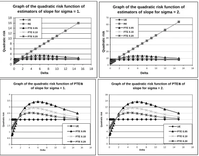
Figure 2: Graph of Quadratic Risk functions of the estimators for σ= 1, 2.
Therefore,
N32(ˆβ
pt
,βˆ;W2) ≥ 0 if ∆≤
tr(W2D2) n
1−G3,m(lα; ∆)
o
λ1 n
1−2G3,m(lα; ∆)−G5,m(lα∗; ∆)
o and
N32(ˆβ
pt
,βˆ;W2) ≤ 0 if ∆≥
tr(W2D2) n
1−G3,m(lα; ∆)
o
λ2 n
1−2G3,m(lα; ∆)−G5,m(lα∗; ∆)
o. (5.19)
Under H0, ∆ = 0 and hence the risk-difference reduces to σ2tr(W2D2) n
1−G3,m(lα; 0)
o
,
which is always positive. Thus the RE performs better than the PTE when H0 is true. In a special case, when W2 =D−21,
N32(ˆβpt,βˆ, W2)>=
<0 according as ∆ >
=
<
2n1−G3,m(lα; ∆)
o
n
1−2G3,m(lα; ∆)−G5,m(l∗α; ∆)
o. (5.20)
increase in the value of σ. The quadratic risk of the RE is unbounded and increases as the value of ∆ grows large. Nevertheless, it has smaller risk than the UE when the null hypothesis is true as well as when ∆ is very small. But for larger values of ∆, the RE performs the worst. The quadratic risk function of the PTE depends on the selected level of significance. It is an inverse function of α for all ∆. When the null hypothesis is true, the PTE has a smallest risk among the three estimators, regardless of the value ofα. This domination of the PTE continues up to some small value of ∆, (say ∆P), and than the
risk function of the PTE crosses that of the UE from the bottom and slowly grows up to maximum for some moderate value of ∆. Then it declines gradually towards the risk curve of the UE. The bottom two graphs show the behaviour of the PTE with the change of α
and σ.
From the analytical results and graphical representation it is evident that there is no clear cut domination of one single estimator over the others for all values of ∆. If it is known that the null hypothesis is true, the RE is the best choice. But in real life, this is hardly the case. So, for unknown ∆, the RE could be the worst. The PTE is better than the UE is ∆ is small or very large. For moderate values of ∆, the PTE is worse than the UE. This is more so when α is small.
5.2 Risk analysis for estimators of intercept
Finally, we compare the performances of the estimators of the intercept parameter vector based on the quadratic risk criterion.
Comparison of UE and RE
First consider the difference between the risks of the UE and the RE,
H12(˜θ,θˆ;W1) =R1(˜θ;W1)−R2(ˆθ;W1) =σ2tr(W1D1)−σ2tr(W1D11)−δ0T0W1T δ. (5.21)
Thus the value ofH12(˜θ,θˆ;W1) is negative, zero or positive depending on
∆T >=< tr(W1D11)−tr(W1D1) =tr(W1T0D2T)− ¯ x0W1¯x
nQ with ∆T =
δ0T0W1T δ
σ2 . (5.22)
Note that the matrix [W1T0D2T]−¯x 0W
1¯x
nQ is positive semi-definite. Therefore, sinceT is not
zerotr(W1[D1−D11])≥0.From (5.27) it is evident that whenδis close to zero RE performs better than the UE. On the other hand, as δ moves away from zero δ0TW1T δ → ∞, and hence the risk difference grows unboundedly. Then the UE performs better than the RE. Therefore, the UE is superior to the RE whenever
δ0T0W1T δ
σ2 > tr(W1T 0D
2T)− ¯ x0W1x¯
nQ . (5.23)
Comparison of UE and PTE
The risk-difference of the UE and the PTE is given by
H13(˜θ,θˆ
pt
;W1 ) = R1(˜θ;W1)−R3(ˆθ
pt
;W1) =σ2tr(W1[D1−D11])G3,m(lα; ∆)
−δ0T0W1T δ n
2G3,m(lα; ∆)−G5,m(l∗α; ∆)
o
. (5.24)
Thus we have
H13(˜θ,θˆ
pt
;W1)>=< 0 whenever
δ0T0W1T δ
σ2
<
=
>
tr(tr(W1[D1−D11])G3,m(lα; ∆)
n
2G3,m(lα; ∆)−G5,m(l∗α; ∆)
o . (5.25)
In a special case, whenW1= (D1−D11)−1 then (5.30) becomes
δ0T0[D1−D11]−1T δ
σ2
<
=
>
2G3,m(lα; ∆)
n
2G3,m(lα; ∆)−G5,m(lα∗; ∆)
o. (5.26)
Comparison of PTE and RE
The difference between the risks of the PTE and the RE is
H32(ˆθ
pt
,θˆ;W1) =R3(ˆθ
pt
;W1)−R2(ˆθ;W1) =σ2tr(W1[D1−D11) n
1−G3,m(lα; ∆)
o
−δ0T0W1T δn1−2G3,m(lα; ∆)−G5,m(l∗α; ∆)
o
. (5.27)
Now, from (5.32) we get H32(ˆθpt,θˆ;W1) <=
> 0 according as
δ0T0W1T δ
σ2
>
=
<
tr(W1[D1−D11]) n
1−G3,m(lα; ∆)
o
h
2n1−2G3,m(lα; ∆)
o
−n1−G5,m(lα∗; ∆)
oi (5.28)
where n1−2G3,m(lα; ∆)−G5,m(l∗α; ∆)
o
= h2n1−2G3,m(lα; ∆)
o
−n1−G5,m(lα∗; ∆)
oi
.
Therefore, based on (5.33), RE performs better than the PTE if
∆T <
tr(W1[D1−D11]) n
1−G3,m(lα; ∆)
o
λ2 h
2n1−2G3,m(lα; ∆)
o
−n1−G5,m(lα∗; ∆)
oi (5.29)
and the PTE dominates over the RE whenever
∆T >
tr(W1[D1−D11])n1−G3,m(lα; ∆)
o
λ1h2n1−2G3,m(lα; ∆)
o
−n1−G5,m(l∗α; ∆)
oi. (5.30)
h
Scatterplot of allergy rating for drug A & B
Indipendent Variable
14 12
10 8
6 4
2 0
Response Variable
20
18
16
14
12
10
8
6
4
2
0
Drug
Drug B
[image:14.595.96.463.93.391.2]Drug A
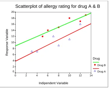
Figure 3: Graph of two fitted regression lines for the allergy data.
6
An example
To demonstrate the application of the method, we consider a data set from Weber and Skillings (2000, p.516). The study involves two drugs (A and B) for their effectiveness on testing allergies. Six people suffering from allergies were randomly allocated the the drugs, each one week apart. The severity of the allergy rated on a twenty-point scale before taking the drug, label asX, and after the drug, label asY. Regression lines ofY onX have been fitted to the data for the two drugs separately. The scatterplot and the fitted regression lines are given in Figure 3. The fitted regression lines for the two data sets are
ˆ
yA= 3.86 + 0.88xA, and ˆyB = 8.91 + 0.77xB. (6.1)
6.1 Determination of optimal level of significance
The outcome of the preliminary test depends on the level of significance, so is the preliminary test estimator. Therefore, search for an optimal level of significance is obvious. Here the optimality of the level of significance is in the sense of miniminsing the maximum risk of an estimator. One method to obtain an optimal level of significance is to use the Akaike’s (1972) Information Criterion or (AIC) as an abbreviation. Hirano (1977) used this approach to find the optimal level of significance. Khan and Saleh (1997) used the method in the linear regression model with Student-t errors.
For the model at hand we have 4 regression parameters and let the unrestricted parame-ter space be denoted by Ω. Under the null hypothesis, there are two regression parameparame-ters, and let the associated parameter space be denoted by Ω0. Let the likelihood function under the unrestricted parameter space be denoted by L(Ω) and that under the null hypothesis be L(Ω0). The corresponding AICΩ can be written as −2logeL( ˜Ω) + 2×4 and AICΩ0
can be written as −2logeL( ˆΩ0) + 2×2 respectively. Then following Hirano (1977), the
AIC criterion for the model, AICΩ˜ −AICΩˆ0 > 0 turns our to be −2logeλ < 4, where
λ= L( ˜Ω)
L( ˆΩ0),in which,L( ˜Ω) is the unrestricted maximum of the likelihood function andL( ˆΩ)
is the maximum of the likelihood function under the null hypothesis. Since, for the current model, asymptotically −2logeλ follows a χ22 distribution, the optimal level of significance based on the AIC criterion becomes P(χ22 <4) = 0.1353. This optimal value of the level of significance can be used in the process of the preliminary test decision.
7
Concluding remarks
parallel regression models.
Acknowledgements
The author thankfully acknowledges some valuable suggestions of two unknown referees as well as Dr. M.I. Bhatti, that helped improve an earlier version of the paper.
References
Akaike, H. (1972). Information theory and an extention of maximum likelihood principle. Problems of Control and Informationn Theory. Academiai Kiado, Hungarian Academy of Science, 202-212.
Ali, A.M. and Saleh, A.K.Md.E. (1990). Estimation of the mean vector of a multivariate normal distribution under symmetry. Jou. Statist. Comp. Simul.,35, 209-226. Bancroft, T.A. (1944). On biases in estimation due to the use of preliminary tests of
significance. Ann. Math. Statist.,15, 190-204.
Bancroft, T.A. (1964). Analysis and inference for incompletely specified models involving the use preliminary test(s) of significance. Biometrics,20, 427-442.
Bancroft, T.A. (1972). Some recent advances in inference procedures using preliminary tests of significance. In Statistical Papers in honour of G.W. Snedecor, Iowa State Univ. Press, 19-30.
Bhoj, D.S. and Ahsanullah, M. (1993). Estimation of conditional mean in a linear regression model. Biometrical Journal,35, 791-799.
Bhoj, D.S. and Ahsanullah, M. (1994). Estimation of a conditional mean in a regression model after a preliminary test on regression coeficient . Biometrical Journal, 36, 153-163.
Han, C.P. and Bancroft, T.A. (1968). On pooling means when variance is unknown. Jou. Amer. Statist. Assoc.,29, 21-34.
Hirano, K. (1977). Estimation with procedures based on preliminary test, shrinkage tech-nique and information criterion, Ann. Inst. Statist. Math., Vol. 1, 361-379.
Judge, G.G. and M.E. Bock (1978). The statistical implication of pre-test and Stein-rule estimators in econometrics. North-Holland, New York.
Khan, S. and A.K.Md.E. Saleh (1997). Shrinkage pre-test estimator of the intercept param-eter for a regression model with multivariate Student-t errors. Biometrical Journal, Vol. 29, 131-147.
Khan, S. and A.K.Md.E. Saleh (1995). Preliminary test estimators of the mean for sampling from some Student-t populations. Journal of Statistical Research, Vol. 29, 67-88. Kitagawa, T. (1963). Estimation after preliminary tests of significance. University of
California Publications in Statistics, 3, 147-186.
Mahdi, T.N., Ahmad, S.E. and Ahsanullah, M. (1998). Improved predicitons: Pooling two identical regression lines. Jou. Appld. Statist. Sc.,7, 63-86.
Puri, M.L. and Sen, P.K. (1973). Nonparametric Methods in Multivariate Analysis. Wiley, New York.
Saleh, A.K.Md.E. and Han, C.P. (1990). Shrinkage estimation in regression analysis. Es-tadistica, 42, 40-63.
Saleh, A.K.Md.E. and Sen, P.K. (1978). Non-parametric estimation of location parameter after a preliminary test on regression. Annals of Statistics,6, 154-168.
Sen, P.K and Saleh, A.K.Md.E. (1985). On some shrinkage estimators of multivariate location. Annals of Statistics. 13, 272-281.