Approximation of function and its derivatives using radial basis function networks

(1)

Approximation of Function and Its Derivatives

Using Radial Basis Function Networks

Nam Mai-Duy and Thanh Tran-Cong

Faculty of Engineering and Surveying,

University of Southern Queensland, Toowoomba, QLD 4350, Australia

Submitted to

Applied Mathematical Modelling

, December 2000 revised

August 2002

Abstract

. This paper presents a numerical approach, based on Radial Basis Function Networks (RBFNs), for the approximation of a function and its derivatives (scattered data interpolation). The approach proposed here is called the indirect radial basis function network (IRBFN) approximationwhich is compared with the usual directapproach. In the direct method (DRBFN) the closed form RBFN approximating function is rst obtained from a set of training points and the derivative functions are then calculated directly by dierentiating such closed form RBFN. In the indirect method (IRBFN) the formulation of the problem starts with the decomposition of the derivative of the function into RBFs.

Corresponding author: Telephone +61 7 46312539, Fax +61 7 46 312526, E-mailtrancong@usq.edu.au

(2)

The derivativeexpression is then integrated to yield an expression for the original function, which is then solved via the general linear least squares principle, given an appropriate set of discrete data points. The IRBFN method allows the ltering of noise arisen from the interpolation of the original function from a discrete set of data points and produces a greatly improved approximation of its derivatives. In both cases the input data consists of a set of unstructured discrete data points (function values), which eliminates the need for a discretisation of the domain into a number of nite elements (FE). The results obtained are compared with those obtained by the Feed Forward Neural Network (FFNN) approach where appropriate and the \Finite Element" methods. In all examples considered, the IRBFN approach yields a superior accuracy. For example, all partial derivatives up to second order of the function of three variables y = x2

1 +x

1x2

;2x

2 2

; x

2x3 +x

2

3 are

approximated with at least an order of magnitude better in the L2-norm in comparison

with the usual DRBFN approach.

Keywords: Radial basis function networks, function approximation, derivative

(3)

1 Introduction

(4)

(5)

2 Description of Problem

The problem considered in this paper is described as follows (superscripts are used to index elements of a set of neurons and subscripts denote scalar components of a p-dimensional vector):

Given a set of data points whose elements consist of paired values of the

indepen-dent variables (a vector x) and the dependent variable (a scalar y), denoted by fx

(i)y(i) gni

=1 wheren is the number of input points and

x= x

1x2:::xp]

T _where_p

is the number of dimensions and the superscript T _{denotes the transpose operation,}

nd a closed form approximate function f of the dependent variable y and its closed

form approximate derivative functions.

3 Function Approximation by RBFNs

An RBFN represents a map from the p-dimensional input space to the 1-dimensional output space f : Rp ! R

1 that consists of a set of weights

fw

(i) gmi

=1, and a set of radial

basis functions fg (i)

gmi

=1 where m

n. There is a large class of radial basis functions

which can be written in a general form g(i)(

x) =

(i)(

kx;c

(i)

k), where k:k denotes the

Euclidean norm and fc (i)

gmi

=1 is a set of the centers that can be chosen from among the

(6)

1. multiquadrics

(i)

(r) = (i)(

kx;c

(i)

k) =

p

r2+a(i)2 for somea

(i) > 0 (1)

2. inverse multiquadrics

(i)

(r) = (i)(

kx;c

(i)

k) =

1

p

r2+a(i)2 for some a

(i)> 0 (2)

3. Gaussians

(i)(r) = (i)(

kx;c

(i)

k) = exp

;

r2

a(i)2

for some a(i) > 0 (3)

wherea(i)is usually referred to as the width of theith basis function and r =

kx;c

(i)

k=

p

(x;c (i))

(x;c

(i)).

The inverse multiquadrics (2) and Gaussians function (3) have a local response, i.e. they decrease monotonically with increasing distance from the center (localized function). In contrast, the multiquadrics (1) increases with increasing distance from the center and therefore exhibits a global response (non-localized function). An important property of the RBFN is that it is a linearly weighted network in the sense that the output is a linear combination of m radial basis functions written as

f(x) =

m

X

i=1

w(i)g(i)(

(7)

With the model f constructed as a linear combination of m xed functions in a given family, the problem is to nd the unknown weightsfw

(i) gmi

=1. For this purpose, the general

least squares principle is used to minimise the sum squared error

SSE =Xn

i=1

y(i)

;f(x

(i))

2

(5)

with respect to the weights of f, resulting in a set of m simultaneous linear algebraic equations (normal equations) in the m unknown weights

(G

T

G)w =G

T

y (6)

where G= 2 6 6 6 6 6 6 6 6 6 6 4

g(1)( x

(1)) g(2)( x

(1))

g

(m)( x

(1))

g(1)( x

(2)) g(2)( x

(2))

g

(m)( x

(2))

... ... ... ... g(1)(

x

(n)) g(2)( x

(n))

g

(m)( x

(n)) 3 7 7 7 7 7 7 7 7 7 7 5

w = w

(1)w(2):::w(m)]T

y = y

(1)y(2):::y(n)]T.

However, in the special case where n = m, the resultant system is just

(8)

4 Function derivatives by direct RBFN method

In an arbitrary RBFN where the basis functions are xed and the weights are adaptable, the derivative of the function computed by the network is also a linear combination of xed functions (the derivatives of the radial basis functions). The partial derivatives of the approximate function f(x) (4) can be calculated as follows

@k_f

@xj:::@xl =fj:::l(x) =

m

X

i=1

w(i) @

k_g(i)

@xj:::@xl (8)

where @kg(i)

@xj:::@xl is the corresponding basis function for the derivative functionfj:::l(

x), which

is obtained by dierentiating the original basis function g(i)(

x) which is continuously

dierentiable. For example, considering the rst order derivative of function f(x) with

respect to xj, denoted by fj, the corresponding basis functions are found analytically as

follows:

1. for multiquadrics

h(i)(

x) = @g (i)

@xj = x j;c

(i)

j

(r2+a(i)2)0:5 (9)

2. for inverse multiquadrics

h(i)(

x) = @g (i)

@xj =;

xj;c (i)

j

(9)

3. for Gaussians

h(i)(

x) = @g (i)

@xj =

;2(xj ;c

(i)

j )

a(i)2 exp

;

r2

a(i)2

: (11)

Considering the second order derivative of function f(x) with respect to xj, denoted by

fjj, the corresponding basis functions will be

h(i)(

x) = @h (i)

@xj = r

2 +a(i)2

;(xj;c

(i)

j )2

(r2+a(i)2)1:5 (12)

2. for inverse multiquadrics h(i)(

x) = @h (i)

@xj = 3(x j ;c

(i)

j )2

(r2+a(i)2)2:5 ;

1

(r2+a(i)2)1:5 (13)

3. for Gaussians h(i)(

x) = @h (i)

@xj = 2a(i)2

2 a(i)2(xj

;c

(i)

j )2

;1 exp ; r2

a(i)2

: (14)

Similarly, the basis functions for fkj are as follows:

h(i)(

x) = @h (i)

@xk =;

(xj;c (i)

j )(xk ;c (i)

k )

(10)

2. for inverse multiquadrics h(i)(

x) = @h (i)

@xk = 3(x j;c

(i)

j )(xk;c (i)

k )

(r2+a(i)2)2:5 (16)

3. for Gaussians h(i)(

x) = @h (i)

@xk = 4(x j ;c

(i)

j )(xk ;c (i)

k )

a(i)4 exp

;

r2

a(i)2

: (17)

Once f(x) is determined by solving (6) or (7) for the unknown weights, which is referred

to as network training, it is straightforward and economical to compute its derivatives according to (8). However, this direct method has some drawbacks that are illustrated in the following example.

4.1 Example to illustrate the drawbacks of the DRBFN method

The function

y(x) = x3+

x + 0:5 ;3x2

is sampled at 50 uniformly spaced training points as depicted in Figure 1. Parameters to be decided before the start of network training are the number of centers m, their locations fc

(i) gmi

=1 and a set of the corresponding widths fa

(i) gmi

=1. The ideal data points

used here are not corrupted by noise. According to Cover's Theorem 9], the more basis functions are used, the better the approximation will be and so all data points will be taken to be the centers of the network (m = n) in this study. Thus fc

(i)= x

(i) gni

(11)

width of the ith basis function is determined according to the following relation 11]

a(i)=

d(i)

(18)

where is a factor, > 0, and d(i) is the distance from the ith center to the nearest

neighbouring center. As a measure of the accuracy of dierent approximate schemes, a norm of the error of the solution, Ne, is dened as

Ne =

v u u t

nt

X

i=1

(y(i)

;f

(i)) 2

(19)

where f(i) and y(i) are the calculated and exact function values at the point i, and nt is

the total number of test nodes. SmallerNes indicate more accurate approximations.

Table 1 shows the error norms Nes of the approximate function and its rst and

sec-ond derivatives that are obtained from the networks using dierent types of radial basis function based on a set of 250 test nodes. It can be seen that errors in the approximate function obtained from all networks are quite low and hence the global shape of the orig-inal function is well captured as shown in Figure 1. However, the derivative functions, especially higher order ones, are strongly inuenced by the local behaviour of the ap-proximant. The nature of a bad local behaviour despite a good global approximation is illustrated in Figure 2a. The errors in the function approximation amplify in the process of dierentiation as shown in Figures 2b-c with the corresponding error normsNes shown

(12)

However, the norms Nes of the derivative functions estimated using multiquadrics RBFs

are still quite high (Table 1). To improve accuracy, a new indirect method is proposed and presented in the next section.

5 Function derivatives by indirect RBFN method

It can be seen that the dierentiation process is very sensitive to even a small level of noise as illustrated in the previous section. In contrast it is expected that on average the integration process is much less sensitive to noise. Based on this observation, it is proposed here that the approximation procedure starts with the derivative function using RBFNs. The original function is then obtained by integration. Here the generic nature of \derivative function" and \original function" is illustrated as follows. Suppose a function f(x) and its derivatives f0(x) and f00(x) are to be approximated. The procedure consists

of two stages. In the rst stage, f(x) corresponds to the \original function" and f0(x) the

\derivative function". In the second stage the f0(x) obtained in stage 1 corresponds to

the \original function" andf00(x) the \derivative function". The procedure just discussed

(13)

5.1 Functions of one variable

5.1.1 IRBFN1 method

In this method, the rst order derivative function is decomposed into radial basis functions as

f0(x) =

m

X

i=1

w(i)g(i)(x) (20)

wherefg (i)(x)

gmi

=1is a set of radial basis functions and

fw

(i) gmi

=1 is the set of corresponding

weights. With this approximation, the original function can be calculated as

f(x) = Z f0 (x)dx = Z m X i=1

w(i)

g(i)

(x)dx = Xm

i=1

w(i) Z

g(i)

(x)dx =Xm

i=1

w(i)

H(i)

(x) + C1

(21) where C1 is the constant of integration and

fH

(i)(x) gmi

=1 is the set of corresponding basis

functions for the original function with H(i)(x) = R

g(i)(x)dx. The radial basis functions fg

(i) gmi

=1 are continuously integrable, but only two basis functions

fH

(i)(x) gmi

=1

(14)

H(i)

(x) = (x;c (i))

p

(x;c

(i))2+a(i)2

2 + a

(i)2

2 ln

(x;c (i)) +

q

(x;c

(i))2+a(i)2

(22) 2. for inverse multiquadrics

H(i)(x) = ln

(x;c (i)) +

q

(x;c

(i))2+a(i)2

: (23)

The training to determine the weights in (20) and (21) is equivalent to a minimisation of the following sum squared error

SSE =Xn

i=1

y(i)

;f(x

(i))

2

: (24)

Equation (21) is used in equation (24) in the minimisation procedure, which results in a system of equations in terms of the unknown weightsw(i). The data used in training the

network for the derivative and original functions just consists of a set of discrete values

fy (i)

gni

=1 of the dependent variable y and the closed form of the derivative function (20).

(15)

norm is the smallest in the least-squares sense, i.e. any combination of basis functions irrelevant to the t is driven down to a small value. After solving (24), a set of the weights is obtained and used for approximating the derivative function via (20) and together with the constant C1 for estimating the original function via (21). The example in section 4:1

is reconsidered here using the IRBFN1 method. The Nes over a set of 250 test nodes are

decreased considerably as shown in Tables 2 - 4. There is a signicant improvement in the results obtained by the IRBFN1 over those obtained by the DRBFN not only for the derivative functions but also for the original function. The improvement factor is dened as follows

Improvement factor = DRBFN N_IRBFN1_Ne_e: (25)

The improvementfactors are 102:6, 85:9 and 93:6 corresponding to the original, 1st deriva-tive and 2nd derivaderiva-tive functions respecderiva-tively when the multiquadricis used and 49:4, 40:6 and 44:7 when the inverse multiquadric is used (Tables 2-4).

5.1.2 IRBFN2 method

As an alternative indirect method for approximating function and its derivatives, the sec-ond order derivative functionf00(x) is rst approximated in terms of radial basis functions

as follows

f00(x) =

m

X

i=1

(16)

Then the rst derivative function f0(x) is given by (21) as

f0

(x) =

Z

f00

(x)dx =Xm

i=1

w(i)

H(i)

(x) + C1 (27)

with the basis functions given by (22) or (23). The original function is calculated as

f(x) =Z

f0(x)dx =

m

X

i=1

w(i)H(i)(x) + C

1x + C2 (28)

where C1 and C2 are constants of integration and the corresponding basis functions are

obtained by integrating (22) or (23) as shown below

H(i)(x) = Z

H(i)(x)dx = ((x

;c

(i))2+a(i)2)1:5

6 +

a(i)2

2 (x;c (i))ln

(x;c (i)) +

q

(x;c

(i))2+a(i)2

;

a(i)2

2

q

(x;c

(i))2+a(i)2 (29)

H(i)(x) = Z

H(i)(x)dx = (x

;c

(i))ln

(x;c (i)) +

q

(x;c

(i))2+a(i)2

; q

(x;c

(i))2+a(i)2: (30)

(17)

signicant for all approximate functions (more than 16 times). Thus, the multiquadric function maintains its superior performance in terms of accuracy among the radial basis functions used in IRBFN2.

5.1.3 The role of \constants" of integration

\Constants" of integration in equations (21) and (28) appear naturally in the present indirect formulation. The structure of the approximant therefore looks like

f(x) =Xm

i=1

w(i) H(i)(x) + polynomial: (31)

As a result, if y(x) is at or closer to a polynomial t, the above structure (31) has the ability for better accuracy. This is in addition to the inherent smoothing of error in the process of integration.

5.2 Functions of two or more variables

(18)

5.2.1 IRBFN1 method

Consider the approximation of a function of two variables f(x1x2). In the IRBFN1

method, the rst order partial derivative of f(x1x2) with respect to x1, denoted byf1,

is rst approximated in terms of radial basis functions

f1(x1x2) =

m

X

i=1

w(i)

g(i)

(x1x2) (32)

where fg (i)(x

1x2) gmi

=1 is a set of radial basis functions and

fw

(i) gmi

=1 is the set of

corre-sponding weights.

The original function can be calculated as

f(x1x2) = Z

f1(x1x2)dx1 =

Z m

X

i=1

w(i)g(i)(x

1x2)dx1

=Xm

i=1

w(i) Z

g(i)(x

1x2)dx1 =

m

X

i=1

w(i)H(i)(x

1x2) +C1(x2) (33)

whereC1(x2) is a function of the variablex2 and

fH

(i)(x 1x2)

gmi

=1 is the set of

correspond-ing basis functions for the original function and given below

H(i)(x

1x2) = (x 1

;c

(i)

1 )

p

r2 +a(i)2

2 + r2

;(x

1

;c

(i)

1 )

2+a(i)2

2 ln

(x1

;c

(i)

1 ) +

p

r2+a(i)2

(19)

H(i)

(x1x2) = ln

(x1

;c

(i)

1 ) +

p

r2+a(i)2

: (35)

The added term on the right hand side of (33) is a function of the variablex2 only. Thus

C1(x2) can be interpolated using the IRBFN2 method for univariate functions as follows

(in the previous section, IRBFN2 is shown to be the better alternative among the methods investigated in this work.)

C00 1(x

2) =

M

X

i=1

w(i)g(i)(x

2) (36)

C0 1(x

2) =

M

X

i=1

w(i)H(i)(x 2) +

b

C1 (37)

C1(x2) =

M

X

i=1

w(i)H(i)(x 2) +

b

C1x2+ b

C2 (38)

whereCb

1 and

b

C2are constants of integration w

(i) are the corresponding weights andM is

the number of centres whosex2 coordinates are distinct. Upon applying the general linear

least squares principle, a system of linear algebraic equations is obtained. The unknown of the system which is found by the SVD method as mentioned earlier, consists of the set of weights in (32), the second set of weights in (36) and the constants of integration

b

C1, b

C2. The strategy of approximation is the same for the derivative function off(x1x2)

(20)

5.2.2 IRBFN2 method

In this method, the second order derivative functions are rst approximated in terms of radial basis functions. For example, in the case of f11 the basis functions for the rst

derivative function, f1, are given by (34) or (35) while for the original function f, the

basis functions are obtained by integrating (34) or (35) and shown below

H(i)(x

1x2) =

Z

H(i)(x

1x2)dx1 = (r

2+a(i)2)1:5

6 +

r2

;(x

1

;c

(i)

1 )

2+a(i)2

2 (x1

;c

1)ln

(x1

;c

(i)

1 ) +

p

r2+a(i)2

;

r2

;(xj ;c

(i)

j )2+a(i)2

2

p

r2+a(i)2 (39)

H(i)(x

1x2) =

Z

H(i)(x

1x2)dx1 =

(x1 ;c 1)ln (x1 ;c

(i)

1 ) +

p

r2+a(i)2

; p

r2+a(i)2: (40)

The original function is calculated as

f(x1x2) =

m

X

i=1

w(i)H (i)

(x1x2) +C1(x2)x1+C2(x2) (41)

where C1(x2) andC2(x2) are constants of integration which are interpolated in the same

(21)

For the purpose of illustration, some numerical results are presented in the next section.

6 Numerical results

In this section, examples of approximation of functions of one, two and three variables are given. As mentioned, the multiquadric function appears to be the better one in terms of accuracy among the basis functions considered and will be used to solve the example problems. The factor that inuences the accuracy of the solution is just chosen to be 2:0 until now. In the following examples, for the purpose of investigation of its eect, will take values over a wide range with an increment of 0:2. From the numerical experiments discussed shortly, it appears that there is an upper limit for above which the system of equations (6) or (7) is ill-conditioned, which is also observed by Tarwater 14]. In the present work, the value of is considered to reach an upper limit when the condition of the system matrix is O(1017), i.e. the estimate for the reciprocal of the condition of the

matrix in 1-norm using LINPACK condition estimator 15] is of O(10;17).

6.1 Example 1

Consider the following function of one variable

y = 0:02(12 + 3x;3:5x

(22)

with 0 x 1, a problem studied by Hashem and Schmeiser 16]. They reported a

method, namely Mean Squared Error-Optimal Linear Combinations of Trained Feedfor-ward Neural Netwoks (MSE-OLC), for an approximation of the function and its deriva-tives. The authors suggest that the usual approach is to try a multiple of networks with possibly dierent structures and values for training parameters and the \best" net-work (based on some optimality criterion) is selected. Instead of the usual approach just described the authors investigated a new approach where a combination of the trained networks is constructed by forming the weighted sum of the corresponding outputs of the trained networks. The authors claim that their MSE-OLC method yields more accu-rate approximations in comparison with the best trained FFNN. For this problem, with a set of 200 training nodes and 10000 test nodes, the resultant MSEs for the original, the rst and second order derivative functions produced by MSE-OLC are 0:000017, 0:1 and 133:3, respectively, which are 87:3%, 69:7% and 64:5%, respectively, less than the MSEs produced by the best FFNN 16]. Here, both the direct and indirect RBFN meth-ods are applied to solve this problem using 200 training points and 10,000 test nodes, uniformly spaced along the x-axis. The training points are displayed in Figure 4a. In contrast, Hashem and Schmeiser 16] used the same number of data points but randomly distributed. In order to compare the present results with those obtained by Hashem and Schmeiser 16] the latter's MSEs are converted into norms Nes as dened in this paper.

Thus the norms Nes corresponding to the original, rst derivative and second derivative

(23)

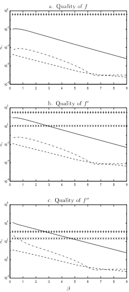
of approximation improves signicantly with RBFN, and particularly that the IRBFN1 yields superior results over the whole range of values of (e.g. with = 9 the Nes

for the second derivative are 0:0877 (IRBFN1), 5:6869 (DRBFN), 209:89 (conventional) and 1154:56 (MSE-OLC) 16]). Even more accurate results can be obtained by using the second indirect method IRBFN2 (Ne= 0:0517), as shown in the same Figure 3. Figure 4

shows the plots of the function and its derivative at = 0:2 obtained with the IRBFN2 where the \worst" value of is used to demonstrate the superior performance of the IRBFN2.

6.2 Example 2

Consider the following bivariate function

y = x2 1x

2+x

3 2=3 + x

2

2=2

where ;3 x 1

3 and ;3 x 2

3. This is a non-trivial example which has a

complicated root structure 17]. The data consist of 441 points, uniformly spaced along both axes x1 and x2 for training and 1764 points for testing. The results obtained from

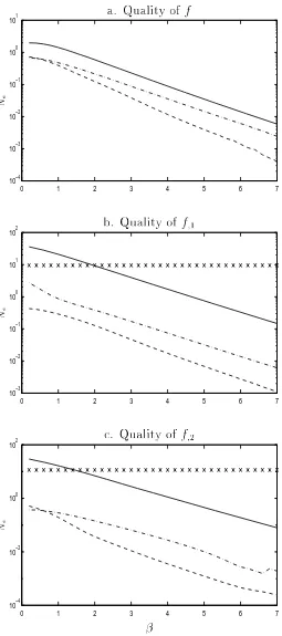
both DRBFN and IRBFN methods are compared with the accuracies achieved by the conventional method using linear shape function over triangular elements. Figure 5 shows the quality of the approximation of the function f(x1x2) and its rst derivatives while

(24)

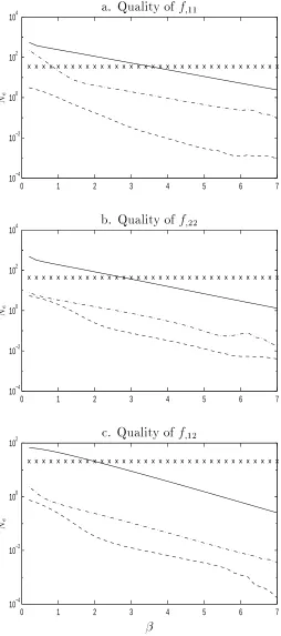
are more accurate with IRBFN2 as shown in Figures 5-6. Thus it can be seen that the IRBFN2 yields better performance than the IRBFN1 which in turn performs better than the DRBFN.

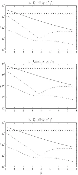
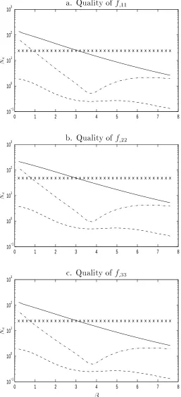
6.3 Example 3

Consider the following function of three variables

y = x2

1+x

1x2

;2x

2 2

;x

2x3+x 2 3

where 0 x 1

0:5, 0 x 2

0:5 and 0 x 3

0:5. In this example, 216 points,

uniformly spaced along the axes x1, x2 and x3, are used for training and 1728 points for

testing. Figure 7 shows the quality of the approximation of the original function. Figure 8 shows the plots of norm Ne as function of (0:2 7:6) for rst order derivative

functionsf1,f2 and f3, while Figures 9-10 are for second order derivative functionsf11,

f22, f33, f12, f23 and f31. Figures 7-10 again show that the IRBFN2 method exhibits

superior performance over other methods.

7 Concluding Remarks

(25)

indi-rect RBFN method are able to oer better results in comparison with the conventional method using linear shape functions. The present RBFN methods also eliminate the need for FE-type discretisation of the domain of analysis. Among the RBFs considered, multiquadrics RBF oers the best performance in accuracy in both DRBFN and IRBFN method. Numerical results show that IRBFNs, especially IRBFN2, achieve greater accu-racy than DRBFN in the approximation of both function and especially its derivatives. Furthermore, this superior accuracy is maintained over a wide range of RBF's width (0:2 < < 9). A formal theoretical proof of the superior accuracy of the present IRBFN method cannot be oered at this stage, at least by the present authors. However, a heuristic argument can be presented as follows. In the direct methods, the starting point is the decomposition of the unknown functions into some nite basis and all derivatives are obtained as a consequence. Any inaccuracy in the assumed decomposition is usually magnied in the process of dierentiation. In contrast, in the indirect approach the start-ing point is the decomposition of the highest derivatives into some nite basis. Lower derivatives and nally the function itself are obtained by integration which has the prop-erty of damping out or at least containing any inherent inaccuracy in the assumed shape of the derivatives. At this stage, it is recommended that the IRBFN2 method is the better one among the methods considered for an accurate approximation of a function and its derivative. In a subsequent study, the application of the DRBFN and IRBFN methods in solving dierential equations will be reported.

Acknowledgements

(26)

(27)

References

1

] R.D. Cook, D.S. Malkus, M.E. Plesha, Concepts and Applications of Finite Element Analysis, John Wiley & Sons, Toronto, 1989.

2

] C.A. Brebbia, J.C.F. Telles, L.C. Wrobel, Boundary Element Techniques: Theory and Applications in Engineering, Springer-Verlag, Berlin, 1984.

3

] M.J.D. Powell, Radial basis functions for multivariable interpolation: a review, in: J.C. Watson, M.G. Cox (Eds), IMA Conference on Algorithms for the Approxima-tion of FuncApproxima-tion and Data, Royal Military College of Science, Shrivenham, England, 1985, pp. 143-167.

4

] D.S. Broomhead, D. Lowe, Multivariable functional interpolation and adative net-works, Complex Systems 2 (1988) 321-355.

5

] M.J.D. Powell, Radial basis function approximations to polynomial, in: D.F. Griths, G.A. Watson (Eds), Numerical Analysis 1987 Proceedings, University of Dundee, Dundee, UK, 1988, pp. 223-241.

6

] T. Poggio, F. Girosi, Networks for approximation and learning, in: Proceedings of the IEEE 78, 1990, pp.1481-1497.

7

] F. Girosi, T. Poggio, Networks and the best approximation property, Biological Cy-bernetics 63 (1990) 169-176.

(28)

9

] S. Haykin, Neural Networks: A Comprehensive Foundation, Prentice-Hall, New Jer-sey, 1999.

10

] J. Park, I.W. Sandberg, Approximation and radial basis function networks, Neural Computation 5 (1993) 305-316.

11

] J. Moody, C.J. Darken, Fast learning in networks of locally-tuned processing units, Neural Computation 1 (1989) 281-294.

12

] R. Franke, Scattered data interpolation: tests of some methods, Mathematics of Computation 38(157) (1982) 181-200.

13

] W.H. Press, B.P. Flannery, S.A. Teukolsky, W.T. Vetterling, Numerical Recipes in C: The Art of Scientic Computing, Cambridge University Press, Cambridge, 1988.

14

] A.E. Tarwater, A parameter study of Hardy's multiquadrics method for scattered data interpolation, Technical Report UCRL-563670, Lawrence Livemore National Laboratory, 1985.

15

] J.J. Dongarra, J.R. Bunch, C.B. Moler, G.W. Stewart, LINPACK User's Guide, SIAM, Philadelphia, 1979.

16

] S. Hashem, B. Schmeiser, Approximating a function and its derivatives using MSE-optimal linear combinations of trained feedforward neural networks, in: Proceedings of the 1993 World Congress on Neural Networks, vol 1, Lawrence Erlbaum Asso-ciates, Hillsdale, New Jersey, 1993, pp. 617-620.

(29)

Table 1: Ne of the approximate function and its derivatives for = 2:0 with the

di-rect RBFN (DRBFN) approach. The quality of approximation deteriorates with higher derivatives.

Gaussians multiquadrics Inverse multiquadrics Original function 7:002e;01 9:570e;02 7:459e;01

(30)

Table 2: Comparison of Nes between the DRBFN and IRBFN1 for the original function,

= 2:0.

multiquadrics Inverse multiquadrics DRBFN 9:570e;02 7:459e;01

IRBFN1 9:324e;04 1:510e;02

(31)

Table 3: Comparison of Nes between the DRBFN and IRBFN1 for the 1st derivative

function, = 2:0.

multiquadrics Inverse multiquadrics DRBFN 4:053e + 00 3:086e + 01 IRBFN1 4:720e;02 7:603e;01

(32)

Table 4: Comparison of Nes between the DRBFN and IRBFN1 for the 2nd derivative

function, = 2:0.

(33)

Table 5: Comparison of Nes between the two indirect methods using multiquadrics for

= 2:0. Here the improvement factor is dened as the improvement of IRBFN2 relative to IRBFN1.

Original 1st derivative 2nd derivative IRBFN1 9:324e;04 4:720e;02 1:671e + 00

IRBFN2 3:968e;05 2:100e;03 1:022e;01

(34)

Table 6: Comparison ofNes between the two indirect methods using inverse multiquadrics

for = 2:0. Here the improvement factor is dened as the improvement of IRBFN2 relative to IRBFN1.

Original 1st derivative 2nd derivative IRBFN1 1:510e;02 7:603e;01 2:550e + 01

IRBFN2 2:200e;03 9:760e;02 4:073e + 00

(35)

−3 −2.5 −2 −1.5 −1 −0.5 0 0.5 1 1.5 2 −30

−25 −20 −15 −10 −5 0 5 10 15

training point exact approximate

x

y

f

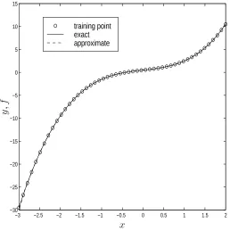
Figure 1: Function y(x) = x3+x + 0:5: plot of training points, the exact function and

[image:35.612.173.431.91.350.2]

(36)

1.75 1.8 1.85 1.9 1.95 2 7.5

8 8.5 9 9.5 10 10.5 11

1.75 1.8 1.85 1.9 1.95 2

0 5 10 15 20

1.75 1.8 1.85 1.9 1.95 2

−400 −300 −200 −100 0 100 200

x

y

f

y

0 f

0

y

0

0 f

00

a. Original function

b. First derivative

c. Second derivative

Figure 2: Function y(x) = x3+x + 0:5: Zoom in on the original, rst derivative and

sec-ond derivative functions ( = 2:0). Solid line: exact function and dashed line: DRBFN approximation using inverse multiquadrics. The plots illustrate the shortcomings of the DRBFN approach where the associated error norms are 7:459e;1, 3:086e+1 and 1:141e+3

[image:36.612.173.430.34.603.2]

(37)

0 1 2 3 4 5 6 7 8 9

10−8

10−6

10−4

10−2

100

0 1 2 3 4 5 6 7 8 9

10−6

10−4

10−2

100

102

0 1 2 3 4 5 6 7 8 9

10−2

100

102

104

106

Ne

a. Quality of f

b. Quality off0

c. Quality of f00

Figure 3: Approximantf of the function y = 0:02(12+3x;3:5x

2+7:2x3)(1+cos4x)(1+

0:8sin3x) and its derivatives: plots of the norm Neas a function of. Legends +:

[image:37.612.176.431.30.608.2]

(38)

0 0.1 0.2 0.3 0.4 0.5 0.6 0.7 0.8 0.9 1 0

0.2 0.4 0.6 0.8 1

0 0.1 0.2 0.3 0.4 0.5 0.6 0.7 0.8 0.9 1

−6 −4 −2 0 2 4 6 8

0 0.1 0.2 0.3 0.4 0.5 0.6 0.7 0.8 0.9 1

−150 −100 −50 0 50 100

x

y

f

y

0 f

0

y

0

0 f

00

a. Original function

b. First derivative

c. Second derivative

Figure 4: Function y = 0:02(12 +3x;3:5x

2+7:2x3)(1+cos4x)(1+0:8sin3x) and its

[image:38.612.174.432.33.603.2]

(39)

0 1 2 3 4 5 6 7

10−4

10−3

10−2

10−1

100

101

0 1 2 3 4 5 6 7

10−3

10−2

10−1

100

101

102

0 1 2 3 4 5 6 7

10−4

10−2

100

102

Ne

a. Quality of f

b. Quality of f1

c. Quality of f2

Figure 5: Approximantf of the function y(x1x2) =x 2 1x

2+x

3

2=3+x

2

2=2 and its derivatives:

plots of the norm Ne as a function of . Legends x: conventional element method, solid

[image:39.612.176.431.32.607.2]

(40)

0 1 2 3 4 5 6 7

10−4

10−2

100

102

104

0 1 2 3 4 5 6 7

10−4

10−2

100

102

104

0 1 2 3 4 5 6 7

10−4

10−2

100

102

Ne

a. Quality off11

b. Quality of f22

c. Quality of f12

Figure 6: Approximant of the derivatives of the function y(x1x2) =x 2 1x

2+x

3 2=3 + x

2 2=2:

[image:40.612.176.430.35.608.2]

(41)

0 1 2 3 4 5 6 7 8 10−4

10−3 10−2 10−1 100

Ne

a. Quality of f

Figure 7: Approximant of the function y = x2

1 +x

1x2

;2x

2 2

;x

2x3 +x 2

3: plots of the

norm Ne as a function of. Solid line: DRBFN, dashdot line: IRBFN1 and dashed line:

[image:41.612.177.431.186.451.2]

(42)

0 1 2 3 4 5 6 7 8

10−3

10−2

10−1

100

101

0 1 2 3 4 5 6 7 8

10−3

10−2

10−1

100

101

0 1 2 3 4 5 6 7 8

10−3

10−2

10−1

100

101

Ne

a. Quality of f1

b. Quality of f2

c. Quality of f3

Figure 8: Approximant of the derivatives of the function y = x2

1+x

1x2

;2x

2 2

;x

2x3+x 2 3:

[image:42.612.177.433.32.606.2]

(43)

0 1 2 3 4 5 6 7 8

10−1

100

101

102

103

0 1 2 3 4 5 6 7 8

10−1

100

101

102

103

0 1 2 3 4 5 6 7 8

10−1

100

101

102

103

Ne

a. Quality of f11

b. Quality of f22

c. Quality of f33

1+x

1x2

;2x

2 2

;x

2x3+x 2 3:

[image:43.612.175.432.37.601.2]

(44)

0 1 2 3 4 5 6 7 8

10−1

100

101

102

103

0 1 2 3 4 5 6 7 8

10−1

100

101

102

103

0 1 2 3 4 5 6 7 8

10−1

100

101

102

103

Ne

a. Quality of f12

b. Quality of f23

c. Quality of f31

Figure 10: Approximant of the derivatives of the functiony = x2

1+x

1x2

;2x

2 2

;x

2x3+x 2 3:

plots of the norm Ne as a function of. Solid line: DRBFN, dashdot line: IRBFN1 and

[image:44.612.176.432.36.613.2]

(45)

Abbreviated title for running headline

(46)

Figure Captions

Figure 1: Function y(x) = x3+x + 0:5: plot of training points, the exact function and

the approximate function obtained by the direct RBFN using inverse multiquadrics basis functions (DRBFN) with = 2:0: Note that the accuracy of the approximation of the function is such that the error (i.e. the dierence between the dashed and the solid lines) is not discernible on this plot. However, the goodness of the global shape might not be good enough in obtaining accurate function derivatives as illustrated in the next Figure 2.

Figure 2: Function y(x) = x3+x + 0:5: Zoom in on the original, rst derivative and

sec-ond derivative functions ( = 2:0). Solid line: exact function and dashed line: DRBFN approximation using inverse multiquadrics. The plots illustrate the shortcomings of the DRBFN approach where the associated error norms are 7:459e;1, 3:086e+1 and 1:141e+3

for the approximation of the function, its rst derivative and second derivative respec-tively.

Figure 3: Approximantf of the function y = 0:02(12+3x;3:5x

2+7:2x3)(1+cos4x)(1+

0:8sin3x) and its derivatives: plots of the norm Neas a function of. Legends +:

MSE-OLC, x: conventional element method, solid line: DRBFN, dashdot line: IRBFN1 and dashed line: IRBFN2.

Figure 4: Function y = 0:02(12 +3x;3:5x

2+7:2x3)(1+cos4x)(1+0:8sin3x) and its

(47)

that the numerical approximation and the analytical plots are not discernible. The data points are also shown as .

Figure 5: Approximantf of the function y(x1x2) =x 2 1x 2+x 3 2=3+x 2

2=2 and its derivatives:

line: DRBFN, dashdot line: IRBFN1 and dashed line: IRBFN2. It can be seen that the quality of the approximation for the derivatives is much better with the IRBFN approach. Figure 6: Approximant of the derivatives of the function y(x1x2) =x

2 1x

2+x

3 2=3 + x

2 2=2:

line: DRBFN, dashdot line: IRBFN1 and dashed line: IRBFN2. It can be seen that the quality of the approximation for the derivatives is much better with the IRBFN approach. Figure 7: Approximant of the function y = x2

1 +x

1x2

;2x

2 2

;x

2x3 +x 2

3: plots of the

norm Ne as a function of. Solid line: DRBFN, dashdot line: IRBFN1 and dashed line:

IRBFN2. It can be seen that the quality of the approximation is much better with the IRBFN approach.

1+x

1x2

;2x

2 2

;x

2x3+x 2 3:

line: DRBFN, dashdot line: IRBFN1 and dashed line: IRBFN2. It can be seen that the quality of the approximation is much better with the IRBFN approach.

1+x

1x2

;2x

2 2

;x

2x3+x 2 3:

(48)

quality of the approximation is much better with the IRBFN approach. Figure 10: Approximant of the derivatives of the functiony = x2

1+x

1x2

;2x

2 2