Faraday waves in radial outflow

(1)

TALL EUCALYPT FORESTS OF

AUSTRALIA: STRUCTURE,

PATTERN AND PROCESS

Jessie C. Buettel

B.Sc. (Hons) UTas

School of Biological Sciences – University of Tasmania

TAS 7001 AUSTRALIA

Thesis submitted in fulfilment of the requirements for the

Degree of

Doctor of Philosophy

(2)

(3)

DECLARATION

This thesis contains no material which has been accepted for the award of any other degree or diploma in any tertiary institution, and to the best of my knowledge and belief, contains no material previously published or written by another person, except where due reference is made in the text of the thesis, nor does the thesis contain any material that infringes copyright. The publishers of the papers comprising all chapters, hold the copyright for that content, and access to the material should be sought from the respective journal. The remaining non-published content of the thesis may be made available for loan and limited copying and communication in accordance with the Copyright Act 1968.

Date Signed

18 June 2017

(4)

STATEMENT OF ETHICAL CONDUCT

The research associated with this thesis abides by the international and Australian codes on human and animal experimentation, the guidelines by the Australian Government's Office of the Gene Technology Regulator and the rulings of the Safety, Ethics and Institutional Biosafety Committees of the University.

Date Signed

18 June 2017

(5)

STATEMENT OF PUBLISHED WORK

Candidate was the primary author on all chapters, undertook substantial fieldwork, and did most data analyses. For each respective chapter, the candidate as well as all co-authors contributed to developing the ideas. Barry W. Brook and Nicole Bezemer assisted with the field work – collecting fallen wood and topographic data that contributed to Chapters III, VI, VIII and IX. David M. J. S. Bowman provided access to the primary data used in Chapters III, IV, VI, VII and IX. Barry W. Brook, Stefania Ondei, George P. W. Perry, John Alroy, Andrew Cole and John Dickey contributed to some data analysis. The candidate as well as Barry W. Brook assisted with refining the text.

Supplementary Information for all chapters, including data and additional analyses, can be found here: https://ecological-dynamics.org/data/

The following papers have resulted from this Ph.D. thesis research:

Buettel, J.C., Bowman, D.M.J.S., Perry, G.L.W., Hovenden, M.J. & Brook, B.W. (2016) A global synthesis of reported spatial patterns in forests. Ecography (in review).

(6)

Buettel, J.C., Alroy, J. & Brook, B.W. (2017) Latitudinal controls on forest species richness are not direct. Nature Ecology and Evolution (in review).

Buettel, J.C., Ondei, S. & Brook, B.W. (2017) Look down to see what’s up: A systematic overview of treefall dynamics in forests. Forests 8, 123. doi:10.3390/f8040123.

Buettel, J.C., Ondei, S., Dickey, J.M., Cole, A.A. & Brook, B.W. (2017) Reading the forest logbook: environmental drivers of living and dead elements of Australian eucalypt forests. Diversity and Distributions (in review).

Buettel, J.C., Ondei, S. & Brook, B.W. (2017) Missing the wood for the trees? New ideas on defining forests and forest degradation. Rethinking Ecology (in press). doi: 10.3897/[email protected]

Buettel, J.C., Ondei, S. & Brook, B.W. (2017) A practical method for creating a digital topographic surface for ecological plots using ground-based measurements. Landscape Ecology (in review).

Buettel, J.C., Cole, A., Dickey, J.M. & Brook, B.W. (2017) Modelling linear spatial features in ecology. Ecology (in review).

Buettel, J. C., Brook, B.W., Cole, A.A., Dickey, J.M. & Flies, E.J. (2017) Interdisciplinary to transdisciplinary: shifting the collaboration paradigm for greater advances in science. Ecology and Evolution. (in review).

(7)

Additional publications candidate co-authored during PhD:

Brook, B.W. & Buettel, J.C. (2016) Emigration is costly but immigration has benefits in human-altered landscapes. Functional Ecology 30, 1478-1479. doi: 10.1111/1365-2435.12639.

Brook, B.W., Ellis, E.C. & Buettel, J.C. (2017) What is the evidence for planetary tipping points? Chapter 8 in: Effective Conservation Science: Data Not Dogma

(eds. P. Kareiva, M. Marvier & B. Silliman), Oxford University Press (in press). ISBN: 9780198808985.

Johnson, C. N., Balmford, A., Brook, B.W., Buettel, J.C., Galetti, M., Guangchun, L. & Wilmshurst, J.M. (2017) Biodiversity losses and conservation responses in the Anthropocene. Science 356, 270-275 (major review). doi: 10.1126/science.aam9317.

Signed: Signed:

Barry W. Brook Anthony Koutoulis

Supervisor Head of School

School of Biological Sciences School of Biological Sciences University of Tasmania University of Tasmania

(8)

ACKNOWLEDGEMENTS

There are many people that have been part of my journey these last 3.5 years, and the stress of forgetting anyone is almost equivalent to ‘waiting for the in-review status to change to awaiting editor decision for a manuscript submission!’ So, I will start by offering a sincere thank you to everyone that has had an impact on my PhD at any stage throughout my journey – you may not have been mentioned in these acknowledgments but be rest assured that my bad memory is the reason!

I would, first and foremost like to give a wholehearted thank you to my supervisor Barry Brook, for taking me under his wing and providing me with ample opportunities to grow and excel. There was never a challenge he thought I couldn’t rise to; his constant belief in my ability, and support and encouragement that he provided will remain with me for the rest of my career. I am proud, and sincerely blessed to have been under his tutelage.

My PhD would not have been possible without the AusPlots data and David Bowman’s belief that I would be able to do it justice. TERN (AusPlots), Sam Wood, Karl Rann and everyone associated with the funding and collection of these data – I am deeply grateful.

A massive thank you to Nicole Bezemer for her dedication and help with field work. We created some great memories on those trips.

(9)

Jon, I am deeply grateful for your friendship, guidance and support throughout this journey, I could not have done it without you.

I also wish to thank my close friends and family for their support and patience throughout this journey. My family’s mantra: ‘you are Jessie Buettel and you can do anything,’ is a perfect testament to their unwavering belief in me.

Stefania Ondei, you are amazing. That is all.

To the D.E.E.P lab – I appreciate your patience and encouragement during my PhD completion. You are a wonderful and fun group of people.

Sam Adlard, Ian Cover, Emily Flies, thank you for being there for me and believing in me – particularly through all the tough times.

A warm thanks to Scott Carver, Vector, Relly, (the puppas) and Lynx for being my rock(s) through turbulent times, and having such a positive influence on my life. Scott, I also would not have gotten through my Ph.D. without a coffee machine – best gift EVER!

I would also like to acknowledge the support of the Australian Postgraduate Award scholarship and the Multidisciplinary Environment Research Group (MERG) for providing financial support for myself and my innovative research endeavours.

(10)

SUMMARY

(11)

(12)

CHAPTER I

INTRODUCTION TO PATTERN

AND PROCESS IN FOREST

ECOLOGY

Forests are complex three-dimensional ecosystems whose structure and function are

shaped by biotic (living: plants, animals, micro-organisms) and abiotic (non-living:

environmental, physical) components. An overarching aim of forest ecology is to

isolate and understand each component, so as to build a picture of how they are

interrelated, and how they shape overall ecosystem function in synergy. In this

introductory chapter, I overview the main processes that influence forest structure,

describe how forest patterns develop and are maintained through time, and briefly

explore the methods currently used in forest-ecology research. I also introduce the

principal dataset used in this study (AusPlots), and describe the aims and key

(18)

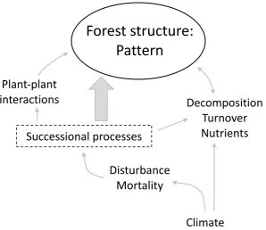
orests are the dominant land-based ecosystem worldwide by area, sequester almost half of the planet’s terrestrial surface carbon, and regulate climate at local to global scales (Pan et al. 2013a). Projected pressures due to global change, including expansion of agriculture and biofuels, forestry, and climate-driven shifts, pose significant threats to global forest biodiversity, structure and function (Meyfroidt

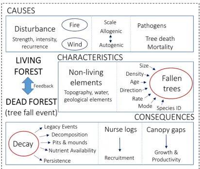
et al. 2010). Understanding how these pressures and threats might manifest over time is critical, particularly in the context of the conservation of these natural ecosystems. Ultimately, ecological processes such as succession, climate, plant-plant interactions, disturbance (fire, windthrow), decomposition, turnover, and nutrient availability and dynamics, are essential to the development of forest pattern (Fig. 1; Buettel et al.

2017). This spatial patterning and structure is further characterised by horizontal (niche differentiation, resource and water availability), and vertical (tree height, canopy, light availability) elements of variation, and it is the differences in these factors that give rise to complex forest structures (Franklin et al. 2002b). Pinpointing the underlying mechanisms that drive forest structure and tree distribution—that is, linking observed patterns to underlying processes—is key to predicting how forest dynamics will respond to disturbance and global change, given underlying differences in climate, species composition and distribution.

(19)

Development of forest pattern

Successional processes/forest age

Stand structure and forest composition is often conceptualised as a sequence of temporal snap-shots of ongoing primary or secondary successional processes (Box 1; Chen et al. 2004). In reality, successional processes create a continually shifting composition of species within the community, fluctuating as disturbances of different intensities, sizes and frequencies alter the landscape. The serial progression of tree species depicted in Box 1 is not random; certain species have evolved life histories to exploit the conditions that define each successional stage. As environmental

Forest structure:

Pattern

Plant-plant

interactions

Successional processes

Disturbance

Mortality

Climate

Decomposition

Turnover

Nutrients

[image:19.595.174.473.81.339.2]

(20)

conditions and disturbance frequencies change, a partially predictable sequence of habitats is created in which only a narrow suite of species can thrive (West et al. 2012). Once established, the residing species can alter key processes such as light intensity on the forest floor, soil composition, and the availability of nutrients in the environment, to ensure successional process (tree replacement) continues. In some environments, succession reaches a climax, which is characterised by a small number of dominant species that form a stable community, whilst in others, disturbance is a persistent feature that continually creates a flux of species diversity. Throughout this research thesis, I focus largely on communities that are in ‘dynamic equilibrium’ (i.e., consist of a diverse mix of species, including numerous mature trees, but experience continual small- to large-scale disturbances), and are dominated by a single genus,

(21)

Forest age, or time since last disturbance, is an important attribute of forest structure and succession as it influences size and density of the component species and the availability of resources like nutrients and light. Consequently, many deterministic processes during stand structural development, such as net primary production (NPP), mortality, biomass, and woody debris accumulation, are related to stand age (Spies 1998). Early successional forests have a higher proportion of fast-growing species and higher mortality rates due to intense competition for light and space among rapidly growing trees (Enquist and Niklas 2002). Therefore, these forests can achieve high woody productivity but relatively low wood density and biomass. In contrast, forests in later successional, or “old-growth” stages, are typified by a shade-tolerant

Box 1: Primary and secondary succession

Primary succession occurs from a baseline environment devoid of visible life. Environments are typified by soil or rock that has been impacted by, for example, lava flows, newly formed sand dunes or rock remaining from a retreating glacier.

Secondary succession occurs from a baseline of pre-existing life and nutrients that have been temporarily removed, either through small- to large-scale disturbances that retain environment functionality.

Box 1 figures: Two types of successional processes a) primary succession and b)

secondary succession. Source:

(22)

understory with a canopy of larger species that may have had relatively fast growth rates before reaching crown maturity, and decreased biomass growth after canopy closure (Ryan et al. 2004). By maintaining slow growth and low mortality on relatively nutrient-poor soils, these trees may survive for centuries and achieve a high biomass (Pan et al. 2013b). Consequently, each tree species within a forest is likely to exhibit a range of spatial patterns depending on the successional stage. Determining the frequency, intensity and duration of the processes that generate these patterns is essential for understanding how forest patterns develop over time..

Climate

(23)

distributions to occupy suitable climates, new forest communities assemble (Bertrand

et al. 2011; Zhu et al. 2012; Coomes et al. 2014). Therefore, climate is considered a strong predictor of current and future plant distributions, growth and forest structure.

Decomposition, turnover and nutrients

The availability of nutrients within an ecosystem depends on the input and efficient cycling of nutrients within and across communities (Prescott 2002). There are multiple pathways through which this is achieved: plant to soil, soil to plant (root uptake) and internal redistribution of nutrients (Sharma and Sharma 2004). Plants return nutrients to the soil as litter, comprising a mixture of fine (leaf litter, bark, twigs) and course material (branches and fallen trees), which are decomposed (Sharma and Sharma 2004). Decomposition and turnover are critical determinants of the global carbon cycle and nutrient turnover (Del Grosso et al. 2005; Parton et al. 2007), and are therefore paramount in shaping forest structure and pattern.

(24)

surrounding environment, such as chemical properties (determined in part by species identity), size, mode of death, microclimate, biotic community are collectively important for determining rates of turnover, decomposition and nutrient release in forests (Buettel et al. 2017). Understanding the properties and the spatial distribution of fallen wood may indeed be key to unlocking further information about forest structure and process.

Disturbance and mortality

The presence of fallen wood, fire scars on trees and position of standing dead trees are important indicators of disturbance and/or mortality. Such events are often unpredictable, random (i.e., not ‘set’ in to the usual time sequence of succession), hard to detect, and can often vary in scale (i.e., impact individuals to communities to landscapes). However, their presence and location in the forest community, if measured, can be used to infer information about past processes.

(25)

patterns, alongside information of the living tree community, can be used to monitor the health of a forest community, and aid in the detection of forest ecological processes.

Plant-Plant Interactions

Local interaction among trees can have a strong influence on the emergent community structure in forests, and through plant competition, can create distinct hierarchies of horizontal and vertical structure in forest stands (Franklin et al. 2002a). In a resource-limited, highly competitive systems, two contrasting types of biological interaction prevail: repulsion and attraction (Stoyan and Penttinen 2000). Repulsion is a ‘negative’ ecological interaction and is mainly caused by strong inter- and intra-specific competition. Mortality-driven repulsion leads to regular spatial distributions of trees. The spatial scale of these negative interactions is a good indication of the extent to which competition is influencing the spatial distribution of plants. Conversely, attraction is a ‘positive’ interaction that leads to aggregation or clumped distributions within plant communities. These distributions are typically due to limitations in dispersal, vegetative reproduction or facilitation at a local scale (Callaway and Walker 1997). The strength of interactions between individual plants, and the outcome of these for the spatial distribution of trees within a forest, are important means through which to infer dynamic ecological processes from static patterns.

Current ecological methods

(26)

One of the most common and straightforward methods for determining the type of biological interaction occurring within forest systems is to examine the spatial locations of individuals. The underlying spatial pattern of a forest community may conserve and reveal an imprint of past processes, constituting an ‘ecological archive’ from which we may recover information of the underlying processes (Wiegand and Moloney 2013). Quantifying and determining the underlying processes responsible for spatial patterns of ecological phenomena has been addressed using experimentation, direct parameterisation of spatial models from data, simulation of processes within a spatial domain, and through analysis of the spatial pattern itself (McIntire and Fajardo 2009b, Brown et al. 2011). The statistics of spatial distribution on a landscape, such as Ripley’s K, pair correlation function or the distribution of the nearest neighbour distances, are used to quantify small-scale spatial correlation structures of a pattern which contains information on the positive or negative interactions among plants, depending on proximity (Wiegand and Moloney 2013).

(27)

complex systems difficult (McIntire and Fajardo 2009a). Arguably, embracing a detailed description of space requires more empirical data, that permits a narrower focus on specific questions within a single ecosystem. No one approach to capturing spatially structured interactions is likely to be adequate for all ecosystems, but determining the appropriate level of detail is an important step in understanding the influence of spatial interactions on emergent community structure.

Those plant distributions that are apparently random, as distinct from clustered or regular, indicate either an absence of significant spatial interaction or a temporal transition from negative to positive interactions, or vice versa (Wiegand et al. 2000). Therefore, characterising the type of biological interaction is important for determining the strength of competition between individuals and the factors that shape their distribution within communities and across the landscape.

Simulation modelling – a ‘bottom-up’ approach

(28)

plausible ranges for parameters (e.g., demographic rates and competition coefficients), examine importance of initial conditions in succession and equilibrium states, and to test the impact of events/trends like fire, storms (stochastic) and climate change or logging (deterministic) pressures. Two types of simulation modelling common in landscape or conservation ecology are gridded/lattice and agent-based models (McGlade 2009).

(29)

that interact and follow ‘decision rules’ (Macal and North 2010). ABMs remove the need to select specific values for each parameter of interest; rather, these seek to capture the diversity of attributes and behaviours that exist for each ‘agent’ and observe how patterns arise through their interactions (DeAngelis and Grimm 2013). Such an approach offers the prospect of new insights into forest dynamics (Railsback and Grimm 2011), by observing how patterns change over time depending on the ‘agents’ within the forest community of interest.

Many forest-dynamics models have already been developed, dating back over four decades, and include: JABOWA (the original “gap-phase replacement” model; DeAngelis and Grimm 2013), TROLL (a 3-D model of Neotropical plants; Chave 1999), BEFORE (a grid-based model of northern beech-forests; Rademacher et al.

2004), FLAMES (simulating the spatial response of eucalypt-savanna trees to fire disturbance; Liedloff and Cook 2007) and SORTIE (sortie-nd.org). These are largely site-specific, and are of varying complexity.

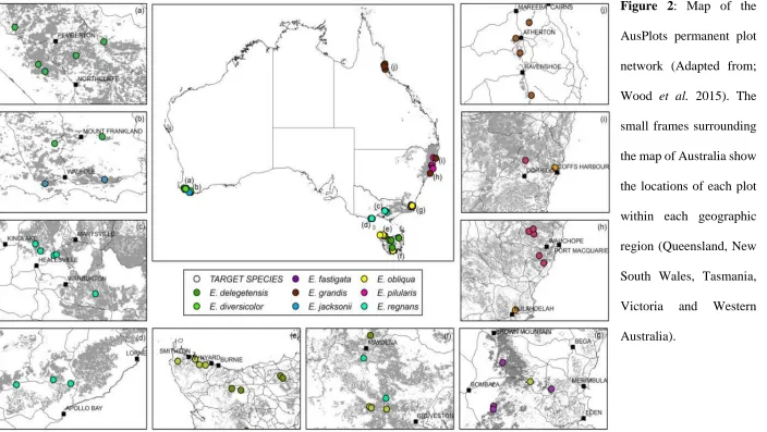
AusPlots permanent forest plot network

(30)

studies of tree locations, sizes, and species identity, based on the idea that the spatial pattern of trees might conserve the fingerprints of past, often hidden, processes (Wiegand and Moloney 2004; Perry et al. 2013).

(31)

[image:31.842.76.780.116.513.2]

(32)

[image:32.842.74.731.180.514.2]

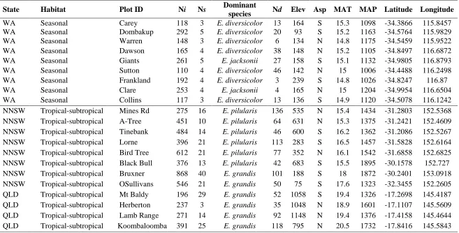
Table 1: Key ecological features in the AusPlots tall eucalypt forest network. Ni = number of individuals, Ns = number of species, Nd = number of standing dead trees, Elev = elevation, Asp = aspect, MAT = mean annual precipitation (mm), MAP = mean annual precipitation)

State Habitat Plot ID Ni Ns Dominant

species Nd Elev Asp MAT MAP Latitude Longitude

(33)

State Habitat Plot ID Ni Ns Dominant species Nd Elev Asp MAT MAP Latitude Longitude

(34)

Thesis aims

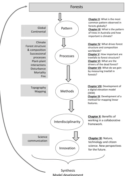
There are many gaps in knowledge and unsolved topics in forest ecology, that are centred on the importance of the processes underpinning observed spatial patterns. Furthermore, beyond description, there are relatively few applications of hypothesis- and process-driven (bottom-up) mechanistic models and frameworks to answer critical questions on the future of Australia’s tall-eucalypt forests: a biome under pressure from both global change and local anthropogenic pressures. Therefore, my thesis focuses on developing—for the first time—a comprehensive understanding of the structural and spatial processes that govern tall eucalypt forests across Australia, with the goal of deriving generalities that provide both a useful contribution to ecological theory, and practical benefits for the conservation of these spectacular Australian ecosystems (Fig. 3).

Overview of thesis chapters

:

(35)

(36)

[image:36.595.115.523.91.662.2]

Fig. 3: Overarching thesis structure and framework. The arrows show the flow of idea generation, and the natural sequence of research.

Forests

Pattern Processes Methods Interdisciplinarity Innovation Synthesis Model development

Chapter II: What is the most common pattern observed in forests globally?

Chapter III: What is the pattern of trees in Australia and how important is climate?

Chapter IV: What drives forest structure and composition worldwide?

Chapter V: How important are treefalls to forest structure? Chapter VI: What are the drivers of the dead forest? Chapter VII: What do we gain by measuring treefall in forests?

Chapter VIII: Development of a digital elevation model (DEM)

Chapter IX: Development of a method for mapping linear features.

Chapter X: Benefits of

working in a collaborative framework.

Chapter XI: Nature,

technology and citizen science. New perspectives for the future.

(37)

CHAPTER II

A GLOBAL SYNTHESIS OF

REPORTED SPATIAL PATTERNS

IN FORESTS

Studies on large tropical forest plots suggest that aggregation is a common pattern

for trees. However, despite the sophisticated tools available to analyze spatial

information, it remains unclear whether plot design and/or geographic location of

forest plots that report spatial information are globally cross-comparable. We

synthesized the spatially explicit forest-plot data from six continents, based on the 87

studies reporting explicit pattern statistics (either as community composites or for

individual species). From these, 264 unique forest plots, including >1,000 species

occurrences, were represented. Our analyses demonstrated that aggregation is not a

tropical peculiarity; it persists as the dominant pattern (over 65% of communities and

species) reported in forest-plots worldwide. However, our ability to synthesize

reported global pattern data and generalize across studies was confounded by

differences in the number of species analysed per plot, geographical bias across

continental forest areas, and methodological inconsistencies (in plot size and

(38)

place a strong emphasis on point-pattern statistics for characterizing spatial

structure. For these data are to be included in future meta-analyses, we recommend a

more standardized approach to reporting metrics, and coordination of the choice of

plot and tree size measured.

Introduction

he desire to improve understanding of forest dynamics and structuring has led to the widespread adoption of plot-based censuses of individual trees around the world (Anderson-Teixeira et al. 2015). These studies use a combination of static-pattern measurements and long-term monitoring to follow changes in tree distribution, carbon allocation, mortality etc., over time. The baseline data for these permanent plot networks is usually a ‘snap-shot’ study of tree locations of one or more species within the community, typically established with the underlying goal of deducing past processes from observable standing patterns (Perry et al. 2002; Wiegand and Moloney 2004). However, interpreting these instantaneous spatial data and linking it to time-dependent ecological processes is inferentially challenging (McIntire and Fajardo 2009), especially during periods of rapid environmental change. For instance, despite the availability of robust methods for analysing spatial point-patterns, there remains a wide range of simple to complex metrics and model outputs that are being reported (Velázquez et al. 2016). This has meant that, to date, few generalities or convincing syntheses have emerged on any reciprocal link between pattern and process in forest dynamics (Grimm et al. 2005).

(39)

Ideally, connecting an observed spatial pattern to a specific process should follow from a detailed plot-based analysis of local attributes such as topography, disturbance, and legacy effects (a ‘bottom up’ approach), although such studies are rare (Grimm et al.

(40)

(41)

Materials and methods

Spatial literature database

(42)

grouping aggregated and regular as a (non-random) “pattern” and contrasting this with randomness is provided in the Supplementary material Appendix 1; results were similar to the analysis with C and Ra alone. For those studies with multiple sampling dates, only the most recently reported data (community measurements) and spatial patterns were used, to avoid pseudo-replication of forest plots. We also crosschecked the literature to account for circumstances where different studies examined the same plots/forest communities; in these cases, each additional study was given the same ID number and assigned a letter. Taxa that were represented multiple times across different studies/communities (forest plots) were included within the data frame; however, subsampling approaches were applied in the statistical analysis in order to avoid pseudo-replication of species (described in detail below).

Community-level analyses

(43)

[image:43.595.115.526.84.393.2]

(44)

[image:44.842.114.788.214.474.2]

Table 1: Summary of the studies included in the research synthesis, by continent, reporting spatial patterns in forest plots. Key diagnostic variables were, total forested area (FAO Global Forest Resources Assessment; http://www.fao.org/forestry/fra), number of communities represented, number of communities with species pattern information, number of unique species, and number of species occurrences for which pattern information was available. The average plot size and most common tree size measured (minimum diameter at breast height), is also shown.

Africa Asia Australasia Europe North America South America

Forested area (000 ha) 674,419 592,512 191,384 1,005,001 678,961 883,850 Plots for which we have species pattern reported 16 31 19 58 57 19

Plots we should expect per area of forested land 33 29 10 50 34 44 Species occurrences for which pattern was analysed and

reported

40 450 66 146 247 73

Average number of species pattern reported per plot 3 15 3 3 4 4 Average plot size (ha) 4 16 0.4 1 2 8

Tree size measured >6 cm >1 cm All All & 10 cm >1 cm & >10 cm

(45)

Accounting for plot representation, geographic bias, and methodology

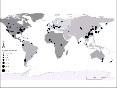
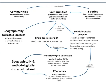
Although we considered the raw information in the subsequent modelling, for our main analyses we constructed two derived datasets; i) geographically corrected, and ii) a geographically and methodologically corrected dataset (Fig. 2). These datasets were prepared a priori, because the global distribution of species occurrences was uneven, with Asia being by far the most represented continent accounting for 44.0% of the 1022 species-level analyses, followed by North America with 24.2% (Table 1; Fig. 1); by contrast, there were few species occurrences in Australasia or Africa. When determining the number of communities/plots expected given the area of forested land on each continent and the number of communities for which pattern information has been reported, both Africa and South America are underrepresented (Table 1). We identified two important methodological decisions made by researchers – size (area in hectares, ha) of the monitored plot, and the minimum size (diameter at breast height, DBH) of trees selected for measurement. Plots in Asia were consistently larger than those on other continents, all species patterns in the plots were reported and smaller trees were typically included in the measurements (Table 1). To address all aims, we undertook analyses on the dataset that contained pattern information for individual species occurrences (i.e., data on species identity, dispersal vector, shade tolerance as well as methodological information; plot size, tree size measured, etc.).

(46)

(47)

[image:47.595.114.556.67.409.2]

(48)

We tested for geographic bias by: i) calculating the expected proportion of plots per continent, if they had been distributed according to continental forest area, and ii) repeatedly resampling (with replacement) the species-by-community data-set selecting a random bootstrapped selection of 198 rows (i.e., dimensions equal to the original number of communities with species information; Table 1), with the number of samples per continent being set equal to the expected proportions calculated in step i), repeated 10,000 times.

We were also interested in how a priori methodological choices might influence the spatial pattern observed in a plot. We tested this by first using a GLM to estimate the relationship between plot area (continuous), and minimum measured tree size (categorical, >1–2.5 cm [small] or >10–30 cm [large] DBH), and their interaction term, when regressed against pattern type (binomial: clustered or random). This fitted model was used to estimate the probability of no spatial structure (i.e., randomness) being observed for each individual species occurrence, given the plot size and smallest tree-size measured for that study. The expected probability was calculated for a ‘standardized’ plot of 1 ha area with all trees >1 cm DBH being measured. As a final step, if a random uniform deviate (U ~ [0,1]) was greater than the absolute difference in these observed and expected probabilities, then pattern type was left unchanged. Otherwise, random was switched to aggregated, or vice versa. This procedure was repeated for 10,000 resampled datasets, with inference made on the statistics of the bootstrapped data frames.

(49)

(50)

Results

Community-level predictors

Aggregation was the most prevalent pattern type observed for those studies of forest communities that reported second-order point-pattern summary statistics (60%), followed by randomness (18%). Relatively few studies reported regular or multiple [C, Re] pattern types (15%, and 8% of communities, respectively). Of the environmental variables, neither elevation nor climatic factors (saturated model: mean annual temperature, mean annual precipitation and actual evapotranspiration) explained much of the variance in the community spatial patterns (2% and 3% of the structural deviance explained, respectively), with AET as the best-supported model (w

= 0.3), explaining 6% deviance.

Species occurrence data: Evidence of methodological choice effect

(51)

a)

b)

(52)

error (SEM), derived from bootstrapping, and b) shows the effect of data correction on the proportion of aggregation when sampling using a single species per plot, compared to sampling of species occurrences (species may be represented more than once).

Influence of geographic bias and methodological choice on aggregation

Irrespective of the corrections applied to the raw data, aggregation was the most common pattern reported for all species occurrences and across all levels of ecological predictors (Fig. 3b). Overall, 74 – 79% of species occurrences were aggregated (based on sampling multiple species per plot), although after applying the geographic and methodological corrections, this proportion decreased to 68 – 77% (Fig. 3b). Indeed, when not correcting for plot representation, methodological choices or geographic bias the proportion of aggregated species was potentially overestimated by as much as 15% across all factors (Fig. 3b). Conversely, when considering only a single species to represent each forest plot (in any one bootstrap sample), the proportion of aggregation for the raw (sampled) dataset was reduced by 12%, to 64%, and changed little after geographic and methodological corrections were applied. Thus, more speciose plots— if all species are analysed using point-pattern statistics, and the result reported—will tend to skew the resulting global pattern-type observed (Fig 3b).

(53)

effect to be detected, the data must be adjusted to sample only a single representative species per plot, and ideally corrected for geographic biases and methodological choice (Fig. 4). Analysis of the fully-corrected data revealed that animal-dispersed species are less aggregated than those dispersed by wind (Fig. 4); this matches synthetic analyses of seed rain (Clark et al. 2005). Conversely, there was a tendency for higher proportions of aggregation for shade intolerant species (i.e., 2% deviance explained, Table 2a), but this effect was weak (marginally less supported than the null model, Table 2b).

(54)

a)

Model k -LogL wAICc %DE

Null 1 -50.53 0.413 (0.022-0.667) 0

ST 2 -49.86 0.277 (0.030-0.709) 1.4 (0.0-7.2)

DV 3 -48.99 0.188 (0.020-0.614) 3.1 (0.9-10.9)

ST+DV 4 -48.33 0.122 (0.018-0.454) 4.5 (0.4-13.7)

b)

Model k -LogL wAICc %DE

DV 3 -53.51 0.310 (0.023-0.724) 5.8 (0.6-15.7)

Null 1 -56.82 0.267 (0.001-0.650) 0

ST 2 -55.69 0.242 (0.003-0.744) 2.0 (0.0-8.4)

(55)

(56)

Discussion

Uniting pattern and process remains a central goal of spatial ecology (Levin 1992, Murrell et al. 2001; Murrell 2009). Recent increases in computational power and sophistication of statistical methods has led to a revolution in our capacity to model the patterns embedded in static spatial data, but a suite of complex (often stochastic and historically invisible) processes continue to confound our ability to use pattern information to infer process (Velázquez et al. 2016). Many ecological processes with strong spatial components, such as seed dispersal, facilitation and competition, can result in identifiable spatial patterns that conserve an imprint of past processes (Seidler and Plotkin 2006). However, similar patterns might also arise from quite different generating mechanisms, even within populations of the same species (Perry et al.

(57)

Influence of biases in plot location and study design

As hypothesised in aim (ii), methodological choices, when integrated globally, can affect the identification and generalisation of global trends in pattern type. The choice of plot size by researchers is driven in part by a need for sufficient sample sizes of trees (i.e., highly species rich communities with abundant stems [of all sizes] tend to not require large plots). These issues of methodological choice are problematic for research synthesises, because the areal extent over which a spatial analysis can be done, and the sample size of measured units, are tied inextricably to plot size and sampling intensity (Dale and Fortin 2014). Because a large proportion of global forest plots are smaller than one hectare, scale-dependent limitations will influence our ability to characterize pattern consistently, and therefore identify common processes (O'Neill et al. 1999; Dungan et al. 2002).

In this context, it is useful to think of a hierarchy of overlapping but scale-dependent forest processes. Fine-scale effects, in particular, tend to have a strong stochastic element that defies generalization. A mismatch between the characterisation of pattern (e.g. plot size or size of tree measured) and the operating scale of the underlying processes might therefore be common (but difficult to identify for a given study). Indeed, it was only through a synthesis of the global literature of many individual studies that this problem became apparent. Choosing measurement scales that best reflect the process or ecological question of interest could mitigate such issues – yet this is rarely done, both due to the sheer effort involved in setting up plots, and also because we often do not know which scales are important a priori (Wiens 1989; Hui

(58)

effects that interact with the stochastic drivers arising from the dominance of fine-scale influences (e.g., microclimate, topography) at the plot level.

Impact of methodological inconsistencies for linking pattern to process

For aim (iii), we tested two ecological traits (dispersal and shade-tolerance) that have been linked consistently to species-level spatial pattern, but we did not detect a strong influence on reported patterns. Reasons for this lack of explanatory power might include: uneven spread of trait variation across scales, overly coarse classification of spatial pattern, ontogenetic changes in trait expression, and unreported contextual information (e.g., site-specific attributes) that act to mask weaker ecological influences. Ontogenetic variability is possibly the most ecologically interesting, but least considered confounder when attempting to link broad ecological traits to observed patterns (Valladares and Niinemets 2008). For instance, if seedlings of a given species are shade-tolerant, but saplings or adults require exposure to direct sun, then the directionality of effects may cancel out. Furthermore, scale-dependent spatial heterogeneity across larger study areas might favour different axes of a trait, again acting to mask any signal when the entire plot is analysed for patterns. Evidence that microhabitat associations might shift between young (small) and old (large) trees further supports this argument (Comita et al. 2007).

(59)

processes (e.g., suitable soil chemistry, topography, facilitation) or reduced by interspecific competition. Such synergistic and antagonistic forces, acting collectively, might lead to a spectrum of patterns (or apparent randomness), depending on the relative strengths of the contributing processes (McIntire and Fajardo 2009). It is also likely that the datasets that we analysed, consisting of an overwhelming number of small-sized plots, compromised our ability to draw the effect of process out of the categorisation of pattern. This limitation could be overcome if future studies consistently report the raw metrics of spatial patterns (rather than simply testing conformity to a null model with limited information on scale dependency; Velázquez

et al. 2016), and by use of methods that link spatial-pattern analysis with stochastic, spatially explicit individual-based models (Grimm et al. 2005; May et al. 2015; May

et al. 2016).

(60)

differences, or because methodological choices (including the lack of representation of tropical species in Africa and South America, given their immense species count) make it difficult to confidently attribute differences in patterns across biomes solely to ecological drivers.

A notable feature of the forest-plot literature is ambiguity regarding whether the study design was testing a priori hypotheses about tree patterns, or if the data were analysed

post hoc. This decision is important because of the potential link between detection of spatial pattern and idiosyncrasies in study design (e.g., choice of plot location, size or species measured or other uncontrolled factors) (Gnonlonfoun et al. 2015). When we accounted for geographic bias and methodological choices regarding plot design, we were able to explain more variation in pattern type based on ecological traits. This outcome emphasizes the potential value of having a standard protocol that minimizes non-ecological influences on pattern detection (the CTFS plots published in Anderson-Teixeira et al. 2015) is a recent example of the move towards this). Few studies have addressed the influence of plot size or size of tree measured explicitly (Gnonlonfoun

et al. 2015) and the choice for any individual study is most often pragmatic. Another line of evidence for this effect comes from studies that reported measuring ‘all stems’. In these cases, propensity to aggregate more closely resembled that observed for plots where only large trees were included, suggesting that researchers attempted to measure all stems when densities were low enough to make this a feasible proposition. Our observation that large trees exhibit a more random spatial structure fits with the well-grounded theory of competition for space and resources, whereby ‘self-thinning’ acts to reduce stem density and so leave the remaining individuals less clustered (Li et al.

(61)

the CTFS network (Anderson-Teixeira et al. 2015), are best positioned to account simultaneously for joint effects of tree size, ecological determinants, and habitat heterogeneity (Shen et al. 2013), yet there are regrettably few of these in today’s global forest-plot network (Fig 1), and to date, published studies of reported pattern in the CTFS network are restricted to only a few of these plots.

Directions for future research

One way in which our top-down global synthesis of forest plot data could be improved is by incorporating more comprehensive and standardized site-specific information, such as abundance of individual species along with key geophysical and ecological factors (e.g., soil fertility, topography, local disturbance events, microclimate, etc.) (Ledo 2015). Furthermore, we urge future studies to examine more closely the ecological processes that underpin the general trend of aggregation seen across global forest plots, and just as importantly for contrast, the situations where randomness or regularity are apparent. The studies that seek these generalities should aim to characterize pattern quantitatively, and restrict future synthetic analysis to those studies that are methodologically comparable and geographically unbiased. One such approach may be to analyse the patterns of a consistent number of species using the CTFS standardized network (Anderson-Teixeira et al. 2015).

(62)

(63)

CHAPTER III

DRIVERS OF SPATIAL PATTERN,

DENSITY AND BASAL AREA IN

AUSTRALIAN TALL EUCALYPT

FORESTS

Forest are complex ecosystems, with their structure and composition determined by

multiple, often interacting, processes. Here we focus on two key drivers of forest

structure—climate and disturbance—using a recently established network of 48 ×

1-hectare censused plots spanning the Australian tall eucalypt forest estate. Using

spatial point pattern analysis, we find that aggregation is the dominant spatial pattern

at both the community- and species-level. Eucalypts showed clumped patterns across

62% of the plots and dominated the total basal area (83% average within the plot).

The mid- to understory non-eucalypts were also mostly aggregated (in 85% of plots),

but these dominated total tree density (85%, with many smaller stems) rather than

basal area. We used generalized linear modelling to determine the predictors of this

spatial patterning, as well as plot-level density and basal area (surrogates of

long-term productivity). Biotic variables best explained community spatial patterns (15%

(64)

dominant-species patterns (21.3%). Climate was a strong predictor of non-eucalypt

basal area and density, and eucalypt basal area (but not density), consistently

explaining >40% of the deviance in these variables. This study demonstrates the

importance of climate and disturbance in driving the structure of the tall eucalypt

forests of Australia.

Introduction

patial and abundance patterns are imprinted with the processes that have shaped forest structure and dynamics through time, which analysis of the statistics of point locations can reveal. As a consequence, spatial point-pattern analysis has become a standard tool for ecological studies of coordinate data of trees in forest communities worldwide (Velázquez et al. 2016). For example, aggregated (clumped) patterns in a forest community might indicate that a group of species has regenerated in a canopy-gap following a disturbance event. Over time, competition between immediate neighbours will ensue, with density-dependent mortality thinning out the clumps, potentially leading to the formation of regular spatial patterns as canopy trees reach maturity (Moeur 1997; Getzin et al. 2008). In addition to plant-plant interactions, spatial patterning can be driven by environmental heterogeneity, both within sites (e.g., clustering along waterlines, specific soil types, or due to local topographic variation) and across sites (e.g., due to climatic influences) (Fangliang et al. 1997). Such relationships are of interest, because ecologists are still constrained in their ability to predict spatial structures manifest in the same forest type over broad geographic and climatic ranges.

(65)

Beyond the spatial distribution of individual trees, the long-term productivity of forest ecosystems (as measured by standing patterns of biomass and structure, such as density or basal area) will also be shaped by top-down climatic conditions (e.g., available energy, precipitation or seasonal extremes), biogeographic factors (e.g., historical refugia, nutrient content of soils), and functional traits of species (e.g., shade tolerance or dispersal vector) (Paquette and Messier 2011; Reich et al. 2014). However, it is difficult to generalise across studies of different forests, due both to uncontrolled variation such as methodological choice (such as plot size or field methods) and forest type, along with limits on the coverage of samples that span wide continental scales. To date, studies linking spatial patterns and structure to inferred processes include forests of the Afrotropics (e.g., Friis 1992), boreal forests of Minnesota (Frelich and Reich 1995), and Picea-Fagus forests of East-Central Europe (Szwagrzyk and Czerwczak 1993), with most research concentrated in tropical regions (due in part to the establishment of multiple large 25–52 ha plots in tropical countries (Condit et al. 2000; Wang et al. 2010; Wang et al. 2011; Anderson-Teixeira et al.

2015).

(66)

perhaps because they have been considered broadly equivalent to temperate broadleaf biomes from the northern hemisphere.

(67)

(68)

Materials and methods

Spatial point pattern analysis - Univariate

The underlying spatial pattern of communities (pooled over species) and species (> 20 individuals per plot) was determined using spatial point pattern analysis. We used the pair correlation function (PCF) to describe patterns and the linearisation and variance-stabilising correction of the K-function (Ripley’s K) L(r) to explore how well alternative point-process models characterise them (following Perry et al. 2008). Strength of departure from the null model of complete spatial randomness (CSR) was determined using the model fit (u rank), Clarke and Evans statistic and Donnelly summary statistic, and was aided by visual inspection of the diagnostic plots (see Spatial null models section below and; Wiegand and Moloney 2013). Under CSR, L(r) = 0; aggregate patterns show L(r) > 0 and regular patterns L(r) < 0. The edge corrections described by Goreaud and Pélissier (1999) were used, and we calculated L(r) and g(r) at 0.1m intervals up to a distance of 25m.

Spatial null models

(69)

of high light or nutrient availability) factors. To characterise the observed spatial patterns, and distinguish between the two types of aggregation – first-order and second-order, we generated simulation envelopes using three alternative null models; the Homogeneous Poisson process (HPP), Inhomogeneous Poisson process (IPP) and the Poisson Cluster process (PCP). For further details on the null models and how they distinguish between first- and second- order aggregation, see Perry et al. (2008). To assess model fit, simulation envelopes were calculated at alpha = 0.01 based on 499 Monte Carlo simulations. To assess deviation from the various null and alternative models we used the Cramer von Mises (CvM) statistic, which is the sum of the squared deviation of the observed from the expected across all distances (Perry et al. 2006); for the HPP, IPP and PCP we used the mean of the Monte Carlo simulations as the expected value (Perry 2006; Perry et al. 2008). The R library spatstat v1.50 (Baddeley and Turner 2005) was used for all spatial analyses using R v3.4.0 (R Core Team, 2017).

Predictors of pattern, density and basal area

(70)

(71)

(72)

Ecological Questions/hypotheses Analyses

Spatial analysis - Univariate

Community (1 ha plots – all stems)

1. Do plots in the same forest type (tall

eucalypt forests) show the same pattern

type?

2. Is the observed aggregation best described

by environmental heterogeneity across

Australia, or interactions between individual

trees?

Species (>30 individuals)

1. What is the most prevalent pattern type for

species across Australia in the tall eucalypt

forests? a) Across each habitat? b) Between

guilds (scl, rf, euc)?

2. Is the observed aggregation best described

by environmental heterogeneity, or

interactions between individual trees of the

same species?

Climatic drivers of forest structure

1. Is climate an important predictor of

eucalypt and non-eucalypt density and basal

area and what are their relationships?

Spatial point pattern analysis, test against departure from

complete spatial randomness (CSR).

Evaluate departure from CSR using two alternative models;

inhomogeneous Poisson process (first order aggregation) and a

Thomas cluster process (second-order aggregation). Assess

model fit using Clarke-Evans, and Donnelly statistic, visual

examination of graphics and (u + rank).

Group by guild (i.e., eucalypt, sclerophyllous or rainforest

species) and evaluate pattern-type (departure from CSR). Run a

GLM testing the influence of guild as a predictor of species

patterns.

Evaluate departure from CSR using two alternative models;

inhomogeneous Poisson process (first order aggregation) and a

Thomas cluster process (second-order aggregation). Assess

model fit using Clarke-Evans, and Donnelly statistic, visual

examination of graphics and (u + rank).

Generalized linear modelling (GLM) approach. All subsets of

climate models tested (after checking for correlation). Best

climate model for each dependent variable determined using

wAICc and deviance explained. Report deviance explained,

(73)

Results

Spatial patterns – communities (all stems)

Aggregation was the most common pattern type across the tall eucalypt forest plots of Australia (62% aggregated, 15% random, and 23% regular). Of the 62% of plots that were aggregated at distances of up to 20 m, there were distinct groupings in the percentage (%) of communities exhibiting aggregation across habitat types (e.g., seasonal and temperate 67%, and tropical-subtropical 42%). Tropical-subtropical habitats showed the highest fraction of regular and random plots (33% and 25% respectively), while temperate and seasonal were consistently lower at 22% and 11%. Half of communities conformed to a homogeneous Poisson (CSR) model, whereas 23% fit best to an IH, and 27% to a CP.

Predictors of community and species

patterns

1. Are spatial patterns best described by

biotic (average tree size, total basal area,

number of species), abiotic (MAT, Trange,

MT_DQ, MAP, PDM, PCQ), or habitat

(temperate, seasonal, tropical-subtropical)

for:

a) Community (all stems) spatial patterns

and

b) Dominant species patterns

variable. a) Linear model of a priori combinations of total

density and total basal area with eucalypt and non-eucalypt

density and basal area.

Generalized linear modelling (GLM)

Biotic saturated model vs. abiotic saturated model (% deviance

explained) compare to biogeographic predictor (habitat). Rank

models by wAICc. Report deviance explained and fit for best

(74)

Fig. 2: Example of three different types of community-level patterns (aggregation [a], randomness [b], regular [c]) and their corresponding L(r) functions, confidence envelopes (grey shading), at the α = 0.01 level using an inhomogeneous Poisson

model. The column of figures on the left show the positions of all stems in the 1 hectare plot.

a) Weld

b) Carey

(75)

Spatial patterns – species and species occurrences

There were 153 species occurrences across the 48 × 1-hectare eucalypt-dominated AusPlots, drawn from a pool of 55 unique species of tree >10 cm DBH. The most common pattern for all species occurrences was aggregation (73%), followed by randomness (20%), with few exhibiting regularity (7%). Aggregation was most often observed at shorter distances (45%0–5m and 25%>5m–20m of total species, respectively), with regular patterns also following this trend (7%0–5m vs. 4%>5m–20m, respectively).

There were consistent species patterns across habitat zones in Australia – tropical-subtropical areas had the highest percentage of aggregated species (77%), followed by cool-temperate (73%) and seasonal (65%). Regularity was rare for all species occurrences, being only detected in seasonal, and cool temperate habitats (11% and 8% respectively). When grouping species occurrences by guild, sclerophyll and rainforest species (non-eucalypts) were indistinguishable in pattern type, with 84% and 82% aggregated respectively, compared to eucalypts of which only 60% were aggregated (see SI results 2a). More non-eucalypts were aggregated than eucalypts across all distances (Z0–20m = 3.05, SE0–20m = 0.43; SI results 2b).

Predictors of eucalypt and non-eucalypt density and basal area

(76)

[image:76.595.113.524.401.664.2]

MT_DQ and PCQ for eucalypt basal area (Table 2). The direction of the effects is crucial for understanding the dynamics of these two groups, as both the slope and direction of their response to these predictors differs (Fig. 3). The basal area and density of eucalypts is higher when MT_DQ is low and PCQ is high. Conversely, greater non-eucalypt density and basal area are associated with high annual rainfall and narrow temperature range (Fig. 3).

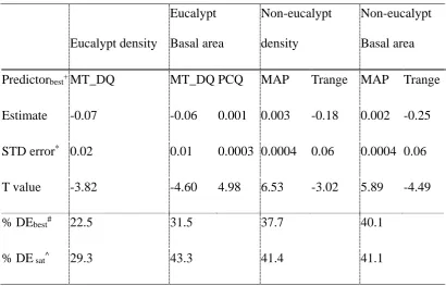
Table 2: Summary statistics of the best climatic-based generalized linear models for predicting density and biomass (basal area) of Australian eucalypt forest plots.

Footnotes: *_{Standard error.}#_{Deviance explained by the AIC}

c best model (as shown in the ‘Predictorbest’

column). ^_{Deviance explained by the saturated model (containing all climatic variables in an additive}

model).

Eucalypt density

Eucalypt Basal area

Non-eucalypt density

Non-eucalypt Basal area Predictorbest+ MT_DQ MT_DQ PCQ MAP Trange MAP Trange Estimate -0.07 -0.06 0.001 0.003 -0.18 0.002 -0.25 STD error*_0.02 _0.01 _{0.0003 0.0004 0.06} _{0.0004 0.06} T value -3.82 -4.60 4.98 6.53 -3.02 5.89 -4.49

% DEbest# 22.5 31.5 37.7 40.1

(77)

Fig. 3: Relationship between density (number of individuals), basal area (m2 ha-1) and climatic variables for both guilds (eucalypt and non-eucalypt).

Community density across the 48 plots is driven by the non-eucalypts (because these contain many more individual trees), whereas total basal area is mostly determined by the eucalypts, these being the dominant large canopy trees (Figs. 4 a, b). Non-eucalypt basal area is highest when fewer eucalypts are present, and as eucalypt density increases the contribution of non-eucalypt basal area diminishes (Fig. 4 c). There is no relationship between eucalypt and non-eucalypt basal area (r = 0.014, p = 0.925), nor for density (r = 0.02, p = 0.893). There is, however, a strong positive linear correlation

MT DQ MAP Trange

Trange MAP MT_DQ PCQ Non-eucalypt Eucalypt De ns ity (num be r o f i ndi vi dua ls Bas al ar ea ( cm

(78)

between density and basal area of non-eucalypts (r = 0.794, p < 0.001), but it is only weak for eucalypts (r = 0.282, p = 0.052).

Fig. 4: Drivers of total density and total basal area for the 48 Australian 1ha plots. a) relationship between total basal area and eucalypt basal area, b) relationship between total density and non-eucalypt density and c) relationship between the percentage contribution of basal area by both species and the percentage contribution of eucalypt density to total density.

0 0.2 0.4 0.6 0.8 1 1.2

0 0.1 0.2 0.3 0.4 0.5 0.6 0.7 0.8 0.9 1

% c ont ri but ion of ba sa l ar ea by gui ld

% contribution of eucalpyt density to total density non-euc euc

R² = 0.8508

0 100 200 300 400 500 600 700 800 900

0 500 1000 1500

T ot al de ns it y ( no. i ndi vi dua ls ) Non-eucalpyt density

R² = 0.8357

0 10 20 30 40 50 60 70 80 90

0 50 100 150

T o tal b as al ar ea (m 2ha -1)

Eucalypt basal area (m2_ha-1₎

a) b)

(79)

Predictors of community and species patterns

Communities

Biogeography (biome) was not a useful predictor of community spatial patterns in Australian tall eucalypt forests (%DE = 1.6 for the saturated model). The biotic model explained slightly less variance (%DE = 15.6) in pattern type than the abiotic model (%DE = 16.4). A combination of average tree size and number of species was the most parsimonious simplified model overall (wAICc = 0.52, %DE = 15.0), suggesting a tendency towards aggregation with smaller tree sizes and fewer species present in a forest plot. The best abiotic predictor(s) was a single term: temperature range (wAICc = 0.119, %DE = 6.5).

Dominant eucalypt patterns

(80)

(81)

Discussion

The underlying spatial patterns of the tall eucalypt forest system, as characterised by the new 48 one-hectare AusPlots network, support the global prediction that aggregation is the most common pattern in communities, particularly at local scales (Plotkin et al. 2002; Zhang et al. 2012). Individual species in the AusPlots also exhibited aggregated patterns (particularly at short distances, 0–5 m, and for the smaller, non-eucalypt species). Traits such as shade-tolerance and dispersal vector have been shown to be highly correlated with pattern-type across multiple ecozones worldwide (Seidler and Plotkin 2006; Wang et al. 2010). However, these were not informative on spatial pattern for any individual species in this study, perhaps due to the emergent habit of the dominant eucalypt species (Attiwill 1994), and because structuring of these forests is driven by frequent disturbance and climatic variation, which are not species specific, as distinct from filtering via individual species traits (Bonan 2008).

(82)

thrived with narrower temperature ranges (indicating avoidance of temperature extremes), eucalypt density and basal area were higher in cold-dry conditions. Climatic variables were poor predictors of basal area for eucalypts, perhaps because local adaptations were smeared out across a continental scale. The differences observed here between eucalypts and other species suggest a decoupling of the guilds. But if climate is not a strong predictor of eucalypt density and basal area, what is their main driver?

(83)