GPS derived strain rates on an active ice shelf rift

GPS-DERIVED STRAIN RATES ON AN ACTIVE ICE SHELF RIFT

V. Janssen1_{, R. Coleman}1,2,3_{and J.N. Bassis}4

1 _{University of Tasmania, Hobart, Australia}

2 _{CSIRO Marine and Atmospheric Research, Hobart, Australia}

3 _{Antarctic Climate and Ecosystems Co-operative Research Centre, Hobart, Australia} 4 _{Scripps Institution of Oceanography, La Jolla, California, USA}

ABSTRACT

Ice shelves are important components of the Antarctic ice sheet due to their ice-ocean-atmosphere interface and vulnerability to global increases (or decreases) in atmospheric and oceanic temperatures. The development of rifts, which are fractures that penetrate through the entire ice shelf thickness, precede large tabular iceberg detachment and can lead to ice shelf break-up. Changes in strain rates on an active propagating rift system on the Amery Ice Shelf, East Antarctica are determined using in-situ Global Positioning System (GPS) measurements. Results for the 2002/03 Antarctic summer period (Dec-Feb) confirm previous observations by [2] that rift propagation occurs in episodic bursts separated by several days. Transverse-to-flow (i.e. parallel-to-rift) strain rates exceed longitudinal-to-flow (i.e. normal-to-rift) rates by up to a factor of 5 and maximum principal strain rates around the rift tip vary from 12 to 21 [x 10-3_{/yr]. A rotation in the direction of the principal strain is evident around the} rift tip, indicatinga change in the mechanics of rift fracture. It is demonstrated that cumulative sum analysis [12], obtained by differencing a pair of residual baseline time series situated approximately normal and parallel to the rift, is an effective method to detect small baseline length changes.

KEYWORDS: GPS. Strain rates. Ice shelf rifting. Amery Ice Shelf.

INTRODUCTION

Ice shelves are sensitive components of the Antarctic ice sheet due to their natural cycle of mass loss, primarily through iceberg calving and basal melt, making them important indicators of climate change [18]. With the vast amount of ice stored in the Antarctic ice sheet, any increased mass loss can have significant effects on the water budget, and hence major implications for global sea level and ocean currents which, in turn, can affect global climate [20]. Furthermore, the very presence of ice shelves affects the continental flow of the grounded ice sheet towards the coast via the ice shelf systems by shielding these systems from a potential major retreat [8]. The continuing temperature increase across the entire Antarctic continent [24] and the recent retreat and disintegration of several ice shelves [22], [23] have emphasized the need for us to better understand the mechanisms that are responsible for iceberg calving.

the Antarctic and Greenland ice sheets are losing mass, resulting in a contribution of about 0.42 mm per year to global sea level for the period 1993-2003.

Several studies have investigated ice shelf rift propagation using different techniques including satellite imagery, InSAR, satellite altimetry, GPS and seismic observations. These studies have revealed that rift propagation is driven primarily by the internal glaciological stress of the ice shelf and occurs in episodic bursts [2], [15]. Propagation rates on the Amery Ice Shelf are seasonally dependent with significantly higher rates in the summer period [10] and the collection of ice and snow trapped inside the rift (often called ice mélange) may potentially play a role in the rifting process [9], [17]. Previous analysis of rift propagation on the Amery Ice Shelf was investigated by [2] using 46 days of GPS data, processed in kinematic mode, and incorporating seismic observations to detect “icequakes”. It was revealed that propagation occurs in episodic bursts lasting about 4 hours, with bursts separated by 10-24 days. The investigation of nearby automatic weather station data and tidal amplitudes seen in the GPS data showed that these bursts are not directly caused by winds or tides, suggesting that the primary driving force is the glaciological stress of the ice shelf. This present study is based on the same GPS dataset but has a different focus. The aforementioned studies have concentrated on the dynamics of rift propagation rather than closely investigating the strain rate in the vicinity of the rift tip. We also use different GPS analysis techniques to those of [2].

Knowledge of strain at different locations on an ice shelf is of significant importance since it is a determining factor in ice dynamics, especially in initiating ice shelf break-up [11]. Vertical strain is an important parameter in determining the rate of ice shelf thickness change and bottom melt rates.

Changes in the climatic conditions on the ice shelf, e.g. caused by an increase in ocean or atmospheric temperature or a change in snow accumulation, may be reflected in strain rate changes. Strain rates can be determined by measuring changes in distances between several points, usually arranged in triangles or quadrilaterals, over time. One-dimensional strain is defined in terms of an extension or contraction of a line, while shear strain is defined in relation to the angular change between two perpendicular lines (i.e. two-dimensional). If the vertical component is also considered, a three-dimensional strain model is obtained [3]. Alternatively, vertical strain can generally be calculated through the continuity equation [5]. However, this paper concentrates on horizontal (2-d) strain rates.

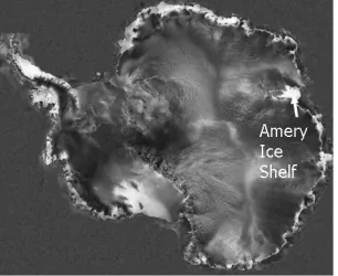
We investigate the horizontal strain rate distribution around an active rift system, known as the “Loose Tooth”, on the Amery Ice Shelf, East Antarctica (Fig. 1). Results based on data collected at six GPS sites during the Antarctic summer of 2002/03 are presented.

STUDY AREA AND OBSERVATIONS

The Amery Ice Shelf (AIS) is the largest ice shelf in East Antarctica, draining continental ice from an area of more than one million square kilometres [1] through a section of coastline that represents approximately 1.7% of the total continental circumference [6]. The Loose Tooth rift system is located at the front of the AIS and encompasses an area of about 30 km by 30 km, an area that will likely calve and produce a large iceberg in the future. The Loose Tooth rift system consists of two longitudinal-to-flow rifts (denoted L1 and L2) and two transverse-to-flow rifts (denoted T1 and T2) (Fig. 2). Both rifts T1 and T2 occur in the transition zone where transverse-to-flow strain rates begin to exceed longitudinal-to-flow strain rates [28]. In this region the ice shelf is ~400 m thick and the ice shelf flow is approximately 3 m/day (1.1 km/year) in a north-easterly direction [2]. The T2 tip advances currently at about 4 m/day [10]. Evidence has been presented that rift propagation occurs in episodic bursts and is primarily driven by the internal glaciological stress of the ice shelf, rather than initiated by winds or ocean tides [2].

Young and Hyland [28] determined velocity and horizontal strain rates over the entire Amery Ice Shelf from InSAR measurements acquired 24 days apart. The InSAR resolution, however, is not sufficient to investigate spatial changes in strain rates in close proximity to a rift, nor can these data be used to investigate required temporal changes in strain rates. If available, these data could be used for comparison to the results of this study. However, problems were encountered with the coherence of InSAR images in the Loose Tooth area [28], prohibiting this comparison.

The GPS network consisted of six stations spanning the area immediately behind (LTS1, LTS2), in front (LTN3, LTN2) and either side (LTN1, LTS3) of the T2 rift tip (Fig. 2). The equipment used was a combination of Ashtech and Leica dual-frequency GPS receivers powered by batteries and solar panels, collecting data at 30 second epochs for 46 days.

Fig. 2. LANDSAT 7 ETM image of the Loose Tooth rift system acquired on 2 March 2003 and location of GPS stations around the tip of T2 overlaid on a LANDSAT 7 image acquired on 7 November 2002. Adapted from [2].

crevasse, however it was not evident that this affected the results presented here in any obvious way.

DATA PROCESSING AND METHODOLOGY

The GPS data were processed in daily (24-hr) sessions using the Leica SKI-Pro version 2.0 software. The elevation mask was set to 10° and IGS precise ephemerides were used. Full antenna phase centre variation models were applied, accounting for corrections depending on the azimuth and elevation of each satellite. Since the L3 ionospheric-free linear combination was deemed not reliable over the relatively short baselines in this network (distances of 1-5 km), an ionosphere model was computed from the reference station data of each baseline. The Saastamoinen model was applied to account for the tropospheric delay.

Five triangles were formed in order to investigate strain rates as a function of geometry relative to the propagating rift tip. Two triangles were located entirely on the northern and southern side of the rift respectively, while the others straddled the rift (see Fig. 2). In addition, all baselines were examined individually to verify data integrity and to study the time series for systematic variations.

Since the distances between sites are short (generally less than 5 km) and relative measurements between points are used, a ‘vertically-stationary’ (or quasi-stationary) ice shelf can be assumed where differential tidal motion and atmospheric variations between sites are assumed negligible, i.e. common systematic effects are removed. In reality, in this region the ice shelf is moving at approximately 3 m/day in a north-easterly direction [2], [28] and experiences a vertical, tidal motion with a peak-to-peak amplitude of approximately 1-2 m [16], [29]. However, because the size of the network is small compared to the wavelength of the tide, the differential motion due to the tide between sites is small. This is confirmed by the AIS tide model generated by [21], which does not show any significant differences in the tidal signal between stations over such short distances (less than mm over the network). With the underlying uniform motion of the ice shelf across the network removed, any remaining relative movements between network points can then be interpreted as strain. The determination of baseline distances situated normal to the rift can be used to infer opening rates of the rift as the rift tip passes through the GPS network.

The output of the SKI-Pro processing was a set of daily baselines in terms of ITRF2000 global Cartesian coordinate differences. These coordinate differences were then transformed into a local north-east-up (NEU) coordinate system and aligned (rotated) with the local flow direction of the AIS. The local flow direction was inferred from satellite imagery to be 44° and which, in this case, is predominantly orthogonal to the rift propagation direction.

Strains and strain rates

Strains were determined in two different ways. Firstly, the daily changes in the longitudinal-to-flow (i.e. normal-to-rift) and transverse-to-flow (i.e. parallel-to-rift) components of each baseline could easily be converted into extensions/contractions in these directions since the coordinate axes were already aligned with the desired direction. This resulted in longitudinal and transverse strains for each baseline, which were then converted into strain rates by determining the change in strain over time. The second approach is based on the difference of (horizontal) distance observations and was employed for all five triangles formed. The procedure is outlined by [4] and the basic equations used are summarised below.

2 2

/ = cos + sin + sin 2

PQ PQ xx PQ yy PQ xy PQ

∆S S ε β ε β ε β ₍₁₎

where ∆SPQ is the change of the (horizontal) baseline length SPQ, βPQ is the bearing of

the baseline in the Cartesian coordinate system (x,y), εxx and εyy are the extensions in the x and y directions respectively, and εxy is the shear strain component. In this study, the x axis represents the longitudinal-to-flow (i.e. normal-to-rift) direction while the y

axis refers to the transverse-to-flow (i.e. parallel-to-rift) direction.

Differencing baseline observations (l1 and l2) between two epochs yields the

following set of equations [4]:

(

)

2− 1 = s s = ε ε εxx yy xy

l l Au u (2)

where A is the design matrix based on equation (1). For an over-determined system of observation equations, the least-squares solution for the strain components us is then

given by:

(

)

(

)

(

)

∆ ∆ with ∆

s 2 1 P

− −

= − =

u A P A A P l l Q A P A (3)

where P∆ is the weight matrix of the observation differences, calculated using the law

of the propagation of variances after scaling the SKI-Pro output in order to obtain realistic estimates (a-priori variances were scaled by 400), and QP is the

variance-covariance matrix of the resulting strain estimates which yields precision estimates of the results.

The resulting strain parameters can then be converted to the widely used engineering shear strains γ1 and γ2 [7]:

and 2

1 yy xx 2 xy

γ =ε −ε γ = ε (4)

where γ1 refers to the engineering shear across a plane normal to the x-y plane and bisecting the x-y axes, and γ2 represents the shear across a plane parallel to the y axis. The maximum shear strain γ is then determined by:

2 2

1 2

γ= γ +γ (5)

The maximum and minimum principal strains and their respective azimuths are obtained by [27]:

(

)

(

)

max min

1 1

and

2 2

= xx+ yy+ = xx+ yy−

e ε ε γ e ε ε γ ₍₆₎

1

max min max

1

tan and

2 2

2

1

γ π

α α α

γ

−  

= _{ } = ±

−

  (7)

In the present study, the daily strain estimates were used to determine six weekly strain values for the five triangles formed. Strain rates were computed from the weekly strains.

Baseline change detection using cumulative sums

decades. The reader is referred to [19] for a discussion on geodetic applications of CUSUM charts. If there are no changes in the mean of the time series, the data are considered random and the CUSUM chart displays a flat straight line. An upward slope indicates a period where values are above the mean, while a downward slope indicates a period where values are below the mean. The technique proposed by [12] forms the difference of two baselines that share a common site in order to reduce common systematic errors and thereby allow the detection of small changes, which would otherwise be buried within the observation noise. In practice, after removing any linear trends and periodic variations in the baseline time series, the resulting residuals are used as quasi-observations for further analysis.

CUSUM charts were generated for the baseline time series of LTS3-LTN1 and LTN1-LTN3 and then differenced for each epoch to reduce the influence of any remaining unmodelled systematic errors. If the two baselines run approximately parallel and perpendicular to the expected deformation, any hidden changes in the time series can be detected, although it should be noted that these changes will be reduced in magnitude as any common signal is removed in the difference. Any sudden change in the slope of the CUSUM indicates a shift in the mean, i.e. a jump in the baseline length. With the orientation of this baseline pair, orthogonal and parallel to the rift, we should detect any rift opening.

RESULTSAND DISCUSSION

The following sections present the results obtained and discuss the findings in terms of rift propagation, strain rates determined with the two methods and baseline change detection using cumulative sums.

Rift propagation

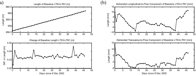
The shortest baseline spanning the rift, LTS3-LTN1, increases in baseline length by approximately 35 mm/day and exhibits three jumps of ~10 mm on days 1, 13 and 38 (Fig. 3). The day numbers are relative to the start of processing (8 Dec 2002), i.e. day 1 corresponds to 9 Dec, etc.

0 5 10 15 20 25 30 35 40 45 50 958.5

959 959.5 960

960.5 Length of Baseline LTS3-LTN1 [m]

Lengt

h [

m

]

0 5 10 15 20 25 30 35 40 45 50 0.02

0.03 0.04

0.05 Change of Baseline Length LTS3-LTN1 [m]

Days since 8 Dec 2002

D iff . i n L engt h [m ]

0 5 10 15 20 25 30 35 40 45 50 -10

-5 0 5 10

15Detrended Longitudinal-to-Flow Component of Baseline LTS3-LTN1 [mm]

Len gt h [ m m ]

0 5 10 15 20 25 30 35 40 45 50 -5

0 5 10

15 Detrended Transverse-to-Flow Component of Baseline LTS3-LTN1 [mm]

Days since 8 Dec 2002

Leng th [ m m ]

Fig. 3. (a) Length of baseline LTS3-LTN1 and its change over time, and (b) detrended longitudinal-to-flow and transverse-to-flow components.

Three jumps are clearly visible in the daily change of the baseline length and the detrended longitudinal-to-flow (i.e. normal-to-rift) component of the baseline. Although the transverse-to-flow (i.e. parallel-to-rift) component does indicate two of these jumps on days 13 and 38 (Fig. 3b), these are too small to be deemed significant – not surprisingly since the baseline is closely aligned with the longitudinal-to-flow

direction. The large ‘dip’ visible between day 0 and day 1 in Figure 3b may seem peculiar upon first inspection. This is an artefact that can be explained by the fact that data collection on the first day of the survey (i.e. day 0) started at ~13.00h UTC on 8 Dec, hence covering only the second half of the UTC day. When compared with the other daily solutions which are based on 24 hours of data to compute baseline components, it is clear that the resulting difference between days is smaller than usual because the motion that occurred in the first half of the day is not considered (evident in the larger upward jump in Figure 3a). This has been confirmed by processing 12-hour solutions for the first 7 days.

The results presented here confirm the findings of [2], showing that rift propagation exhibits an episodic behaviour with bursts of about 10 mm magnitude separated by several (10-25) days. These bursts are not evident in the longer baselines, primarily due to the increased noise levels that prevent detection of this small amplitude signal. At the rift tip, an opening rate of 35 mm/day over the Antarctic summer period is evident.

Strain rates derived from changes in baseline components (first method)

For all baselines, the daily changes in the baseline components were converted to yearly strain rates and a 5-day running mean filter was applied to the time series. Table 1 shows the magnitude of changes in baseline length, longitudinal-to-flow (flowL) and transverse-to-flow (flowT) components and ellipsoidal height difference (corrected for earth curvature) over 46 days. The resulting mean strain rates and their standard deviations are shown in Table 2.

Table 1. Differences in baseline components over 46 days (first method)

Baseline L [km] ∆L [m] ∆flowL [m] ∆flowT [m] ∆hell. [m]

LTN1-LTN2 1.9 +1.43 +0.97 +2.71 -0.03

LTN1-LTN3 2.0 +2.77 +1.94 +2.45 +0.05

LTN2-LTN3 2.8 +2.26 +2.93 -0.25 +0.07

LTS1-LTN1 4.1 +9.37 +1.40 +9.31 -0.09

LTS1-LTN2 4.9 +11.85 +2.35 +12.03 -0.13

LTS1-LTS2 2.8 +2.35 +0.92 +2.97 -0.02

LTS1-LTS3 4.0 +7.59 -0.07 +7.73 -0.08

LTS2-LTS3 3.0 +4.49 +0.99 +4.77 -0.10

LTS3-LTN1 1.0 +1.57 +1.34 +1.59 +0.01

LTS3-LTN3 2.2 +3.70 -0.60 +4.01 +0.03

Table 2. Strain rates determined from baseline components (first method)

Baseline L [km] Longitudinal strain

rate [10-3_/yr] Transverse strain _{rate [10}-3_/yr]

LTN1-LTN2 1.9 4.0 ± 0.1 63.7 ± 1.7

LTN1-LTN3 2.0 42.3 ± 0.4 10.2 ± 0.2

LTN2-LTN3 2.8 10.2 ± 0.2 -1.2 ± 0.1

LTS1-LTN1 4.1 49.8 ± 3.3 18.5 ± 0.8

LTS1-LTN2 4.9 8.8 ± 0.5 21.9 ± 0.6

LTS1-LTS2 2.8 3.1 ± 0.1 16.0 ± 0.5

LTS1-LTS3 4.0 -0.7 ± 0.4 15.9 ± 0.7

LTS2-LTS3 3.0 4.8 ± 0.2 15.8 ± 0.4

LTS3-LTN1 1.0 11.4 ± 0.6 85.0 ± 0.9

LTS3-LTN3 2.2 -8.4 ± 0.4 15.5 ± 0.2

both horizontal baseline components are of the same order, which can be explained by the rift opening in flowL direction. Changes in the ellipsoidal height differences are very small and not of interest in this study.

It is evident from Table 2 that transverse-to-flow strain rates are generally greater than longitudinal-to-flow strain rates, confirming the general trend shown in [28]. For baselines aligned with either the longitudinal-to-flow or the transverse-to-flow direction, the strain rates normal to this direction appear to be uncharacteristically large, which can be explained by the small coordinate component in this direction being vulnerable to variations caused by measurement noise. This translates into large strain rates that cannot be accepted as being representative of the true conditions. However, as discussed below, the strain rates obtained in the direction of the baselines have been found to be reliable.

Strain rates derived from baseline lengths and triangles (second method)

In order to investigate the distribution of strain rates as a function of geometry relative to the propagating rift, five triangles were formed and six weekly strain rate estimates were obtained based on the daily baseline lengths observed. Figure 4 shows the weekly estimates for the maximum and minimum principal strain rates as well as the azimuth of the maximum principal strain. The mean values for each parameter are also indicated. It can be seen that the weekly solutions are consistent. The largest variation is evident in triangle LTS1-LTN1-LTN2, which contains two relatively long baselines of the network.

Fig. 4. Weekly estimates of maximum and minimum principal strain rate and the azimuth of the maximum principal strain for each triangle.

longitudinal-to-flow strain rates (εxx) by varying amounts across the network. On the southern side of the rift, transverse strain rates dominate and are larger by a factor of about 4 (triangle LTS1-LTS2-LTS3), while to the north, the factor reaches about 5 (LTS1-LTN1-LTN2).

In close proximity to the rift tip, values are similar with a factor of 1.5 (LTS1-LTN1-LTS3), indicating that high strain in both directions is present. In the northern triangle (LTN1-LTN2-LTN3) transverse strain rates are larger by a factor of about 2. Directly in front of the rift tip (LTS3-LTN1-LTN3) longitudinal-to-flow and transverse-to-flow strain rates are in relative balance, resulting in a maximum principal strain azimuth of 90° when taking the flow direction (44°) of the ice shelf into account.

Table 3. Mean strain rates determined for each triangle (second method)

Triangle /

Parameter N1-N2-N3 [10-3_/yr] S1-S2-S3 _[10-3_/yr] S1-N1-N2 _[10-3_/yr] S1-N1-S3 _[10-3_/yr] S3-N1-N3 _[10-3_/yr] εxx 5.3 ± 0.1 3.6 ± 0.2 3.6 ± 0.3 10.9 ± 0.4 12.1 ± 0.3 εyy 11.9 ± 0.2 15.8 ± 0.1 17.9 ± 0.2 17.7 ± 0.2 12.3 ± 0.2 εxy 1.1 ± 0.1 0.3 ± 0.1 5.3 ± 0.8 6.3 ± 0.3 2.9 ± 0.1 γ1 6.6 ± 0.1 12.2 ± 0.2 14.3 ± 0.3 6.8 ± 0.5 0.2 ± 0.4 γ2 2.1 ± 0.2 0.7 ± 0.1 10.6 ± 1.5 12.7 ± 0.6 5.7 ± 0.3 γmax 7.0 ± 0.1 12.2 ± 0.2 17.8 ± 1.1 14.4 ± 0.6 5.7 ± 0.3 emax 12.1 ± 0.2 15.8 ± 0.1 19.6 ± 0.4 21.5 ± 0.3 15.1 ± 0.3 emin 5.1 ± 0.1 3.5 ± 0.2 1.8 ± 0.7 7.1 ± 0.4 9.4 ± 0.1 αmax (north) 125.1°± 0.7° 132.5°± 0.4° 115.8°± 1.9° 103.1°± 0.7° 90.0°± 1.9°

Maximum principal strain rates are of the order of 12-21 [x 10-3_{/yr] across the} network, while minimum principal strain rates are approximately 2-9 [x 10-3_/yr], generally smaller by a factor of about 3-4. Figure 5 shows the axes and magnitudes of the principal strain rates within the network. It is obvious that transverse-to-flow strain rates exceed longitudinal-to-flow strain rates, with the exception of the balance situation in front of the rift tip. A rotation in the direction of the maximum principal strain is evident, indicating a change in the mechanics of rift fracture. Maximum principal strain rates are generally smaller at the front of the tip, compared to the situation on either side of the rift.

Comparison of the two methods

The two methods cannot be compared directly due to the fact that the first method is based on a single baseline, while the second method uses three baselines to determine average strain parameters within a triangle. However, if comparisons are made between the strain rate in the direction of a baseline located either longitudinal or transverse to the ice shelf flow direction and the same strain parameter determined via a triangle of which the baseline is part of, then these values should be reasonably close. Indeed, if comparing longitudinal-to-flow (εxx) strain rates of the two baselines LTN1-LTN2 and LTS3-LTN1 with values determined from the two triangles each of them is part of, the values agree to within ±1.5 [x 10-3/yr]. Similarly, transverse-to-flow strain rates (εyy) of the baselines LTN1-LTN3 and LTS1-LTS3 agree with the values obtained by the second method at the ±2 [x 10-3_{/yr] level.}

Baseline change detection using cumulative sums

The CUSUM technique was applied to two baseline pairs, i.e. LTS3-LTN1 & LTN1-LTN3 and LTS3-LTN1 & LTS3-LTS1. Both pairs include the baseline LTS3-LTN1, which contains three jumps as previous analysis has shown (see Fig. 3). CUSUM charts were generated for the detrended baseline length time series and then differenced between the two baselines.

0 5 10 15 20 25 30 35 40 45 50 -100

-50 0

50CUSUM Chart of Residual Differences of LTS3-LTN1 minus LTN1-LTN3 [mm]

CUS

UM

[

m

m

]

0 5 10 15 20 25 30 35 40 45 50 -100

-50 0 50 100

150CUSUM Chart of Residual Differences of LTS3-LTN1 minus LTS1-LTS3 [mm]

Days since 8 Dec 2002

CUS

U

M

[

m

m

]

Fig. 6. CUSUM charts of baseline differences for two perpendicular baseline pairs.

since it is not common to both pairs. The lack of additional pairs of perpendicular baselines across the rift precludes a more thorough investigation. However, the results demonstrate the potential of this technique.

CONCLUDING REMARKS

Strains and strain rates, in close proximity to a propagating rift system on the Amery Ice Shelf, have been determined using in-situ GPS observations. In a first approach, longitudinal-to-flow (i.e. normal-to-rift) and transverse-to-flow (i.e. parallel-to-rift) components of each baseline were investigated. An analysis of a baseline situated normal to the rift at its tip confirmed earlier findings that rift propagation occurs in episodic bursts of ~10 mm, separated by several (10-25) days, and inferred an average opening rate of ~35 mm/day during the Antarctic summer. The second approach involved strain rate determination in five triangles in a network around the rift tip. Transverse-to-flow strain rates exceed longitudinal-to-flow rates by up to a factor of 5 and maximum principal strain rates around the rift tip vary from 12 to 21 [x 10-3/yr]. A rotation in the direction of the maximum principal strain is evident around the rift tip, indicating a likely change in rift fracture mechanics. In addition, it was demonstrated that the analysis of cumulative sums generated by baseline pairs that are located approximately normal and parallel to the rift has the potential to detect small baseline length changes. The results presented here can be used as the basis of a future investigation into the change of strain rates around the rift tip over several years.

ACKNOWLEDGEMENTS

The GPS data collection was supported by the Australian Government Antarctic Division through an Australian Antarctic Science grant to the second author (#2338). Work at the University of Tasmania was supported by an IRGS grant to the first author and an ARC Discovery grant (DP0666733) to the second author.

References

1. Allison, I., 1991. The Lambert Glacier/Amery Ice Shelf Study: 1988-1991. Aurora, 10 (4): 22-25.

2. Bassis, J.N., Coleman, R., Fricker, H.A. and Minster, J.B., 2005. Episodic Propagation of a Rift on the Amery Ice Shelf, East Antarctica. Geophys. Res. Lett., 32 (2): L06502, doi:10.1029/ 2004GL022048.

3. Brunner, F.K., 1979. On the Analysis of Geodetic Networks for the Determination of the Incremental Strain Tensor. Survey Review, XXV (192): 56-67.

4. Brunner, F.K., Coleman, R. and Hirsch, B., 1981. A Comparison of Computation Methods for Crustal Strains from Geodetic Measurements. Tectonophysics, 71: 281-298.

5. Budd, W.F., Corry, M.J. and Jacka, T.H., 1982. Results from the Amery Ice Shelf Project. Ann. Glaciol., 3: 36-41.

6. Budd, W., Landon Smith, I. and Wishart, E., 1967. The Amery Ice Shelf, in Oura, H. (Ed.), 1967. The Physics of Snow and Ice, Proc. Int. Conf. on Low Temperature Science, Hokkaido University, Sapporo, Japan. Institute of Low Temperature Science, Sapporo, 447-467.

7. Coleman, R. and Lambeck, K., 1983. Crustal motion in South Eastern Australia: Is there geodetic evidence for it? Aust. J. Geod. Photo. Surv., 39: 1-26.

9. Fricker, H.A., Bassis, J.N., Minster, B. and MacAyeal, D.R., 2005a. ICESat’s New Perspective on Ice Shelf Rifts: The Vertical Dimension. Geophys. Res. Lett., 32: L23S08, doi:10.1029/ 2005GL025070.

10. Fricker, H.A., Young, N.W., Coleman, R., Bassis, J.N. and Minster, J.B., 2005b. Multi-year Monitoring of Rift Propagation on the Amery Ice Shelf, East Antarctica. Geophys. Res. Lett., 32 (2): L02502, doi:10.1029/2004GL021036.

11. Hughes, T., 1992. On the Pulling Power of Ice Streams. J. Glaciol., 38 (128): 125-151. 12. Iz, H.B., 2006. Differencing Reveals Hidden Changes in Baseline Length Time-Series. J.

Geod., 80: 259-269.

13. Jacobs, S., Helmer, H., Doake, C., Jenkins, A. and Frolich, R., 1992. Melting of the Ice Shelves and the Mass Balance of Antarctica. J. Glaciol., 38 (130): 375-387.

14. Jaeger, J.C., 1969. Elasticity, Fracture and Flow. Methuen, London, 268pp.

15. Joughin, I. and MacAyeal, D.R., 2005. Calving of Large Tabular Icebergs from Ice Shelf Rift Systems. Geophys. Res. Lett., 32: L02501, doi:10.1029/2004GL020978.

16. King, M., Coleman, R. and Morgan, P., 2000. Treatment of Horizontal and Vertical Tidal Signals in GPS Data: A Case Study on a Floating Ice Shelf. Earth Planets Space, 52 (11): 1043-1047.

17. Larour, E., Rignot, E. and Aubry, D., 2004. Modelling of Rift Propagation on Ronne Ice Shelf, Antarctica, and Sensitivity to Climate Change. Geophys. Res. Lett., 31: L16404, doi:10.1029/ 2004GL020077.

18. Mercer, J.H., 1978. West Antarctic Ice Sheet and CO2 Greenhouse Effect: A Threat of Disaster. Nature, 271: 321-325.

19. Mertikas, S.P. and Rizos, C., 1997. Online Detection of Abrupt Changes in the Carrier Phase Measurement of GPS. J. Geod., 71: 469-482.

20. Oppenheimer, M., 1998. Global Warming and the Stability of the West Antarctic Ice Sheet. Nature, 393: 325-332.

21. Padman, L., Fricker, H.A., Coleman, R., Howard, S. and Erofeeva, L., 2002. A New Tide Model for the Antarctic Ice Shelves and Seas. Ann. Glaciol., 34: 247-254.

22. Rott, H., Rack, W., Nagler, T. and Skvarca, P., 1998. Climatically Induced Retreat and Collapse of Northern Larsen Ice Shelf, Antarctic Peninsula. Ann. Glaciol., 27: 86-92.

23. Scambos, T., Hulbe, C. and Fahnestock, M., 2003. Climate-induced Ice Shelf Disintegration in the Antarctic Peninsula, in Domack, E. et al. (Eds.), 2003. Antarctic Peninsula Climate Variability: Historical and Paleoenvironmental Perspectives, Antarct. Res. Ser., 79, AGU, Washington, 79-92.

24. Turner, J., Lachlan-Cope, T.A., Colwell, S., Marshall, G.J. and Connolley, W.M., 2006. Significant Warming of the Antarctic Winter Troposphere. Science, 311: 1914-1917.

25. Van der Veen, C.J., 1998. Fracture Mechanics Approach to Penetration of Surface Crevasses on Glaciers. Cold Reg. Sci. Technol., 27: 31-47.

26. Vaughan, D., 1993. Relating the Occurrence of Crevasses to Surface Strain Rates. J. Glaciol., 39 (132): 255-266.

27. Welsch, W., 1983. Finite Element Analysis of Strain Patterns from Geodetic Observations across Plate Margins. Tectonophysics, 97: 57-71.

28. Young, N.W. and Hyland, G., 2002. Velocity and Strain Rates Derived from InSAR Analysis over the Amery Ice Shelf, East Antarctica. Ann. Glaciol., 34 (1): 228-234.