promoting access to White Rose research papers
White Rose Research Online
[email protected]
Universities of Leeds, Sheffield and York
http://eprints.whiterose.ac.uk/
This is an author produced version of a paper published in
Korea-Australia
Rheology Journal.
White Rose Research Online URL for this paper:
http://eprints.whiterose.ac.uk/77020/
Paper:
Harlen, OG, Hwang, WR and Walkley, MA (2013)
An efficient iterative scheme
for the highly constrained augmented Stokes problem for the numerical
simulation of flows in porous media.
Korea-Australia Rheology Journal, 25 (1). 55
- 64.
1
An efficient iterative scheme for the highly constrained augmented Stokes
problem for the numerical simulation of flows in porous media
Wook Ryol Hwang1,*, Oliver G. Harlen2,†, Mark A. Walkley3
1
School of Mechanical Engineering, Research Center for Aircraft Parts Technology (ReCAPT),
Gyeongsang National University, Gajwa-dong 900, Jinju, 660-701, Korea
2
Department of Applied Mathematics, University of Leeds, Leeds, LS2 9JT, United Kingdom
3
School of Computing, University of Leeds, Leeds, LS2 9JT, United Kingdom
November 24, 2012
Submitted for the publication to Korea-Australia Rheology Journal as an invited paper for ISAR2012
ABSTRACT
In this work, we present a new efficient iterative solution technique for large sparse matrix systems
that are necessary in the mixed finite-element formulation for flow simulations of porous media with
complex 3D architectures in a representative volume element. Augmented Stokes flow problems with
the periodic boundary condition and the immersed solid body as constraints have been investigated,
which form a class of highly constrained saddle point problems mathematically. By solving the
generalized eigenvalue problem based on block reduction of the discrete systems, we investigate
structures of the solution space and its subspaces and propose the exact form of the block
preconditioner. The exact Schur complement using the fundamental solution has been proposed to
*
The corresponding author. E-mail: [email protected] (Wook Ryol Hwang); Phone: +82-55-772-1628; Fax: +82-55-772-1577
2
implement the block-preconditioning problem with constraints. Additionally, the algebraic multigrid
method and the diagonally scaled conjugate gradient method are applied to the preconditioning
sub-block system and a Krylov subspace method (MINRES) is employed as an outer solver. We report the
performance of the present solver through example problems in 2D and 3D, in comparison with the
approximate Schur complement method. We show that the number of iterations to reach the
convergence is independent of the problem size, which implies that the performance of the present
iterative solver is close to O(N).
Key Words: Flow in porous media, Representative volume element (RVE), Iterative solver, Block preconditioning, Algebraic multigrid method
1. Introduction
In this work, we consider a fast and efficient iterative solution technique for the numerical
simulation of flows in porous media with complex micro-architectures to investigate the flow
behaviors such as the permeability, the mobility of fluids with shear-dependent viscosity or the flow
resistance of viscoelastic fluids, which has various industrial applications: e.g. liquid molding in
composite manufacturing, the packed-bed reactor in chemical engineering, the secondary-oil recovery
in petroleum industries and various filters in automobile industries. Due to its repeated structure, it is
necessary to introduce a representative volume element containing a small number of microstructures
with periodic boundary conditions for effective numerical simulations. Good examples are the works
of one of the authors’ group (Wang and Hwang, 2008; Liu and Hwang, 2009; Hwang and Advani,
2010; Liu and Hwang, 20 12) in which the authors modeled 2D and 3D structures in bi-periodic or
tri-periodic unit cells containing fibers or fiber tows to predict the permeability of complex porous
microstructures for the application to the composite manufacturing. There are two necessary
ingredients in dealing with this class of porous media flows: one is the treatment of the periodic
3
introduce later, mathematical treatments for these two lead to highly constrained flow problem, the
so-called augmented Stokes problem, particularly with mixed formulation of the finite-element method.
A suitably preconditioned iterative scheme is essential for successful flow simulations of large-scale
problems, as the use of a direct solver is impractical and even impossible for large 3D problems. In
this work, we aim to develop a new efficient iterative solution technique for the highly constrained
large sparse matrix system using specific choices of block-preconditioning, which is specifically
tailored for flow simulations of porous media within a unit cell.
To introduce the problem, let us first consider the standard Stokes problem in a domain .
Since fluid inertia is often neglected on scale of interest with flows in porous media, the Stokes flow
is usually assumed as follows:
0, 0,
σ u (1)
subjected to the following boundary conditions:
, on u and , on t.
u u t t (2)
The stress is σ pI2D with the pressure p, the identity tensor I , the viscosity and the
rate-of-the deformation tensor D1 2
u
u T
. Suppose that the domain boundary
be composed of the Dirichlet-type boundary u and the Neumann-type t boundary and
u t
. From the standard Galerkin approximation with the velocity and the pressure as the
primitive variables, one can obtain the following weak form for this problem: Find
u,p
such that
2
: ,t
p d D d d
v
D u v
t v (3)
0,q d
u (4)for all the admissible weighting functions
v,q . The discrete finite element matrix system for Eqs.(3) and (4) can be written in a block-matrix form with a suitable combination of discretized spaces for
4
, .
0 0 Stokes 0
T T
K G u f K G
A
G p G
(5)
The variable u is a collective unknown for the discrete velocity variables, p for the discrete
pressure variables and f is the work equivalent nodal force due to the traction boundary condition.
(The symbols with tilde indicate the discretized variables throughout this work.)
The linear system shown in Eq.(5) is already highly constrained and can be classified as the
saddle point problem, which means that the matrix AStokes is indefinite though symmetric and it will
have positive and also negative eigenvalues and pivots while elimination (Strang, 2007). (We will
consider additional constraints to the discrete Stokes problem in Eq. (5) in this work and therefore the
class of the flow problem of interest in the present work may be best called highly constrained
augmented Stokes problem.) This complication has originated from the presence of the
incompressibility constraint. Although the basic methods for solving large sparse indefinite problems
are the minimum residual (MINRES) and the generalized minimum residual (GMRES), the iterative
method does not behave satisfactory or even does not converge without a suitable choice of the
preconditioner. An extremely efficient, indeed O N
, iterative scheme for the discrete Stokesproblem of Eq. (5) has been proposed by Silverster and Wathen (1994). This approach formulates a
block structured preconditioner and uses appropriate techniques for each block system such that it can
be solved with optimal efficiency. They employed the outer MINRES iteration along with the inner
iterations of the algebraic multigrid and conjugate gradient (CG) methods.
It is worthwhile to briefly introduce their Krylov subspace/multigrid method, as we will
further extend their method in this work for much more complex highly constrained system with the
presence of the immersed solid bodies or the periodic boundary condition. For the discrete Stokes
problem, Silverster and Wathen (1994) introduced a finite element mass matrix as a block
preconditioner for the pressure unknowns and the discrete Laplacian as a preconditioning block for
5
complement SGK G1 T and it can be solved by a diagonally scaled CG method within a fixed
number of iterations (Elman et al., 2005). Also, the discrete Laplacian can be optimally inverted by
the multigrid method for the preconditioning problem of the velocity unknowns. They showed that
this combination of the approximate preconditioners clusters the eigenvalue spectrum independent of
the mesh size and thereby the convergence of the Krylov subspace outer iterative scheme (MINRES)
can be guaranteed within a fixed number of iterations. The CPU time as well as the memory usage is
observed to scale linearly with the number of degree of freedom. That is, the ultimate O N
performance of the solution scheme has been established.
In this work, we aim to develop a new efficient iterative solution technique for the highly
constrained large sparse matrix system using specific choices of block-preconditioning. Augmented
Stokes flow problems with the periodic boundary condition and the immersed solid body as additional
constraints have been investigated. By solving the generalized eigenvalue problem in block matrix
form, we propose an exact form of the block preconditioner to achieve the O N
performance of theiterative solution technique. The exact Schur complement using the fundamental solution has been
proposed to implement the block preconditioner with the constraints. The paper is organized as
follows. In Sec. 2, we introduce the mathematical framework for the two highly constrained Stokes
problem by presenting the weak form and the structure of the block matrices in their discretized form.
Sec.3, we investigate the solution space of the discretized weak form by solving the generalized
eigenvalue problem with block reduction and then propose an exact form of the block preconditioner
that guarantees fixed number of iteration for convergence. In Sec. 4, we introduce the implementation
techniques for this preconditioned iterative method, particularly the exact Schur complement method
using the fundamental solution. Finally, the performance of the present solver will be presented
through example problems in 2D and 3D, in comparison with the approximate Schur complement
method. We show that the number of iterations to reach the convergence is independent of the
6
2. Highly constrained Stokes flow problems
2.1. The augmented Stokes flow problem with periodic boundary conditions
The first problem of the two highly constrained Stokes problems of interest in this work is
the flow with the periodic boundary condition. Let us first consider a simple 2D problem in a
rectangular domain of [0, ] [0,L H] with the periodic boundary condition in the horizontal direction
such that the velocity on the left boundary is the same as the that on the right boundary: i.e.,
0, ( , ),
0,
.u y u L y y H (6)
To combine the periodic boundary condition with the weak form, one usually introduces a Lagrangian
multiplier λ on the left boundary left: i.e., λL2
left and the periodic boundary condition canbe expressed as an additional constraint. Then the weak form for the Stokes flow can be rewritten as:
Find
u, ,p λ
such that
2
:
0, ,
0,left
p d D d y L y d
v
D u v
λ v v (7)
0,q d
u (8)
0, ,
0.left
y L y d
μ u u (9)for all the admissible weighting functions
v, ,q μ
. Comparing with Eq. (3) and Eq. (7), one can findthe identity between the Lagrangian multiplier for the periodicity and the traction force. Introducing
approximate interpolations for the velocity, the pressure and the Lagrangian multiplier, Eqs. (7-9) can
be written as the matrix equation:
0 0 0 , 0 0 .
0 0 0 0 0
T T T T
K G u f K G
G p A G
(10)
7
spatial discretization and we chose a quadrilateral element with the bi-periodic velocity and the
discontinuous pressure interpolations (Q2P1 Crouzeix-Raviert element). Construction of the block
matrices K and G is obvious in the standard Galerkin formalism and therefore we only consider
the entries of the block matrix . Among several possible interpolation schemes for the Lagrangian
multiplier λ, we consider only two of them: (i) interpolation with the Delta function at every node
(nodal collocation) and (ii) a linear continuous interpolation. (The implementation with the weak form
of the integrals in Eqs. (7) and (9) involved with the periodic boundary is called the mortar element
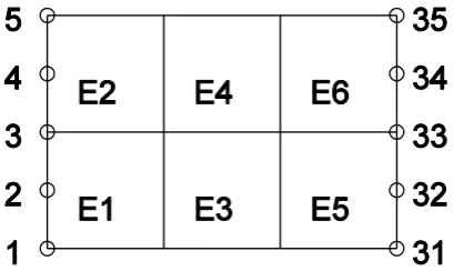
method (Laursen, 2002)). To deliver the idea easily, we selected a simple 2D model mesh as shown in
Fig. 1.
Nodal Collocation Using the nodal collocation, the collocation at all nodes, the boundary integral in Eq. (9) can be written as
5
30 1
0, , , for all .
left k k k k
y L y d k
μ u u μ u u (11)Refer to Fig. 1 for example nodal numbering scheme used in Eq. (11). In this case the block matrix ,
which is a 10 70 matrix, for this specific problem in a symbolic form can be expressed as follows:
I10 10 O10 50 I10 10
, (12)
where the sub-block matrix I10 10 indicates the identity matrix of the size 10 10 and O10 50 is the
null block matrix of the corresponding dimension. Considering the following product of the matrix
10 10 10 50 10 10 10 10 50 10 50 50 50 10
10 10 10 50 10 10
2 and ,
T T
I O I
I O O O
I O I
(13)
we notice that the matrix T is a full-rank matrix, whereas T is not with rank deficiency.
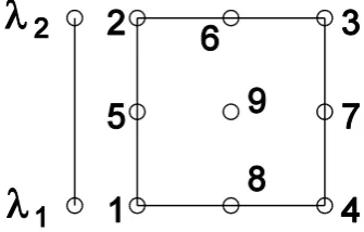
Linear Continuous Interpolation A standard mortar element discretization is much more involved in this case. Introducing the linear interpolation of the Lagrangian multiplier along the 1D element
8
11 2 2
,
N
λ λ
λ
the integral in Eq. (9) along the element boundary can be written as follows:
, 2 , , 10, , .
left e left
T T
e e left e right
e
y L y d N N d u u
μ u u
(14)The symbol
N is the interpolation function for the velocity unknowns and the subscript ' 'eindicates the variable defined within an element. Using the local numbering in Fig. 2, the block matrix
in the specific mesh of Fig. 1 can be expressed in a symbolic form as
3 5 3 5 3 5 3 5 3 5 3 5 3 5 3 5 3 5 3 5
,
U O O U O
O U O O U
(15)
where a sub-block matrix U3 5 is
3 5
1 3 2 3 0 0 0
0 2 3 2 3 2 3 0 .
0 0 0 2 3 1 3
U
Again considering the following two products of the block matrix :
2 2
5 5 5 50 5 5
5 5 5 5
2 2
5 5 5 5 5 50 5 5 5 5
2 3 3
50 5 50 5 50 50 50 5 50 5 2
3 3 2 2
5 5 5 50 5 5
5 5 5 5
2 2
5 5 5 5 5 50 5 5 5 5
2 0 and , 0 2 T T T T T T T T T T
U O O U O
O U O O U
U
O O O O O
U
U O O U O
O U O O U
(16)
the matrix T is found to be a full-rank matrix, whereas T is not with rank deficiency.
2.2. The augmented Stokes flow problem with immersed solid bodies
The second highly constrained Stokes problem of interest in this study is the Stokes flow
with immersed solid bodies. To model this problem, we use the so-called rigid-ring (or rigid-shell in
9
considered as a part of the fluid with the same constitutive equation as the fluid domain with the zero
velocity condition on the solid boundary (Wang and Hwang, 2008; Liu and Hwang, 2009; Liu and
Hwang, 2012). As fluid inertia is neglected in the Stokes flow, the zero velocity condition on the solid
boundary ensures vanishing velocity inside the body. There are three advantages of the rigid-shell
description with the fictitious domain method in simulation of flow in porous media: first, one does
not have to consider the interface conditions between solid and fluid, as the entire problem is
essentially the fluid problem. The second one is the easiness in discretization of the immersed body
using its boundary information only and, as will be shown later, one needs just points on the solid
boundary. Thirdly, as the entire problem is the fluid flow problem, one can use the regular mesh which
facilitates simple implementation for the mortar element technique for the periodic boundary
condition of the representative volume element.
The zero boundary condition on the solid boundary B can be expressed as
0, on B.
u (17)
As was done with the periodic boundary condition, we define the Lagrangian multiplier λ on B
and the zero velocity condition on the boundary can be treated as the constraint in the weak form in
exactly the same form as previous: Find
u, ,p λ
such that
2
: ,t
B
p d D d d d
v
D u v
λ v
t v (18)
0,q d
u (19)0
B d
μ u (20)for all the admissible weighting functions
v, ,q μ
. We employ the point collocation method toimplement the integral over the solid boundary in Eqs. (18) and (20). For example, the integral in Eq.
(20) can be approximated as
1 , M k k B k d
10
where M, xk and μk are the number of collocation points on B, the position of the k-th
colocation point and the collocated Lagrangian multiplier at xk, respectively. The resulting matrix
equation appears exactly the same as the previous periodic boundary condition in Eq. (10). Though
not presented here, the product of the corresponding off-diagonal sub-block matrix satisfies the
same characteristics: the matrix T is a full-rank matrix, whereas T is not with rank deficiency.
3. Block-preconditioning strategy and the generalized eigenvalue problem
For the solution of the matrix equation in Eq. (10), we propose a block preconditioner P
similar to (or motivated by) the Schur complement in the discrete Stokes problem: i.e.,
1 1
0 0
0 0 , with and .
0 0
T T
K
P S S GK G T K
T (22)
The matrix K is a square matrix of the size nunu and is a full rank matrix
rank
K nu
; thematrix G is a non-square matrix of the size npnu is of a full rank
rank
G np
; and thematrix is a non-square matrix of the size nnu is of a full rank
rank
n
. The symbolsu
n , np and n are the numbers of the velocity, pressure and Lagrangian multiplier unknowns,
respectively. The adequateness and performance of the proposed preconditioner can be analyzed by
the eigenvalue problem of the preconditioned system P A1 and therefore the generalized eigenvalue
problem, P Ax1 x with the eigenvalue , can be stated as follows:
0 0
0 0 0 0 .
0 0 0 0
T T
K G u K u
G p S p
T (23)
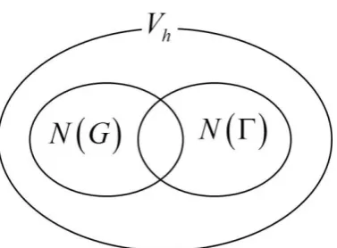
To solve the generalized eigenvalue problem in Eq. (23), we divide the solution space of the
discretized velocity vectors Vh into four subspaces. Now consider the following four subspaces (Fig.
11
◦ Space I: I
h
V N G N ,
◦ Space II: II
c hV N G N ,
◦ Space III: III
c
hV N G N ,
◦ Space IV: IV
c
c hV N G N .
We have some remarks on the four subspaces.
(i) The space N G
is the right null space of the matrix G, which satisfies Gu0 for all
uN G , and the dimension of N G
is
nunp
, since the matrix Gis of full rank.(ii) Similarly, the right null space of the full rank matrix , denoted by N
, satisfies u 0 andhas the dimension of
nu n
.(iii) The dimension of the subspace VhIV is no larger than n or np, which means that
dim N G c N c min n np, .
(iv) The number of unknowns related with the constraint (the periodic boundary condition or the zero
velocity condition) can be safely considered much smaller than the primitive variables u and p,
since the dimension where the constraint is one-order lower than those of u and p: i.e.,
p u
n n n .
The eigenvalue problem in Eq. (23) can be solved exactly for the mutually exclusive four
subspaces. The general procedures involve the block Gaussian elimination process and we summarize
the results below.
Subspace I In this space, Gu0 and u 0. Therefore from Eq. (23) we have a single eigenvalue 1 and the corresponding eigenvector is u 0 0T with u satisfying
0
Gu u . The multiplicity of the eigenvalue is dim
VhI dim
N G
N
.12
0 T
u
with Gu0. By using block Gaussian elimination with Gu0 and 1 T
T K ,
the eigenvalue problem can be reduced to
2
1T 0.
(24)
Since the matrix T is symmetric and positive-definite, we have two distinct eigenvalues
1 2 5 2 whose multiplicity is dim
II hV .
Subspace III In this case, Gu0 and u 0 and the eigenvector can be expressed as 0 T
u p
with u 0. Similarly to the space II, one can obtain the reduced eigenvalue problem
with u 0 and SGK G1 T as follows:
2
1 Sp 0.
(25)
Again, we have two distinct eigenvalues 1 2 5 2 whose multiplicity is dim
III hV , since the
Schur complement matrix S is symmetric and positive-definite.
Subspace IV This is the hardest problem. We notice that uN G
implies urange
GT at least in the eigenvector space of u, since the null space and the row space are mutually orthogonal.In the same way uN
implies urange
T . Further, as the space IV is N G
c N
c, therow space of the two matrices can be identified.
range GT range T , when u V hIV. (26)
The eigenvector in VhIV has the form u p T and u should satisfy uN G
and
uN . By the block Gaussian elimination with Eq. (26), one gets the reduced form of the
eigenvalue problem in VhIV:
2 2
1 1 T 0.
(27)
13
complement matrix T is symmetric and positive-definite.
In summary, the preconditioned matrix P A1 has only six eigenvalues
1, 1 5 2,0,1, 1 5 2, 2
and therefore, once K1, S1 and T1 are computed exactly byany means, the solution of the iterative scheme converges to the exact solution within maximum six
iterations, independent of the problem size. Further, if the solution methods to obtain K1, S1 and
1
T satisfy the O N
performance, the iterative scheme for the entire problem will show theultimate O N
performance.4. Implementation techniques
Although the preconditioner P in Eq. (22) is theoretically optimal, one cannot employ the
preconditioner as is, since the Schur complement SGK G1 T and T K1T involves the
inverse of K which is prohibitively expensive by themselves. Therefore one needs further
approximation of the preconditioning matrix P. In this section, we seek implementation techniques
for the preconditioning problem. As the preconditioners K and S, which are related with the
velocity and the pressure unknowns respectively, are the same as the Stokes flow problem, we can
follow the approach outlined for the Stokes systems (Silvester and Wathen, 1994; Elman et al., 2005;
Hwang et al., 2011a). For the approximation of the preconditioning block matrix , we employ the
discrete Laplace operator ˆK, which can be inverted by an algebraic multigrid (AMG) V-cycle to
provide a fast and efficient solution. Details of analyses on the choice of the discrete Laplace operator
has been presented by the authors’ previous work (Hwang et al., 2011a). The block preconditioner S,
the Schur complement matrix of the Stokes problem, is spectrally equivalent to a mass matrix M in
the pressure space (Elman et al., 2005). Therefore we adopt the mass matrix M in the discrete
pressure space as the approximation of the Schur complement S in the present study and the mass
14
independent of the number of unknowns.
From the above statement, the approximation of the preconditioner, denoted by ˆP, can be
expressed as
ˆ diag ˆ, , .
P K M T (28)
The last remaining problem is the sub-preconditioning problem with T , which can be written as
1
, with T.
Tzr T K (29)
The problem with Eq. (29) is that the block matrix is not a square matrix and its inverse is not
obvious. In this work, we propose an exact solution method for Eq. (29) using the fundamental
solution and present the performance of our scheme in comparison with the approximation method for
the matrix proposed by Elman (1996).
4.1. Implementation of block preconditioning with an approximate solution of the Schur complement
First we start presenting the approximation method for the solution of Eq. (29), which was
originally developed of Elman (1996) and is called as the ‘BFBt’ preconditioner. It is relatively easy
to implement but at the same time the number of iterations for the convergence scales with O
Nand therefore the CPU time scales with O N N
. Here we present a little bit modifiedimplementation scheme to clearly show the procedures, which are composed of three steps as below.
Step 1 [Solution of y r] This can be done by taking y Ty*. Firstly solve for y* *
,
T
y r
(30)
and find y from y Ty*. As illustrated in Eqs. (13) and (16), the matrix T is small and easily
invertible for both the constrained problems. Especially with the nodal collocation, the matrix T
is simply twice of the identity matrix.
15
xAy (31)
Step 3 [Solution of Tz x] This problem can be transformed into a trivial problem by multiplying on both sides, since T is easily invertible.
Tz x
(32)
The whole solution process requires two matrix inversions in the form of Tx b and
three matrix-vector multiplications among which one is hugh xAy and the other two are small.
Though it looks concise and clear, the final solution of Eq. (32) is not exact but only an approximation.
The reason is that x in Eq. (32) does not reside in the range of T in general and the equation in
the third step Tz x does not have exact solution. Therefore, one may expect minor improvement
in iterative performance and as will be seen later the number of iterations scales with O
N .4.2. Implementation of block preconditioning with the fundamental solutions
In the present work, we propose an exact solution of Eq. (29) using the fundamental
solutions and with this method we start rewriting Eq. (29) as follows: Find z satisfying
,
Tz Ky
(33)
subjected to the constraint of
.
y r
(34)
In this method, we represent the solution z in terms of y which resides in the column space of
1 T
K , or range
K1T
. Let i be the i-th column vector of T, which is an nun matrix.1 2
| | |
.
| | |
T
n
(35)
We notice that n nu in the constrained problems of this study, since the Lagrangian multiplier is
16
the i vectors are independent each other as the matrix T is of a full rank. That is, rank
T n.Now one can express the right-hand side of Eq. (33) as a linear combination of the i vectors with
the constant coefficient zi’s:
1 . n T i i i z z
(36)Let y*i be the fundamental solution of the problem.
*
, 1, ,
i i
Ky i n (37)
The name ‘fundamental solution’ seems to be proper for two reasons: one is that *
i
y is the solution
for each column vector of T and the other is that the solution of Eq. (34) can be represented as a
linear combination of *
i
y such that
* 1 . n i i i
y z y
(38)Finally one can get the exact solution of Eq. (34) subjected to the constraint of Eq. (35) by solving the
linear system below:
* * *
1 2
| | |
, with and .
| | |
n
Tz r T Y Y y y y
(39)
The matrix T is the exactly Schur complement defined in Eq. (22) and is an nn square matrix
whose component is a simply inner product of i and *
i
y :
*
, , 1, , .
ij i j
T y i j n (40)
From Eq. (40) one identifies that the matrix T is unsymmetric and almost full matrix. We have
several remarks on this method.
(i) This scheme is based on the fact that the number of Lagrangian multipliers is much smaller that
that of the velocity unknowns, which is valid in the periodic boundary condition and the immersed
17
(ii) The most time-consuming step is Eq. (37) for the solution of the complete fundamental solution
set *
i
y ’s. However one can construct the AMG matrix only once and use it repeatedly for all right
hand side vectors i’s with the splitted AMG method. This facilitates significant saving in
computation time and moreover the AMG method has the O N
performance. (The memoryusage and CPU time scales linearly with the number of unknowns.)
(iii) For the problems of interest in this work, the matrix does not change even in the time
dependent problem or problems with nonlinear material properties (e.g. shear-thinning viscosity)
and this means that one can construct the Schur complement T once and use it for all.
(iv) As every fundamental solution *
i
y is independent, it is not necessary to build the matrix Y
explicitly, which is a hugh matrix. In practice, one can introduce a temporary vector as a
fundamental solution and use it to build the j-th column of the matrix T by using Eq. (40).
(v) As the Schur complement matrix T is completely full, there is no advantage to use a sparse
matrix storage and related solution technique in solving Eq. (39). We use a simple LU
decomposition provided in LINPACK. The LU decomposition can be used for all repeated, which
invokes significant reduction in computation time as well. Therefore, this method does not require
any additional storage other than the matrix T itself.
5. Numerical examples
The first test problem is a 3D cubic channel Stokes flow of the size 1 1 1 with the
pressure drop in one direction, where the periodic boundary condition is applied. We tested the two
interpolation schemes for the Lagrangian multipliers, the nodal collocation and the linear continuous
interpolation. Three different finite element meshes have been employed from coarse to fine: 5 5 5 ,
10 10 10 and 20 20 20 . Note that the number of unknowns increases by the factor of 64. In all
the computational results presented here, the number of V-cycles in the AMG is set to six and the
18
the original right-hand side vector b, i.e. r b 107 as the convergence criteria.
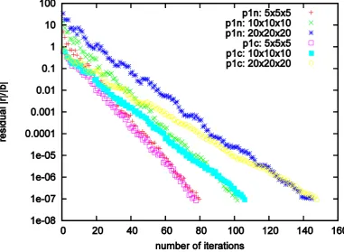
Plotted in Fig. 4 are the convergence behaviors of the iterative scheme based on the
approximation of the Schur complement discussed in Sec. 4.1. In both the results, the number of
iteration for the convergence is found to increase with the number of unknowns and more specifically
results show that the number of iterations indeed scales with O
N , which is consistent to theresult presented by Elman (1996).
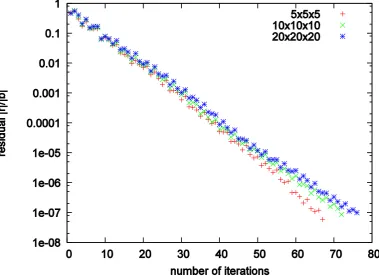
Having validated the correctness of our code, we tested the proposed exact Schur
complement method using the fundamental solution and the results are presented in Fig. 5. Plotted in
Fig. 5 are the convergence behaviors for the same 3D Stokes problem in a cubic channel with the
periodic boundary condition implemented with the exact Schur complement scheme using the
fundamental solution for the linear continuous interpolation of the Lagrangian multipliers. Fig. 5
shows monotonic exponential convergence (nearly straight line) and that the number of iterations of
the outer MINRES algorithm to reach convergence is roughly constant irrespective of the problem
size. As was already shown in Hwang et al. (2011a) and Eq. (28), the AMG algorithm for the
preconditioning velocity unknowns
Kzˆ r
has O N
expenses in both memory and CPU timeand the preconditioning for the pressure variable
Mzr
with the diagonally scaled CG convergeswithin a single iteration for this specific choice of the pressure discretization, the overall performance
can be expected to be close to O N
in both the memory usage and computation time. It is close tothe ultimate O N
convergence, since there is one exception in the proposed iterative scheme. Theonly exception is the solution of the preconditioning problem in (39) involving the LU decomposition
and related full matrix construction. (A hugh problem with Eq. (37) involves the inverse of the
matrixKbut we employ the AMG as mentioned in Sec. 4.2 which has the O N
performance byitself.) However, since the Lagrangian multiplier is defined in the space one order lower than those of
19
Lagrangian multiplier variables can be expected minor. In summary, the iterative solution technique
with the fundamental solution for the exact Schur complement shows nearly the O N
convergence,because the outer MINRES iteration converges within the fixed number of iteration and, among the
three block preconditioning schemes, two large problems related to the velocity and pressure
unknowns has the O N
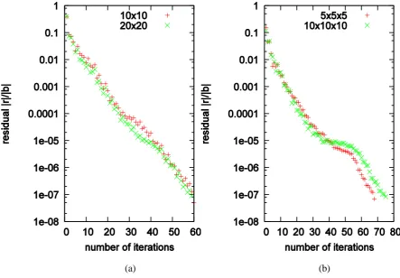
convergence.Finally we present the convergence behavior of the Stokes flow problem with an immersed
solid body in Fig. 6. A circle of radius 0.15 is centered in a domain of the size 1 1 in the 2D
problem and a sphere of radius 0.15 is centered in a domain of the size 1 1 1 as for the 3D problem.
The particle boundary is discretized with uniformly distributed (collocation) points and non-trivial
task in obtaining uniformly spaced points on a spherical surface has been performed by using the
spiral point-set method (Saff and Kuijlaars, 1997). The numbers of collocation points were 21 with a
20 20 mesh in 2D and 81 with a 10 10 10 mesh in 3D and they were chosen to scale with the
number of elements for larger or smaller problems. The same pressure difference boundary condition
as previous is applied such that the circle (or sphere) is an obstacle for flow separation. In 2D problem
(Fig. 6a), one can again observe monotonic exponential convergence along with the fixed number of
iteration for both 10 10 and 20 20 meshes indicating mesh-independent number of outer
iterations, as in the previous periodic boundary problems. However, we observed convergence stalling,
around the residual value of 105, though global convergence behavior is somewhat satisfactory. We
need further investigation for the origin of the convergence stalling. From our previous experience on
the Stokes flow, this phenomenon might be related with modification of the singularity behavior by
introducing the (non-singular) preconditioner (Hwang et al. 2011a), where the pressure specification
to remove singularity in all Dirichlet boundary conditions invokes adverse effects such as
convergence stalling (delay in the convergence rate) counter to common wisdom. Similarly, Elman et
al. (2005) reported that rank deficiency for an enclosed flow does not prevent convergence to a
20
in direct solver might yield additional constraints to the matrix system to be an over-constrained
problem.
6. Conclusions
In this work, we have presented a new efficient iterative scheme to apply large-scale 3D simulations
of flows in porous media, using on the optimal block-preconditioning and the combination of the
Krylov-subspace/AMG method and the exact Schur complement method with the fundamental
solution. The use of the exact Schur complement can be justified by the fact that the Lagrangian
multipliers are defined in the space one order lower than those of the primitive variables, which is
particularly true for the periodic boundary constraint and the zero velocity condition on the immersed
solid body boundary which are the two main ingredients for successful flows simulations in porous
media with the representative volume element (unit cell). The block preconditioner has been proposed
by solving the generalized eigenvalue problem to result in only six different eigenvalues of the
preconditioned matrix system. Further, we proposed the exact Schur complement method using the
fundamental solution. We illustrated the performance of the present solver through example problems
in 2D and 3D, in comparison with the approximate Schur complement method. We reported that the
number of iterations to reach the convergence is independent of the problem size, which implies that
the performance of the present iterative solver is close to O N
.Further development of the iterative solution techniques of this class is necessary particularly
for flow simulations with complex fluids such as viscoelastic fluids, particle suspensions, droplet
emulsions and/or fiber suspensions, in which one always wants to solve large-scale 3D flow problems
to understand hydrodynamic interactions, particle-particle/droplet-droplet interactions in various
ranges. The next step would be the development of a similar iterative solution method for massive 3D
simulations of particle or fiber suspensions (e.g., Hwang et al., 2011a). The periodic boundary
conditions and the treatment of immersed solid body in this work can be extended to solve particle
21
Acknowledgement
This work was supported by the National Research Foundation of Korea (NRF) funded by the
Ministry of Education, Science and Technology (2011-0031383 and 2010-0021614).
References
Elman, H.C., 1996, Preconditioning for the steady-state Navier-Stokes eqautions with low viscosity,
SIAM J. Sci. Comput., 20, 1299-1316.
Elman, H.C., D.J. Silvester, A.J. Wathen, 2005, Finite Elements and Fast Iterative Solvers with
Applications in Incompressible Fluid Dynamics, Oxford University Press, New York.
Hwang, W.R., S.G. Advani, 2010, Numerical simulations of Stokes-Brinkman equations for
permeability prediction of dual-scale fibrous porous media, Physics of Fluids, 22, 113101. Hwang, W.R., M.A. Walkley, O.G. Harlen, 2011a, A fast and efficient iterative scheme for viscoelastic
flow simulations with the DEVSS finite element method, J. Non-Newtonian Fluid Mech., 166, 354-362.
Hwang, W.R., W.R. Kim, E.S. Lee and J.H. Park, 2011, Direct simulations of orientational dispersion
of platelet particles in a viscoelastic fluid subjected to a partial drag flow for effective coloring of
polymers," Korea-Australia Rheol. J. 23, 173-181.
Laursen, T.A., 2002, Computational Contact and Impact Mechanics, Springer, Berlin.
Saff E.B., and A.B.J. Kuijlaars, 1997, Distributing many points on a sphere, Mathematical
Intelligencer, 19, 5-11.
Silvester, D.J. and A. J. Wathen, 1994, Fast iterative solution of stabilized Stokes systems. Part II:
Using general block preconditioner, SIAM J. Numer. Anal., 31, 1352-1367. Strang, G., 2007, Computational Science and Engineering, Wellesley, Cambridge.
Wang, J.F., and W.R. Hwang, 2008, Permeability prediction of fibrous porous media in a bi-periodic
22
Liu, H.L., and W.R. Hwang, 2009, Transient filling simulations in unidirectional fibrous porous media,
Korea-Australia Rheol. J., 21, 71-79.
Liu, H.L., and W.R. Hwang, 2012, Permeability prediction of fibrous porous media with complex 3D
23
List of Figure Captions
Figure 1: A 2D model mesh (left) and local node numbering in an element (right).
Figure 2: An example 1-D element for the linear interpolation of the Lagrangian multipliers.
Figure 3: Subspaces of the solution space Vh of the velocity unknowns.
Figure 4: Convergence behaviors of the iterative technique for 3D Stokes problem with the periodic
boundary condition implemented with the approximate Schur complement scheme for both
nodal collocation and linear continuous interpolation of the Lagrangian multipliers. ‘p1n’
indicates results from the nodal collocation and ‘p1c’ is for the linear continuous interpolation.
Figure 5: Convergence behaviors of the iterative technique for 3D Stokes flow with the periodic
boundary condition implemented with the exact Schur complement scheme using the
fundamental solution for the linear continuous interpolation of the Lagrangian multipliers.
Figure 6: Convergence behaviors for 2D (a) and 3D (b) Stokes flow with an immersed solid body
24
25
26
27
28
29
Figure 6: Hwang et al.