Concentric Symmetry

White Rose Research Online URL for this paper:

http://eprints.whiterose.ac.uk/79880/

Version: Submitted Version

Monograph:

Silva, F.~N., Comin, C.~H., Peron, T.~K.~D. et al. (5 more authors) (2014) Concentric

Symmetry. Working Paper.

[email protected] https://eprints.whiterose.ac.uk/

Reuse

Items deposited in White Rose Research Online are protected by copyright, with all rights reserved unless indicated otherwise. They may be downloaded and/or printed for private study, or other acts as permitted by national copyright laws. The publisher or other rights holders may allow further reproduction and re-use of the full text version. This is indicated by the licence information on the White Rose Research Online record for the item.

Takedown

If you consider content in White Rose Research Online to be in breach of UK law, please notify us by

Filipi N. Silva1_{, Cesar H. Comin}1_,∗

Thomas K. DM. Peron1_{, Francisco A. Rodrigues}2_,

Cheng Ye3_{, Richard C. Wilson}3_{, Edwin Hancock}3_{, and Luciano da F. Costa}1

1_{Instituto de Física de São Carlos, Universidade de São Paulo, São Carlos, São Paulo, Brazil} 2_{Departamento de Matemática Aplicada e Estatística,}

Instituto de Ciências Matemáticas e de Computação,Universidade de São Paulo, Caixa Postal 668,13560-970 São Carlos, São Paulo, Brazil

3_{Department of Computer Science, University of York, York, YO10 5GH, United Kingdom}

The quantification of symmetries in complex networks is typically done globally in terms of au-tomorphisms. In this work we focus on local symmetries around nodes, which we call connectivity patterns. We develop two topological transformations that allow a concise characterization of the different types of symmetry appearing on networks and apply these concepts to six network models, namely the Erdős-Rényi, Barabási-Albert, random geometric graph, Waxman, Voronoi and rewired Voronoi models. Real-world networks, namely the scientific areas of Wikipedia, the world-wide airport network and the street networks of Oldenburg and San Joaquin, are also analyzed in terms of the proposed symmetry measurements. Several interesting results, including the high symmetry exhibited by the Erdős-Rényi model, are observed and discussed.

I. INTRODUCTION

The study of graph symmetry has its roots in algebraic graph theory [1–4]. In this context, symmetry is defined in terms ofautomorphismsand theorbits of the nodes in a given graph. More specifically, an automorphism of a graphGis a permutation of the vertex labels which pre-serves the label adjacency relation of the original graph. The orbit of a given vertex is the set of remaining vertices that share a label over the permutations in a automor-phism group [1–4]. It is then assumed that a network is symmetric if it has at least one vertex label permutation such that the label adjacency remains unchanged. Oth-erwise, the network is considered to be asymmetric [1–5]. Despite the great amount of work devoted to the struc-tural and dynamical characterization of complex net-works, the study of symmetry has received less attention, including works such as [5–7]. In algebraic graph the-ory, the study of symmetry is focused on simple graphs. More recently, measurements based on automorphisms and orbits have been employed to analyse the structure of complex networks. For instance, Xiao et al. [5] ap-plied the size of automorphisms groups [7] to quantify the symmetry of real-world complex networks, showing that the emergence of symmetry in such networks is a conse-quence of similar patterns of connectivity. Furthermore, in [5] the authors proposed a variation of the preferential-attachment mechanism in which new nodes are connected with probability proportional to the degree of previously existing nodes together with their local symmetry. Inter-estingly, the model was capable of reproducing the sym-metry properties observed in real-world networks, rein-forcing the hypothesis that similar linkage properties are crucial for the emergence of overall symmetry [5].

While symmetry measurements based on

automor-∗_{Electronic address: [email protected]}

phisms typically apply to the whole graph, it is also pos-sible to develop approaches aimed at quantifying sym-metry locally, for instance using a given reference node. One of the first studies of local symmetry in complex networks was reported by Holme [6], where the so-called degree-symmetryof a node was proposed. Although this allowed the local symmetry to be quantified with respect to a reference node, occasional negative values can be obtained. Also, that measurement does not posses clear bounds, making the comparison of the symmetry of pat-terns with different structures less clear.

There are several reasons why to quantity the topo-logical symmetry around specific nodes of a network. To begin with, the intrinsic way in which several networks, synthetic or real, are constructed, tends to imply a char-acteristic local symmetry. For instance, patterns in city networks should reflect the grid-like organization typi-cally adopted in urban planning. On the other hand, the hubs in scale free networks could be expected to disrupt the local symmetry. Interestingly, such types of sym-metries characteristic to different networks are also ex-pected to impact the dynamics unfolding in the respec-tive structure. For instance, highly symmetric patterns would be expect to promote a more uniform traffic flow in a city. Though the previously introduced [8] accessi-bility measurement has been found to provide valuable information about the local properties of the topology around a node (e.g. it can be used to define the borders of a network [9], it is highly influenced by its degree, and therefore becomes related to many other degree-related measurements. Contrariwise, the value of the local sym-metry should not be directly influenced by the degree of the reference node, which can be done by a suitable normalization.

Here, as in [6], we study local symmetry across the concentric levels of a reference node, where a concen-tric level is defined as the set of nodes having the same shortest path length to the reference node. However, our definition of symmetry is based on the accessibility of a

node [8, 10], which is also a concentric measurement. The accessibility of a node for a given concentric level is calcu-lated from the transition probabilities of that node to the neighbors at that level. These transition probabilities are defined by the dynamics imposed on the network, such as self avoiding random walks or epidemic spreading. The accessibility of a node is high when the transition proba-bilities at that given concentric level tend to be uniform. The number of nodes in a concentric level is referred to as the number of reachable nodes. The accessibility of the concentric level attains its maximum value when all tran-sition probabilities at that level are equal. In this case, the accessibility, or effective degree, of the reference node becomes equal to the number of reachable nodes, indi-cating that they can be optimally accessed. We combine a normalized version of accessibility with a variation of the random walk dynamics, referred to as the concentric random walk, to evaluate the symmetry of the concen-tric level of nodes in the network. This specific type of random walk is adopted in order to avoid transitions of moving agents to previous concentric levels, which would otherwise reduce the exploration of the remainder of the network. Two symmetry indices can be derived from this type of dynamics. The first is thebackbone symmetry, in which the links inside a concentric level are eliminated (no transition between them). The second is themerged symmetry, in which these links assume cost zero in the transition. As such, these two indices provide comple-mentary quantification of the local symmetry around a given node.

Complex networks have been defined as graphs with a topology that is moreirregular than that in a uniformly random model such as Erdős-Rényi [11]. Formally, a graph is said to be regular[3] if all its nodes have the same degree, implying some level of uniformity and sim-plicity. However, it is known that the degree alone is not sufficient to completely specify a graph. So, thecomplex in complex networks actually refers to intricate distribu-tions not only of degree, but also of other measurements, as discussed in [11]. In this context, the two measure-ments proposed in the current article can be understood not only as a quantification of node-centered symmetry, but also as a more robust evaluation of its regularity, and thereforesimplicity, of the network. In other words, com-plex networks could be characterized and even defined as graphs possessing several nodes presenting high values of backbone and merged symmetry measurements.

This paper is organized as follows: Section II presents our modification of the accessibility measurement, which are used to define the backbone and merged symmetry measurements. Section III is devoted to the characteriza-tion of symmetry patterns emerging in random network models. The same analysis is performed for real-world networks in Section V. Finally, conclusions are presented in Section VI.

II. THE BACKBONE AND MERGED

SYMMETRIES

The two symmetry measurements are defined here for each concentric level [12]Γ(ih)of a given reference nodei,

where the concentric level is defined as the set of nodes that are at topological distancehfrom i. For example, the first concentric level is the set Γ(1)i of neighbors of

node i. The symmetries are calculated in terms of the transition probabilities of aconcentric random walk. In this type of dynamics, the agent cannot return to the pre-vious concentric level, which would be detrimental to the diffusion to more distant levels. For the same reason, i.e. to enhance the exploration of further levels, the edges be-tween nodes belonging to a same concentric level should be treated differently. There are two ways to deal with these intra-level edges: (i) to remove then; and (ii) to join the nodes which they interconnect. This gives rise to two intermediate representations of the pattern. Therefore, the concentric random walk is specified with respect to these two structures, as explained in this section.

In the remainder of this work, we will always use the terms backbone and merged to refer, respectively, to the infinite-cost and zero-cost transitions over edges within concentric levels.

The backbone and merged representations can provide complementary information about the topological sym-metry of the neighborhood of a node, therefore we define a symmetry measurement for each representation, which we call backbone symmetry and merged symmetry, re-spectively. Both symmetries are obtained by treating the backbone and merged patterns as follows. We represent as P(h)_{(i→j)the probability that a walker undergoing}

a concentric random walk goes from nodeito node j in

hsteps. This allow us to define the following transition probabilities for nodesj belonging to the setΓ(ih)

P(h)_{(i→j|i→k,∀k∈Γ}(h)

i ) =

P(h)_(i→j)

P

k∈Γ(h)

i

P(h)_(i→k), (1)

This expression can be understood as the probability of the walker being at nodej, given that it arrived at some node of theh-th concentric level of nodei. For simplic-ity’s sake, we henceforth replaceP(h)_{(i→j|i→k,∀k∈}

Γ(ih)) by P(h)(i → j|i → Γ (h)

i ). We then calculate the

Shannon entropy of the transition probabilities as

H_i(h)=− X

j∈Γ(ih)

P(h)(i→j|i→Γ(_ih)) ln[P(h)_(i→

j|i→Γ(_ih))]

=− X

j∈Γ(ih)

P(h)_(i→j) P(h)_(i→Γ(h)

i )

ln P

(h)_(i→j) P(h)_(i→Γ(h)

i )

!

. (2)

Now defining ξi(h) as the set of reachable nodes from

nodei, for walks of lengthh(i.e.,ξ(ih)={j|P(h)(i→j)>

0}), we calculate the respective symmetry measurement as

Si(h)=

eHi(h)

|ξ(ih)|

(3)

where |X| is the cardinality of the set X. Therefore, to each node of the network the backbone and merged sym-metry measurements,{Sb(ih), Sm

(h)

i }, are assigned to the h-th concentric level of node i. We use the exponential of the entropy in order to have the number of reachable nodes as dimension [8], which is more intuitive and com-patible with|ξi(h)|. Observe that both measurements of

symmetry are bounded between 0 and 1.

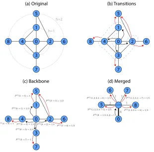
These measurements are illustrated in the following example. For the 2-pattern shown in Figure 2(a), we cal-culate the two symmetry measurements for node 0 with respect to the second concentric level. First, we create the backbone and merged patterns, as shown in Figures

2(b) and (c). The backbone pattern is the original net-work without the connections within the first concentric level. For the merged pattern, nodes 1,2,3 and 4 are merged into a single node, and this new node connects to all neighbors of the merged nodes. Since four con-nections between concentric levels were merged into a single one, the new connection between node 0 and the merged node has weight 4. For the backbone pattern, Γ(2)₀ ={5,6,7,8} and ξ₀(2) ={5,6,7,8}. Therefore, the entropy of the transition probabilities is calculated as

H₀(2)=− X

j∈Γ(2)₀

P(2)_(0→j)

P(2)_(0→Γ(2)

0 )

ln P

(2)_(0→j)

P(2)_(0→Γ(2)

0 )

!

=−41/4 1 ln

_1/4

1

= ln(4)

The backbone symmetry is then given by

Sb(2)0 =

eH₀(2)

|ξ0(2)|

= 4 4 = 1.

For the merged pattern, the calculation is analogous, but with the difference that the edge weights are incorpo-rated into the transition probabilities. In this case, both measurements attain the maximum possible value, which is expected since the original pattern is symmetric.

In Figure 2(d) we provide another example where the neighborhood of the node is not perfectly symmetric. The respective backbone and merged patterns are shown in Figures 2(e) and (f). Note that a self-loop is added to node 3 of the backbone pattern. This is done because when the walker reaches node 3 it becomes trapped at that node. The probability of being at node 3 is not considered when calculatingH0(2), since only the

transi-tion probabilities to nodes at the second concentric level are relevant. Nevertheless, the self-loop is still neces-sary because node 3 is in the set of nodes reachable from node 0. Therefore, the nodes in the second con-centric level areΓ(2)₀ ={5,6,7} and the reachable nodes are ξ₀(2) ={3,5,6,7}. The remaining calculation is the same as above. For this case, the backbone symmetry is

Sb(2)0 = 0.75and the merged symmetry isSm (2)

0 = 0.97.

III. NETWORK MODELS

Let us start by characterizing the Erdős-Rényi (ER) model in terms of the backbone and merged symmetries

{Sb(_ih), Sm(_ih)}. In Figure 3 we show the scatterplots of

Sb(ih) as a function of Sm (h)

i for h= 2 and 3, together

0 4

8 2 6

3 7 5 1 0 4

8 2 6

3

7 5

1 (b) Transitions

(c) Backbone (d) Merged

0 5 1,2,3,4

4 4

/ 1) = 1 → (0 (1) P 4 / 2) = 1 → (0 (1) P 4 / 3) = 1 → (0 (1) P 4 / 4) = 1 → (0 (1) P

5) = 1 → (1 (1) P

7) = 1 → (3 (1) P 8) = 1 → (4 (1) P 2 1 1 1

4) = 1 , 3 , 2 , 1 → (0 (1) P 6 7 8 0 4

8 2 6

3 7 5 1 (a) Original 2 / 6) = 1 → (2 (1) P 2 / 5) = 1 → (2 (1) P 5 / 5) = 2 → 4 , 3 , 2 , (1 (1) P 5 / 6) = 1 → 4 , 3 , 2 , (1 (1)

P _P(1)(1,2,3,4→7) = 1/5

5 / 8) = 1 → 4 , 3 , 2 , (1 (1) P h=1 h=2

FIG. 1: Illustration of the concentric random walk dynamics. (a) Original 2-pattern considered, with concentric levels indicated by dashed lines. (b) One step transitions allowed for the random walk, indicated by arrows. Black and red arrows are for transitions departing from, respectively, the first and second concentric levels. Nodes inside the blue dashed line form a connected group inside the first concentric level. Treating the connections between these nodes as infinite-cost or zero-cost is equivalent to representing the original pattern as, respectively, the (c) backbone and (d) merged patterns.

0 0

5,6

1,3,4

7 2

7 4 2 6

3 1 5

(d) Original (e) Backbone (f ) Merged

4 / 7) = 1 → (0 (2)

P _P(2)(0→6) = 1/4

4 / 3) = 1 → (0 (2) P 4 / 5) = 1 → (0 (2) P

(a) Original (b) Backbone (c) Merged

0 4

8 2 6

3 7 5 1 0 4

7 2 6

3 5

1

0 4

8 2 6

3 7 5 1 0 8 6 7 5 1,2,3,4 4 / 5) = 1 → (0 (2) P 4 / 6) = 1 → (0 (2) P 4 / 7) = 1 → (0 (2) P 4 / 8) = 1 → (0 (2) P 4 / 5) = 1 → (0 (2) P 4 / 6) = 1 → (0 (2)

P _P(2)(0→7) = 1/4

4 / 8) = 1 → (0 (2) P 4 1 1 1 1 3 1 1 1 1 8 / 7) = 3 → (0 (2) P 8 / 6) = 5 , 5 → (0 (2) P

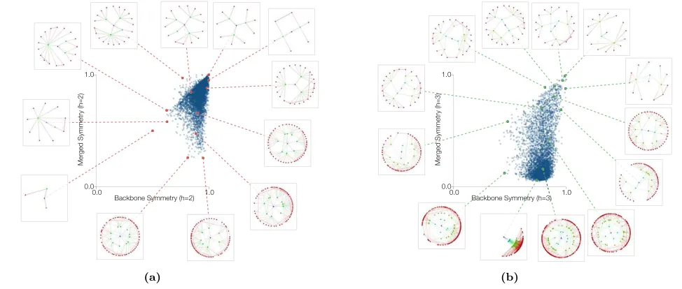
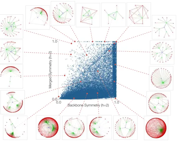
density of subgraphs occurring for values of Sb(2)i close

toSm(2)i , with a great homogeneity of observed patterns.

Note, also, that most of these patterns are tree-like, i.e., without the presence of triangles. This pattern is fre-quently found in uncorrelated networks [13]. Therefore, for low values ofh, the ER model yields highly symmetric patterns, essentially as a consequence of the aforemen-tioned tree-like characteristic of the network.

The scenario changes as we increase the value of h. For h = 3 (Figure 3 (b)), the symmetry values are smaller than in the former case. This effect is stronger for the merged symmetry. This can be explained by the small-world characteristic of the ER model. Since these networks have average shortest path lengths of or-derℓ ∼lnN, with a few steps all nodes can be reached (given that the networks contains only one connected component), becoming highly unlikely that a symmetric structure is obtained. Any eventual connection between the same level will not change the backbone symmetry, but will strongly impact on the merged symmetry. Since for largerhthe probability of having a connection on the same level is larger, the merged symmetry values tend to decrease. Note in Figure 3 that patterns below the line

Sm(2)=S_b(2)often present a higher number of connections

(see Figure 14).

Next we turn our analysis to spatial random graphs in order to study spatial effects on the symmetry of pat-terns. First we consider the random geometric graphs (GEO) whose nodes are connected if they are separated by distances smaller than a certain distance [14]. As we can see in Figure 4, the GEO network behaves similarly to the ER model, though with more accentuated decrease in the merged symmetry as we increase the value of h. Unlike the ER model, GEO networks do not have local tree-like structures, but rather a high number of triangles implied by connecting all nodes within a certain radius. The increase in the clustering coefficient leads, therefore, to more connections between nodes at the same concen-tric level, a fact that is reflected by the larger dispersion in the values of the merged symmetry for h= 2in Fig-ure 4(a). Moreover, forh= 3(Figure 4(b)), we observe a striking difference between the GEO networks and the ER structures. Although perfectly symmetric patterns can still be observed, the symmetry of the merged pat-terns decrease significantly, suffering even more the ef-fects of high clustering.

Another example of a spatial random graph, namely the Waxman model (WAX) [15, 16], is shown in Figure 5. Interestingly, both symmetries tend to be smaller than the values obtained for GEO. It is worth noting that there is a non-vanishing probability of observing long-distance connections in the WAX model, a fact that might explain the loss of backbone symmetry for larger values ofh.

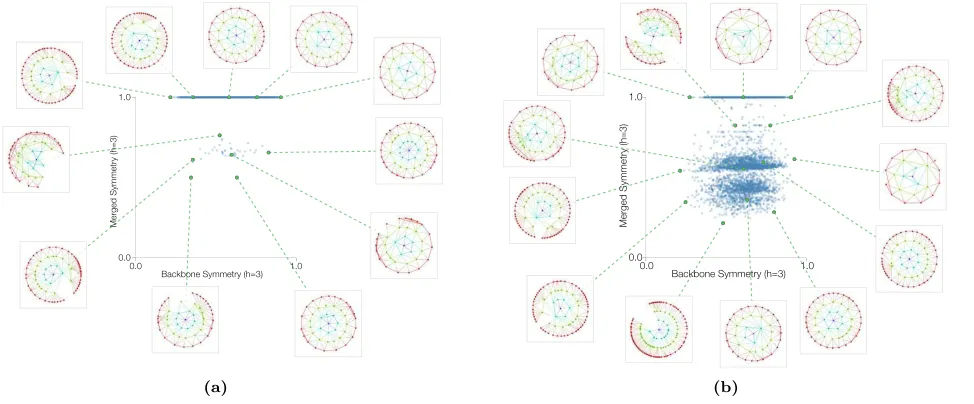
Voronoi networks [16–18] (VOR) are typically obtained from a given spatial distribution of nodes in a metric space, and pairs of nodes are interconnected whenever their Voronoi cells touch one another. Figure 6(a) illus-trates the backbone and merged symmetries for h = 3,

as well as some representative patterns. Figure 6(b) presents analogue results obtained for a rewired Voronoi network (RVOR), obtained by randomly selecting links in the previous network and placing them between a ran-domly chosen pair of nodes (the rewiring probability is

0.001).

The Barabási-Albert (BA) model is our final example considering network models. We note in Figure 7 that the most symmetric patterns are those centered at nodes with smaller degree. On the other hand, hubs have lower values of merged symmetry, as high degrees tend to imply larger probability of reaching non-symmetric regions in the network.

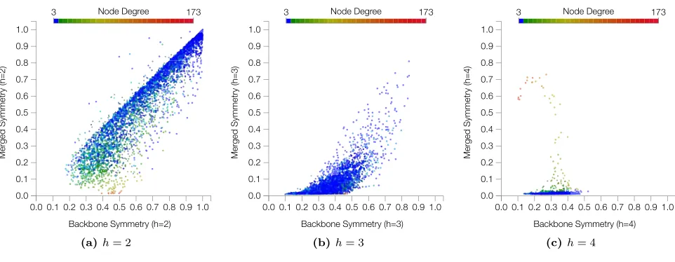
It is also interesting to verify how the symmetry values correlate with the node degrees. We include in Appendix A scatterplots of the backbone and merged symmetries for the second, third and fourth concentric levels. We colored the symbols according to the degree of the ref-erence node. For all models (shown in Figures 14, 15, 16, 17, 18 and 19), except BA, nodes with higher de-grees tend to present lower symmetry values, specially for the merged symmetry. This happens because nodes with larger degrees commonly have more nodes at their initial concentric levels. Since it is less probable that pat-terns having a large number of nodes remains symmetric, such nodes have lower level of symmetry.

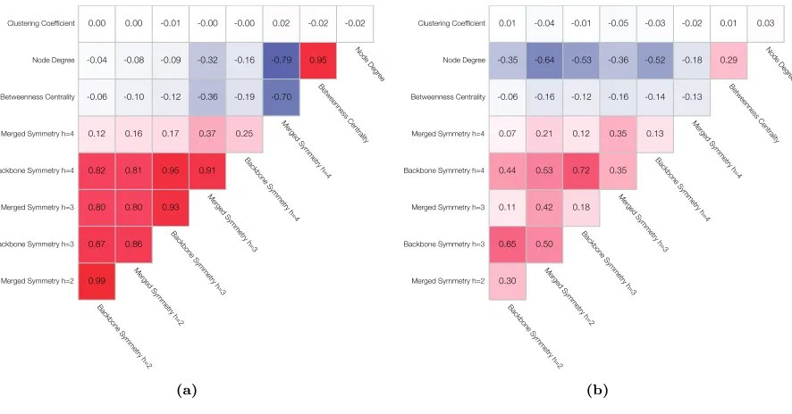
We also investigate the correlations between the sym-metry measurements and between these and three tradi-tional topology measurements, namely the degree, clus-tering and betweenness centrality. The Pearson correla-tion values, organized as a matrix, obtained for the ER and WAX networks are shown in Figures 8(a) and (b), respectively. The results are given only for two models because the correlation matrix of the BA case are sim-ilar to those of the ER model, and the matrix of the GEO network are similar to the WAX case. The back-bone symmetry forh= 2,3,4 and merged symmetry for

h= 2,3 show strong correlations among themselves for the ER model. This is a consequence of the high regular-ity of this model, where the same neighborhood patterns appear at different concentric levels. The WAX model shows less correlation between the symmetry measure-ments, which might be caused by the large variability of patterns characteristic of this model. Also, there is low correlation between the symmetry measurements and the traditional ones, which indicates that the new measure-ments defined in the current work provide complemen-tary information about the network structure that is not contained in the traditional ones.

IV. REAL-WORLD NETWORKS

We also illustrate the potential of the proposed symme-tries for characterizing the local structure of some real-world networks.

0.0 1.0 Backbone Symmetry (h=2) 0.0

1.0

Merged Symmetry (h=2)

Backbone Symmetry (h=2)

Merged Symmetry (h=2)

(a)

0.0 1.0

Backbone Symmetry (h=3) 0.0

1.0

Merged Symmetry (h=3)

Backbone Symmetry (h=3)

Merged Symmetry (h=3)Merged Symmetry (h=3)

(b)

FIG. 3: Symmetries of the ER model for (a)h= 2and (b)h= 3. The network hasN= 5×103_{and average degreehki= 6.}

0.0 1.0

Backbone Symmetry (h=2) 0.0

1.0

Merged Symmetry (h=2)

1.0 Backbone Symmetry (h=2) Backbone Symmetry (h=2)

Merged Symmetry (h=2)Merged Symmetry (h=2)

(a)

0.0 1.0

Backbone Symmetry (h=3) 0.0

1.0

Merged Symmetry (h=3)

Backbone Symmetry (h=3) Backbone Symmetry (h=3) Backbone Symmetry (h=3) Backbone Symmetry (h=3) Backbone Symmetry (h=3) Backbone Symmetry (h=3)

Merged Symmetry (h=3)Merged Symmetry (h=3)Merged Symmetry (h=3)

(b)

FIG. 4: Symmetries of the GEO model for (a)h= 2and (b)h= 3. The network hasN= 5×103 _{and average degreehki= 6.}

pairs of airports are connected if they share a route [26]. Interestingly, a whole different scenario is observed than those obtained for the random graphs examples. For in-stance, we see that the pairs of{Sb(ih), Sm

(h)

i } are much

more distributed in the airport network than in all mod-els. Analyzing the patterns in Figure 9, one interesting behavior is that a significant number of patterns have maximum values for one of the symmetries. For those with S_b(2) = 1, it is possible to observe that they corre-spond to patterns centered at nodes with low degrees con-nected to hubs, yielding tree-like patterns. These nodes represent small airports connected to larger airports that

naturally have many connections. The patterns lying at

S2

m= 1correspond to highly clustered patterns, mainly

composed by links at the same concentric level.

A similar behavior is shown in our next example, for the scientific areas of the Wikipedia network (N = 45876

and hki ≈ 5.8). Here we consider that two pages in Wikipedia are connected if one is cited by the other, ig-noring the direction of the citation. Again, as we can see in Figure 10, the dispersion in the symmetry space contrasts to the model cases as well as the previously observed patterns.

0.0 1.0 Backbone Symmetry (h=2) 0.0

1.0

Merged Symmetry (h=2)

Merged Symmetry (h=2)Merged Symmetry (h=2)Merged Symmetry (h=2)Merged Symmetry (h=2)

Backbone Symmetry (h=2) Backbone Symmetry (h=2)

FIG. 5: Symmetries for a WAX network withN= 5×103 _{andhki= 6.}

0.0 1.0

Backbone Symmetry (h=3) 0.0

1.0

Merged Symmetry (h=3)

Merged Symmetry (h=3)Merged Symmetry (h=3)Merged Symmetry (h=3)Merged Symmetry (h=3)

1.0 1.0 Backbone Symmetry (h=3) Backbone Symmetry (h=3)

(a)

0.0 1.0

Backbone Symmetry (h=3) 0.0

1.0

Merged Symmetry (h=3)

Backbone Symmetry (h=3) Backbone Symmetry (h=3)

Merged Symmetry (h=3)Merged Symmetry (h=3)

1.0 Backbone Symmetry (h=3)

Merged Symmetry (h=3)Merged Symmetry (h=3)

(b)

FIG. 6: Symmetries forh= 3of the (a) VOR model and (b) RVOR model with probability0.001of random rewiring. Each network hasN = 5×103 _{and average degreehki= 6.}

and random graph models is not observed for the real-spatial networks considered here, namely, the street net-works of Oldenburg (N = 14503 and hki ≈ 2.8) and San Joaquin [19] (N = 2873 and hki ≈ 2.6), see Fig-ure 11. In fact, similar distributions of measFig-urements

{Sb(ih), Sm (h)

i } are observed for ER and random

geo-graphic models. It is also interesting to note that, although the two cities have different street planning

[20], both present similar dependence betweenSb(ih)and

Sm(ih).

0.0 1.0 1.0

Backbone Symmetry (h=2) 0.0

Merged Symmetry (h=2)

Backbone Symmetry (h=2) 0.0

0.0

Merged Symmetry (h=2)

Backbone Symmetry (h=2) Backbone Symmetry (h=2)

Merged Symmetry (h=2)Merged Symmetry (h=2)Merged Symmetry (h=2)Merged Symmetry (h=2)

FIG. 7: Symmetries forh= 2of a BA network withN = 5×103 _{andhki= 6.}

0.99 0.87 0.86 0.80 0.80 0.93 0.82 0.81 0.95 0.91 0.12 0.16 0.17 0.37 0.25 -0.06 -0.10 -0.12 -0.36 -0.19 -0.70 -0.04 -0.08 -0.09 -0.32 -0.16 -0.79 0.95

0.00 0.00 -0.01 -0.00 -0.00 0.02 -0.02 -0.02

Merged Symmetry h=2 Backbone Symmetry h=3 Merged Symmetry h=3 Backbone Symmetry h=4 Merged Symmetry h=4 Betweenness Centrality Node Degree

Clustering Coefficient

Backbone Symmetry h=2 Merged Symmetry h=2

Backbone Symmetry h=3 Merged Symmetry h=3

Backbone Symmetry h=4 Merged Symmetry h=4

Betweenness Centrality Node Degr

ee

(a)

0.30 0.65 0.50 0.11 0.42 0.18 0.44 0.53 0.72 0.35 0.07 0.21 0.12 0.35 0.13 -0.06 -0.16 -0.12 -0.16 -0.14 -0.13 -0.35 -0.64 -0.53 -0.36 -0.52 -0.18 0.29 0.01 -0.04 -0.01 -0.05 -0.03 -0.02 0.01 0.03

Merged Symmetry h=2 Backbone Symmetry h=3 Merged Symmetry h=3 Backbone Symmetry h=4 Merged Symmetry h=4 Betweenness Centrality Node Degree

Clustering Coefficient

Backbone Symmetry h=2 Merged Symmetry h=2

Backbone Symmetry h=3 Merged Symmetry h=3

Backbone Symmetry h=4 Merged Symmetry h=4

Betweenness Centrality Node Degr

ee

(b)

FIG. 8: Correlations between the symmetry measurements proposed here with some topological properties for (a) ER and (b) WAX model.

Wikipedia (shown in Figure 21) networks forh= 4. The matrices with the Pearson correlation coefficients between the symmetry indices and three traditional topo-logical measurements are shown in Figures 12(a) and (b) for the Oldenburg street network and the Wikipedia net-work, respectively. We note that the correlation matrix for San Joaquin is similar to the matrix calculated for

0.0 1.0 Backbone Symmetry (h=2) 0.0

1.0

Merged Symmetry (h=2)

Merged Symmetry (h=2)Merged Symmetry (h=2)

Backbone Symmetry (h=2)

Merged Symmetry (h=2)

FIG. 9: Symmetries of the patterns for the airport network forh= 2.

0.0 1.0

Backbone Symmetry (h=2) 0.0

1.0

Merged Symmetry (h=2)

Backbone Symmetry (h=2) Backbone Symmetry (h=2)

Merged Symmetry (h=2)Merged Symmetry (h=2)

FIG. 10: Symmetries of the patterns for the scientific areas of the Wikipedia network forh= 2.

along the concentric levels, provide complementary in-formation about the networks organization. Also, the correlations between the traditional measurements and the symmetry are very low.

V. STATISTICAL ANALYSIS

ver-0.0 1.0 Backbone Symmetry (h=3) 0.0

1.0

Merged Symmetry (h=3)

Backbone Symmetry (h=3) Backbone Symmetry (h=3)

Merged Symmetry (h=3)

1.0 1.0 1.0

0.0

Merged Symmetry (h=3)Merged Symmetry (h=3)

Backbone Symmetry (h=3) Backbone Symmetry (h=3)

(a)

0.0 1.0

Backbone Symmetry (h=3) 0.0

1.0

Merged Symmetry (h=3)

Merged Symmetry (h=3)

Backbone Symmetry (h=3) Backbone Symmetry (h=3) 1.0

1.0

Merged Symmetry (h=3)

0.0 1.01.0

Backbone Symmetry (h=3) Backbone Symmetry (h=3)

(b)

FIG. 11: Symmetries of the patterns for the Oldenburg (a) and San Joaquin (b) street networks forh= 3.

0.96 0.54 0.55 0.53 0.54 0.95 0.29 0.31 0.63 0.64 0.30 0.32 0.60 0.62 0.92 0.08 0.07 0.07 0.06 0.04 0.02 -0.35 -0.40 -0.40 -0.41 -0.38 -0.35 0.24

0.01 0.02 0.00 0.01 -0.00 -0.02 0.10 0.03

Merged Symmetry h=2 Backbone Symmetry h=3 Merged Symmetry h=3 Backbone Symmetry h=4 Merged Symmetry h=4 Betweenness Centrality Node Degree

Clustering Coefficient

Backbone Symmetry h=2 Merged Symmetry h=2

Backbone Symmetry h=3 Merged Symmetry h=3

Backbone Symmetry h=4 Merged Symmetry h=4

Betweenness Centrality Node Degr

ee

(a)

0.63 0.65 0.63 0.30 0.57 0.63 0.46 0.31 0.72 0.51 0.10 0.21 0.29 0.57 0.46 -0.11 -0.09 -0.05 -0.03 -0.04 0.10 -0.31 -0.27 -0.16 -0.11 -0.12 0.06 0.78 -0.05 -0.10 -0.05 -0.05 -0.00 -0.02 0.00 0.02

Merged Symmetry h=2 Backbone Symmetry h=3 Merged Symmetry h=3 Backbone Symmetry h=4 Merged Symmetry h=4 Betweenness Centrality Node Degree

Clustering Coefficient

Backbone Symmetry h=2 Merged Symmetry h=2

Backbone Symmetry h=3 Merged Symmetry h=3

Backbone Symmetry h=4 Merged Symmetry h=4

Betweenness Centrality Node Degr

ee

(b)

FIG. 12: Correlations between the symmetry measurements proposed here with some traditional topological properties for (a) the Oldenburg street network and (b) the Wikipedia citation network.

tices, we randomly selected 1000 nodes from each network and calculated the backbone and merged symmetries for

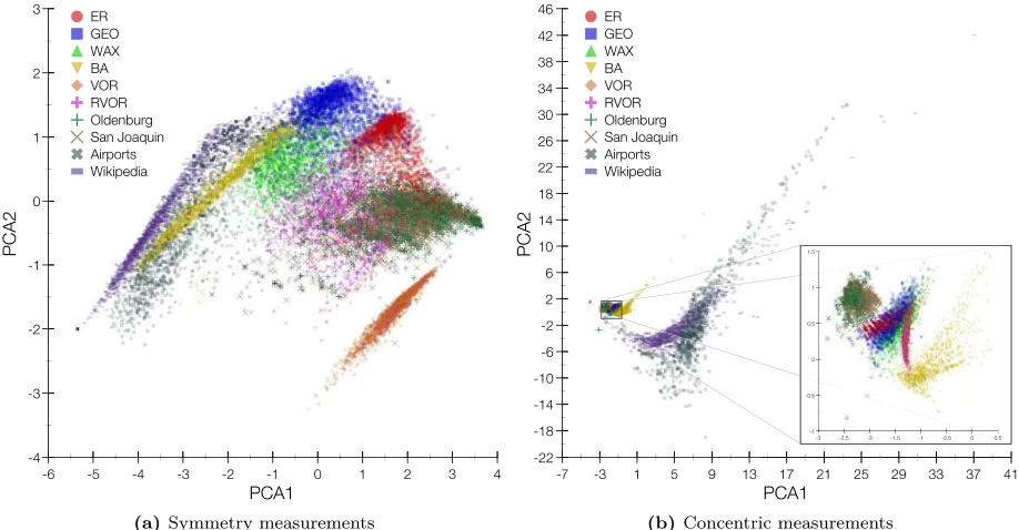
h = 2,3 and 4, this defines a 6-dimensional space con-taining all the selected nodes. The PCA is applied to this data and the first two components are retained, the result is shown in Figure 13(a). The PCA in Figure 13(a) encompasses most of the main results of this paper and highlights the relationships between the symmetric fea-tures of the considered networks. The two first PCA

axes have been verified to account for≈86% of the to-tal variance. The component PCA1 corresponds to a balanced linear combination of all symmetry measure-ments, i.e.PCA1 = 0.37Sb(2)i + 0.43Sm

(2)

i + 0.44Sb

(3)

i +

0.43Sm(3)i +0.43Sb

(4)

i +0.34Sm

(4)

i . Therefore, higher

between themselves even though they share a geograph-ical nature. This might be caused by the existence of long-range connections present in the WAX model, which are not allowed in the GEO networks. Both street net-works presents great overlap in the PCA space and, along PCA1, they are closer to the ER model than to the geo-graphical models. At the same time, the RVOR network presented an even larger overlap with the two cities.

In order to compare the results obtained using the sym-metry measurements, we also applied the PCA consider-ing several more traditional concentric characteristics [22] (e.g. concentric degree, clustering). The result is shown in Figure 13(b). By comparing the two PCA projec-tions, it becomes clear that the symmetry measurements provide a more discriminative representation of the sev-eral considered networks, reflected in less overlap between clusters allied to wider distributions of nodes within the clusters associated to each network. The relatively small overlaps between some of the networks in Figure 13(a), such as between ER and the street networks, are indeed expected. A good deal of such remarkable properties can be understood to be related to the insensitivity of the symmetry measurements to the node degree, which oth-erwise implies in widely different sizes of clusters (see Figure 13(b)).

The spatial dispersion of the node symmetry measure-ments, quantified in terms of the trace of the respective covariance matrix, obtained for the several networks con-sidered in this article, are given in Table I respectively to the concentric levelsh= 2,3,and 4.

In general, the PCA provides an important overview of the symmetry measurements. In addition, the PCA1 axis retains 71% of their variance, this allow us to rank the networks in terms of an overall symmetry value, i.e. PCA1. The most symmetric networks are those of streets, followed by the ER model and the two spatial models. On the other hand, Wikipedia, airports and BA models are the more asymmetrical networks and also pre-senting the higher dispersion values forh= 2(please see Table I). Such ordering alongPCA1 tends to reflect the regularity/simplicity of the original networks, a possibil-ity that needs to be further investigated.

VI. CONCLUSIONS

Complex networks can be studied at different topo-logical scales: local-scale characterized by the connectiv-ity between neighbors of a node, intermediate-scale usu-ally associated to communities; and global-scale concern-ing the overall structure of the network. While several methods have been developed for the characterization of global-scale symmetries in networks, mostly based on au-tomorphism [1, 3], it is also interesting to develop con-cepts and methods capable of quantifying the symmetry more locally, e.g. around a given neighborhood of a node. The concept of symmetry developed in the current ar-ticle is associated to the regularity of the transition

prob-abilities of a concentric random walk. Since the calcula-tions are always done using a single node as a reference, we can relate the concept of topological symmetry with our visual perception of symmetry. This relationship is particularly noticeable for the Erdős-Renyi model (ER). Since connections inside the same concentric levels are uncommon for the ER network, giving rise to a tree-like organization, the topological symmetry is mainly deter-mined by the balance of connections along tree branches. This property also allows for a clear visualization of the topological symmetry.

The Barabási Albert (BA) model provides a nice con-trast to the ER model, since it is highly probable that one or more hubs are accessed after one or two steps from the reference node. This property implies a strong un-balance on the transition probabilities of the concentric random walk, since nodes reached after passing through the hub are accessed with much lower probability than other nodes on the same concentric level that are not as-sociated with hubs. Another interesting network model to be investigated is the spatial model. Since the nodes in these networks have a well-defined position influencing the connectivity of patterns, it is interesting to quantify how this influence translates to topological symmetry.

Regarding the real-world networks, it is interesting that the airport and Wikipedia showed a larger range of symmetry values than any network model. This might happen because the connectivity patterns of the nodes do not follow single rules as in the models, in the sense that they present a hybrid topology. For the airport networks, different countries or states have specific demands (e.g. passenger flow). In the Wikipedia, each subject (i.e., mathematics, biology, etc) tends to present specific cita-tion patterns [23]. Still, the topological patterns are more symmetric than those observed in the models, which is confirmed by higher values of backbone and merged sym-metry. This is probably a consequence of the adjacency constraints implied by planarity that need to be followed in city planning, such as in Voronoi networks [16]. Al-though the GEO network share many similar character-istics with the street networks, they are not specifically made to be navigable.

As developed in this work, the symmetry measurement was found to capture many distinct concentric patterns of connectivity. A natural extension of our analysis is to verify which of these patterns occur more often than it would be expected by chance on real-world networks. Therefore, by analyzing the density of points in the sym-metry space we can identify motifs in the network struc-ture. It would be important to verify how many distinct patterns can be associated to the same pair of symme-try values. Another additional development is to identify typical symmetry patterns specific to distinct regions of the real-world networks. For example, would a given re-gion of the airport network present some intrinsic orga-nization? Or, would given areas of Wikipedia exhibit typical symmetry patterns?

PCA1

PCA2

-6 -5 -4 -3 -2 -1 0 1 2 3 4

-4 -3 -2 -1 0 1 2

3 _ER

GEO WAX BA VOR RVOR Oldenburg San Joaquin Airports Wikipedia

(a)Symmetry measurements

PCA1

-7 -3 1 5 9 13 17 21 25 29 33 37 41

-22 -18 -14 -10 -6 -2 2 6 10 14 18 22 26 30 34 38 42 46

-3 -2.5 -2 -1.5 -1 -0.5 0 0.5 -1

-0.5 0 0.5 1 1.5

PCA2

ER GEO WAX BA VOR RVOR Oldenburg San Joaquin Airports Wikipedia

(b)Concentric measurements

FIG. 13: PCAs obtained from the standardized backbone and merged symmetries from level h= 2to h = 4(a), and from concentric measurements [22] considering the same range of levels (b). Because the networks present distinct number of nodes, only1000nodes randomly sampled from each network are considered for the calculation.

TABLE I: Trace of the covariance matrix calculated for the backbone and merged symmetry values at each concentric level.

Concentric

Level (h) ER GEO WAX Voronoi

Voronoi

(Rewired) BA Oldenburg San Joaquin Airports Wikipedia

2 0.010 0.020 0.044 0.005 0.039 0.112 0.023 0.021 0.182 0.144 3 0.011 0.052 0.034 0.013 0.069 0.021 0.038 0.038 0.081 0.033

4 0.067 0.014 0.022 0.019 0.050 0.005 0.039 0.039 0.040 0.007

All 0.088 0.086 0.100 0.037 0.158 0.138 0.100 0.098 0.303 0.184

disease propagate over the network. Diffusion and disease dynamics are of particular interest since it is possible to analyze how the number of symmetric patterns in the network impacts the speed of a dynamics propagation. This idea is related to some previous results showing that degree heterogeneity can facilitate disease propagation on networks [24, 25].

Acknowledgements

F. N. Silva acknowledges CAPES. C. H. Comin thanks FAPESP (Grant No. 11/22639-8) for financial support. T. K. D. M. Peron acknowledges FAPESP (Grant no.

2012/22160-7) for support. F. A. Rodrigues acknowl-edges CNPq (grant 305940/2010-4), FAPESP (grant 2011/507612 and 2013/264169) and NAP eScience -PRP - USP for financial support. L. da F. Costa thanks CNPq (Grant no. 307333/2013-2) and NAP-PRP-USP for support. This work has been supported also by FAPESP grants 12/50986-7 and 11/50761-2.

Appendix A: Correlation between symmetry and degree

[1] C. Godsil and G. F. Royle, in Algebraic Graph Theory

(Springer, 2001).

0.0 0.1 0.2 0.3 0.4 0.5 0.6 0.7 0.8 0.9 1.0

Backbone Symmetry (h=2) 0.0

0.1 0.2 0.3 0.4 0.5 0.6 0.7 0.8 0.9 1.0

Merged Symmetry (h=2)

0 Node Degree 20

(a)h_{= 2}

0.0 0.1 0.2 0.3 0.4 0.5 0.6 0.7 0.8 0.9 1.0

Backbone Symmetry (h=3) 0.0

0.1 0.2 0.3 0.4 0.5 0.6 0.7 0.8 0.9 1.0

Merged Symmetry (h=3)

0 Node Degree 20

(b)h_{= 3}

0.0 0.1 0.2 0.3 0.4 0.5 0.6 0.7 0.8 0.9 1.0

Backbone Symmetry (h=4) 0.0

0.1 0.2 0.3 0.4 0.5 0.6 0.7 0.8 0.9 1.0

Merged Symmetry (h=4)

0 Node Degree 20

(c)h_{= 4}

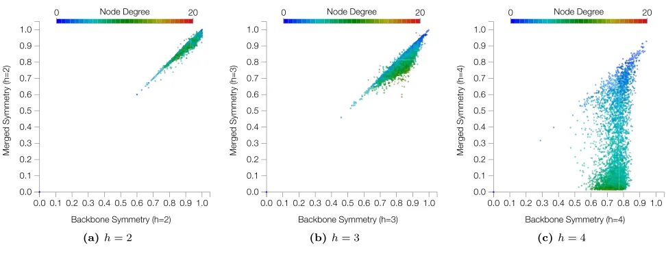
FIG. 14: Scatterplots of backbone vs merged symmetry measurements for the ER network considering concentric levelsh= 2,3

and4. The points are colored according to the degree of the respective node.

0.0 0.1 0.2 0.3 0.4 0.5 0.6 0.7 0.8 0.9 1.0

Backbone Symmetry (h=2) 0.0

0.1 0.2 0.3 0.4 0.5 0.6 0.7 0.8 0.9 1.0

Merged Symmetry (h=2)

1 Node Degree 16

(a)h_{= 2}

0.0 0.1 0.2 0.3 0.4 0.5 0.6 0.7 0.8 0.9 1.0

Backbone Symmetry (h=3) 0.0

0.1 0.2 0.3 0.4 0.5 0.6 0.7 0.8 0.9 1.0

Merged Symmetry (h=3)

1 Node Degree 16

(b)h_{= 3}

0.0 0.1 0.2 0.3 0.4 0.5 0.6 0.7 0.8 0.9 1.0

Backbone Symmetry (h=4) 0.0

0.1 0.2 0.3 0.4 0.5 0.6 0.7 0.8 0.9 1.0

Merged Symmetry (h=4)

1 Node Degree 16

(c)h_{= 4}

FIG. 15: Scatterplots of backbone vs merged symmetry measurements for the GEO network considering concentric levels

h= 2,3and4. The points are colored according to the degree of the respective node.

[3] N. Biggs,Algebraic Graph Theory(Cambridge University Press, 1994).

[4] L. W. Beineke and R. J. Wilson, Topics in Algebraic Graph Theory, vol. 102 (Cambridge University Press, 2004).

[5] Y. Xiao, M. Xiong, W. Wang, and H. Wang, Physical Review E77, 066108 (2008).

[6] P. Holme, Physical Review E74, 036107 (2006). [7] B. D. MacArthur, R. J. Sánchez-García, and J. W.

An-derson, Discrete Applied Mathematics156, 3525 (2008). [8] M. P. Viana, J. L. Batista, and L. da F. Costa, Physical

Review E85, 036105 (2012).

[9] B. A. N. Travençolo, M. P. Viana, and L. d. F. Costa, New Journal of Physics11, 063019 (2009).

[10] B. Travençolo and L. da F Costa, Physics Letters A373, 89 (2008).

[11] L. da F. Costa and F. A. Rodrigues, Europhysics Letters

85, 48001 (2009).

[12] L. da. F. Costa, M. A. R. Tognetti, and F. N. Silva, Physica A387, 6201 (2008).

[13] M. Newman, Networks: An Introduction (Oxford Uni-versity Press, 2010).

[14] J. Dall and M. Christensen, Physical Review E 66, 016121 (2002).

[15] B. M. Waxman, Selected Areas in Communications, IEEE Journal on6, 1617 (1988).

[16] M. Barthélemy, Physics Reports499, 1 (2011).

[17] E. Estrada, The structure of complex networks: theory and applications (Oxford University Press, New York, 2012), ISBN 978-0-19-959175-6.

[18] L. da F. Costa, International Journal of Modern Physics C15, 175 (2004).

[19] T. Brinkhoff, Geoinformatica6, 153 (2002).

0.0 0.1 0.2 0.3 0.4 0.5 0.6 0.7 0.8 0.9 1.0

Backbone Symmetry (h=2) 0.0

0.1 0.2 0.3 0.4 0.5 0.6 0.7 0.8 0.9 1.0

Merged Symmetry (h=2)

0 Node Degree 16

(a)h_{= 2}

0.0 0.1 0.2 0.3 0.4 0.5 0.6 0.7 0.8 0.9 1.0

Backbone Symmetry (h=3) 0.0

0.1 0.2 0.3 0.4 0.5 0.6 0.7 0.8 0.9 1.0

Merged Symmetry (h=3)

0 Node Degree 16

(b)h_{= 3}

0.0 0.1 0.2 0.3 0.4 0.5 0.6 0.7 0.8 0.9 1.0

Backbone Symmetry (h=4) 0.0

0.1 0.2 0.3 0.4 0.5 0.6 0.7 0.8 0.9 1.0

Merged Symmetry (h=4)

0 Node Degree 16

(c)h_{= 4}

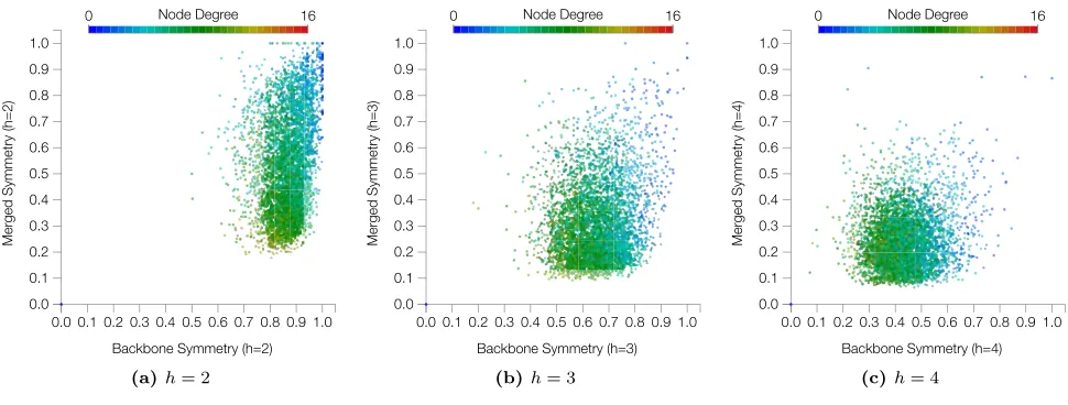
FIG. 16: Scatterplots of backbone vs merged symmetry measurements for the WAX network considering concentric levels

h= 2,3and4. The points are colored according to the degree of the respective node.

0.0 0.1 0.2 0.3 0.4 0.5 0.6 0.7 0.8 0.9 1.0

Backbone Symmetry (h=2) 0.0

0.1 0.2 0.3 0.4 0.5 0.6 0.7 0.8 0.9 1.0

Merged Symmetry (h=2)

2 Node Degree 14

(a)h_{= 2}

0.0 0.1 0.2 0.3 0.4 0.5 0.6 0.7 0.8 0.9 1.0

Backbone Symmetry (h=3) 0.0

0.1 0.2 0.3 0.4 0.5 0.6 0.7 0.8 0.9 1.0

Merged Symmetry (h=3)

2 Node Degree 14

(b)h_{= 3}

0.0 0.1 0.2 0.3 0.4 0.5 0.6 0.7 0.8 0.9 1.0

Backbone Symmetry (h=4) 0.0

0.1 0.2 0.3 0.4 0.5 0.6 0.7 0.8 0.9 1.0

Merged Symmetry (h=4)

2 Node Degree 14

(c)h_{= 4}

FIG. 17: Scatterplots of backbone vs merged symmetry measurements for the VOR network considering concentric levels

h= 2,3and4. The points are colored according to the degree of the respective node.

168703 (2013).

[21] I. T. Jolliffe, Principal component analysis (Springer, 2002).

[22] L. da. F. Costa and F. N. Silva, J Stat Phys 125, 845 (2006).

[23] F. Silva, M. Viana, B. Travençolo, and L. da F. Costa, Journal of Informetrics5, 431 (2011).

[24] R. Pastor-Satorras and A. Vespignani, Physical Review

Letters86, 3200 (2001).

[25] F. J. Pérez-Reche, S. N. Taraskin, W. Otten, M. P. Viana, L. da F. Costa, and C. A. Gilligan, Physical Review Let-ters109, 098102 (2012).

0.0 0.1 0.2 0.3 0.4 0.5 0.6 0.7 0.8 0.9 1.0

Backbone Symmetry (h=2) 0.0

0.1 0.2 0.3 0.4 0.5 0.6 0.7 0.8 0.9 1.0

Merged Symmetry (h=2)

2 Node Degree 14

(a)h_{= 2}

0.0 0.1 0.2 0.3 0.4 0.5 0.6 0.7 0.8 0.9 1.0

Backbone Symmetry (h=3) 0.0

0.1 0.2 0.3 0.4 0.5 0.6 0.7 0.8 0.9 1.0

Merged Symmetry (h=3)

2 Node Degree 14

(b)h_{= 3}

0.0 0.1 0.2 0.3 0.4 0.5 0.6 0.7 0.8 0.9 1.0

Backbone Symmetry (h=4) 0.0

0.1 0.2 0.3 0.4 0.5 0.6 0.7 0.8 0.9 1.0

Merged Symmetry (h=4)

2 Node Degree 14

(c)h_{= 4}

FIG. 18: Scatterplots of backbone vs merged symmetry measurements for the RVOR network considering concentric levels

h= 2,3and4. The points are colored according to the degree of the respective node.

0.0 0.1 0.2 0.3 0.4 0.5 0.6 0.7 0.8 0.9 1.0

Backbone Symmetry (h=2) 0.0

0.1 0.2 0.3 0.4 0.5 0.6 0.7 0.8 0.9 1.0

Merged Symmetry (h=2)

3 Node Degree 173

(a)h_{= 2}

0.0 0.1 0.2 0.3 0.4 0.5 0.6 0.7 0.8 0.9 1.0

Backbone Symmetry (h=3) 0.0

0.1 0.2 0.3 0.4 0.5 0.6 0.7 0.8 0.9 1.0

Merged Symmetry (h=3)

3 Node Degree 173

(b)h_{= 3}

0.0 0.1 0.2 0.3 0.4 0.5 0.6 0.7 0.8 0.9 1.0

Backbone Symmetry (h=4) 0.0

0.1 0.2 0.3 0.4 0.5 0.6 0.7 0.8 0.9 1.0

Merged Symmetry (h=4)

3 Node Degree 173

(c)h_{= 4}

FIG. 19: Scatterplots of backbone vs merged symmetry measurements for the BA network considering concentric levelsh= 2,3

0.0 0.1 0.2 0.3 0.4 0.5 0.6 0.7 0.8 0.9 1.0

Backbone Symmetry (h=2) 0.0

0.1 0.2 0.3 0.4 0.5 0.6 0.7 0.8 0.9 1.0

Merged Symmetry (h=2)

0 Node Degree 216

(a)h_{= 2}

0.0 0.1 0.2 0.3 0.4 0.5 0.6 0.7 0.8 0.9 1.0

Backbone Symmetry (h=3) 0.0

0.1 0.2 0.3 0.4 0.5 0.6 0.7 0.8 0.9 1.0

Merged Symmetry (h=3)

0 Node Degree 216

(b)h_{= 3}

0.0 0.1 0.2 0.3 0.4 0.5 0.6 0.7 0.8 0.9 1.0

Backbone Symmetry (h=4) 0.0

0.1 0.2 0.3 0.4 0.5 0.6 0.7 0.8 0.9 1.0

Merged Symmetry (h=4)

0 Node Degree 216

(c)h_{= 4}

FIG. 20: Scatterplots of backbone vs merged symmetry measurements for the airport network considering concentric levels

h= 2,3and4. The points are colored according to the degree of the respective node.

0.0 0.1 0.2 0.3 0.4 0.5 0.6 0.7 0.8 0.9 1.0

Backbone Symmetry (h=2) 0.0

0.1 0.2 0.3 0.4 0.5 0.6 0.7 0.8 0.9 1.0

Merged Symmetry (h=2)

1 Node Degree 1,320

(a)h_{= 2}

0.0 0.1 0.2 0.3 0.4 0.5 0.6 0.7 0.8 0.9 1.0

Backbone Symmetry (h=3) 0.0

0.1 0.2 0.3 0.4 0.5 0.6 0.7 0.8 0.9 1.0

Merged Symmetry (h=3)

1 Node Degree 1,320

(b)h_{= 3}

0.0 0.1 0.2 0.3 0.4 0.5 0.6 0.7 0.8 0.9 1.0

Backbone Symmetry (h=4) 0.0

0.1 0.2 0.3 0.4 0.5 0.6 0.7 0.8 0.9 1.0

Merged Symmetry (h=4)

1 Node Degree 1,320

(c)h_{= 4}

FIG. 21: Scatterplots of backbone vs merged symmetry measurements for the Wikipedia network considering concentric levels

0.0 0.1 0.2 0.3 0.4 0.5 0.6 0.7 0.8 0.9 1.0

Backbone Symmetry (h=2) 0.0

0.1 0.2 0.3 0.4 0.5 0.6 0.7 0.8 0.9 1.0

Merged Symmetry (h=2)

1.0 Node Degree 5.0

(a)h_{= 2}

0.0 0.1 0.2 0.3 0.4 0.5 0.6 0.7 0.8 0.9 1.0

Backbone Symmetry (h=3) 0.0

0.1 0.2 0.3 0.4 0.5 0.6 0.7 0.8 0.9 1.0

Merged Symmetry (h=3)

1.0 Node Degree 5.0

(b)h_{= 3}

0.0 0.1 0.2 0.3 0.4 0.5 0.6 0.7 0.8 0.9 1.0

Backbone Symmetry (h=4) 0.0

0.1 0.2 0.3 0.4 0.5 0.6 0.7 0.8 0.9 1.0

Merged Symmetry (h=4)

1.0 Node Degree 5.0

(c)h_{= 4}

FIG. 22: Scatterplots of backbone vs merged symmetry measurements for the Oldenburg City network considering concentric levelsh= 2,3and4. The points are colored according to the degree of the respective node.

0.0 0.1 0.2 0.3 0.4 0.5 0.6 0.7 0.8 0.9 1.0

Backbone Symmetry (h=2) 0.0

0.1 0.2 0.3 0.4 0.5 0.6 0.7 0.8 0.9 1.0

Merged Symmetry (h=2)

1 Node Degree 8

(a)h_{= 2}

0.0 0.1 0.2 0.3 0.4 0.5 0.6 0.7 0.8 0.9 1.0

Backbone Symmetry (h=3) 0.0

0.1 0.2 0.3 0.4 0.5 0.6 0.7 0.8 0.9 1.0

Merged Symmetry (h=3)

1 Node Degree 8

(b)h_{= 3}

0.0 0.1 0.2 0.3 0.4 0.5 0.6 0.7 0.8 0.9 1.0

Backbone Symmetry (h=4) 0.0

0.1 0.2 0.3 0.4 0.5 0.6 0.7 0.8 0.9 1.0

Merged Symmetry (h=4)

1 Node Degree 8

(c)h_{= 4}