Defining a 3-dimensional trishear parameter space to understand the temporal evolution of fault propagation folds

This is a repository copy of

Defining a 3-dimensional trishear parameter space to

understand the temporal evolution of fault propagation folds

.

White Rose Research Online URL for this paper:

http://eprints.whiterose.ac.uk/80599/

Version: Supplemental Material

Article:

Pei, Y, Paton, DA and Knipe, RJ (2014) Defining a 3-dimensional trishear parameter space

to understand the temporal evolution of fault propagation folds. Journal of Structural

Geology, 66. 284 - 297. ISSN 0191-8141

https://doi.org/10.1016/j.jsg.2014.05.018

[email protected] https://eprints.whiterose.ac.uk/

Reuse

Unless indicated otherwise, fulltext items are protected by copyright with all rights reserved. The copyright exception in section 29 of the Copyright, Designs and Patents Act 1988 allows the making of a single copy solely for the purpose of non-commercial research or private study within the limits of fair dealing. The publisher or other rights-holder may allow further reproduction and re-use of this version - refer to the White Rose Research Online record for this item. Where records identify the publisher as the copyright holder, users can verify any specific terms of use on the publisher’s website.

Takedown

If you consider content in White Rose Research Online to be in breach of UK law, please notify us by

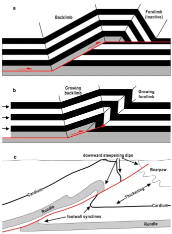
Figure 1. Fault-bend fold and fault-propagation fold based on kink bend method (a, b) 2

(Suppe, 1983; Suppe and Medwedeff, 1990) and a natural example showing variable 3

layer thickness (c) (Allmendinger, 1998). 4

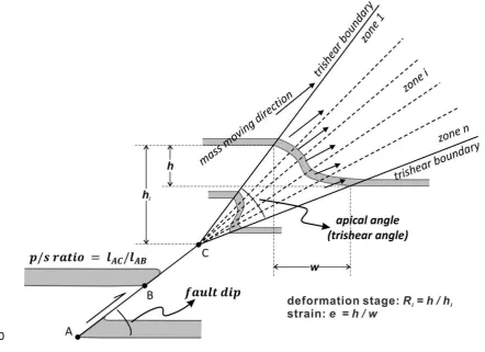
Figure 2. Conceptual model of trishear algorithm, based on Hardy and Ford (1997). 5

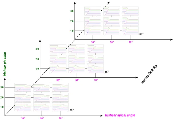
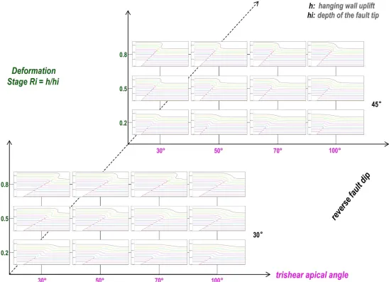
Figure 3. Three-dimensional parameter space with corresponding trishear models. 6

The three axes represent the trishear p/s ratio, the trishear apical angle and the 7

reverse fault dip, respectively. 8

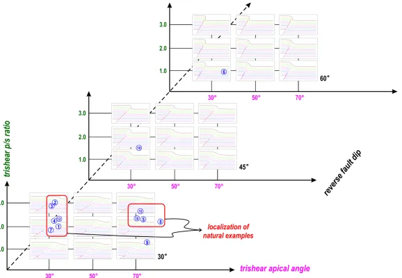
Figure 4. Clusters of natural trishear examples in the three-dimensional parameter 9

space. In the parameter space, 13 natural examples are plotted in and two clusters 10

are observed. The clusters suggest that the most applicable trishear p/s ratio is 2-3 11

and the trishear apical angle varies from 30° to 100°. The majority of these natural 12

trishear examples show shallow fault dips of 25°-45°. 13

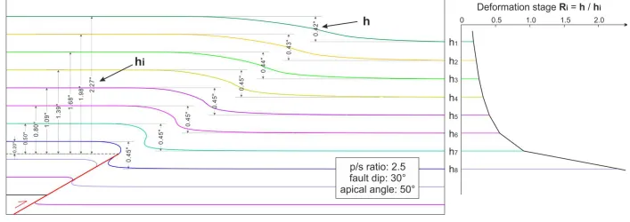
Figure 5. Diagram delineating the impact of the selection of the reference level, i.e., 14

the horizon used to calculate the deformation stage . Here a trishear model (left) 15

with the parameters p/s ratio of 2.5, fault dip of 30° and apical angle of 50° is 16

selected, in which we only calculate the of the horizons that have not been 17

propagated through by the underlying fault. The deformation stage is not unique 18

for a trishear model, but is variable for different horizons. The right diagram suggests 19

a decreasing value from h8 to h1 upward through the model. 20

Figure 6. Parameter space of trishear models with suggested parameters from the 21

clusters of natural trishear examples. 22

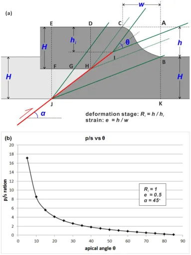
Figure 7. Quantification of strain (ratio of hanging wall uplift versus folded bed width) 23

associated with trishear algorithm. The figure (a) delineates the trigonometric 24

generated with known strain = 0.5, deformation stage = 1 and fault dip = 45° 26

in (b). 27

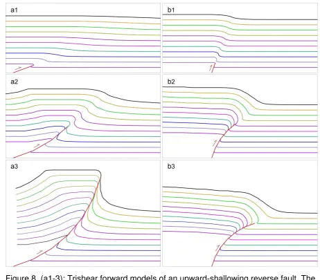
Figure 8. (a1-3): Trishear forward models of an upward-shallowing reverse fault. The 28

fault dip changes from 20° to 70° upwards with a stepwise increment of 10°. (b1-3): 29

Trishear forward models of an upward-shallowing reverse fault. The fault dip changes 30

from 70° to 20° upwards with a stepwise decrement of 10°. 31

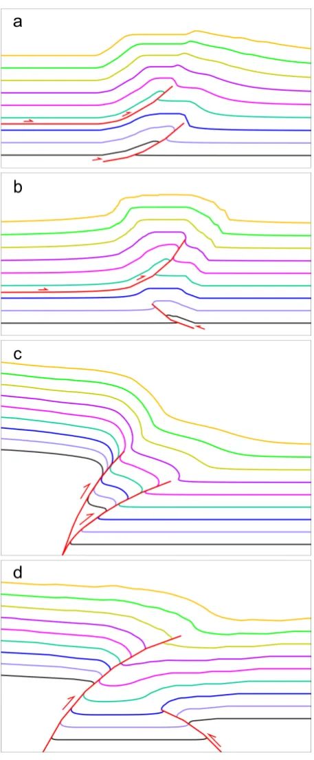
Figure 9. Trishear forward models of reverse faults affected by pre-existing faults. (a 32

& b) upward-steepening reverse faults developed above deeper pre-existing reverse 33

faults. (c & d) upward-shallowing reverse fault developed above deeper pre-existing 34

reverse faults. Pre-existing faults with the same or opposite thrusting directions are 35

all simulated. 36

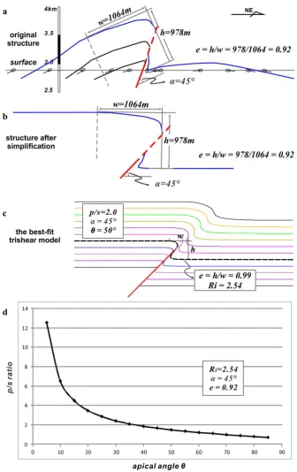
Figure 10. The workflow of applying trishear algorithm to the Lenghu5 structure, 37

Qaidam Basin, Northern Tibetan Plateau. 38

Figure 11. The forward trishear models depicts the structural evolution of the 39

Lenghu5 structure by allowing multiple curved reverse faults in trishear forward 40

modelling. 41

42

Table 1. A cluster of natural trishear examples in published studies and their 43

corresponding best-fit parameters. 44

Figure 1. Fault-bend fold and fault-propagation fold based on kink bend

meth-47

od (a, b)

(Suppe, 1983; Suppe and Medwedeff, 1990)

and a natural example

48

showing variable layer thickness (c)

(Allmendinger, 1998)

.

50

Figure 2. Conceptual model of trishear algorithm, based on

Hardy and Ford

(1997)

.

Figure 3. Three-dimensional parameter space with corresponding trishear models. The three axes represent the trishear p/s ratio,

54

the trishear apical angle and the reverse fault dip, respectively.

56

Figure 4. Clusters of natural trishear examples in the three-dimensional parameter space. In the parameter space, 13 natural

ex-57

amples are plotted in and two clusters are observed. The clusters suggest that the most applicable trishear p/s ratio is 2-3 and the

58

trishear apical angle varies from 30° to 100°. The majority of these natural trishear examples show shallow fault dips of 25°-45°.

Figure 5. Diagram delineating the impact of the selection of the reference level, i.e., the horizon used to calculate the deformation

61

stage

. Here a trishear model (left) with the parameters p/s ratio of 2.5, fault dip of 30° and apical angle of 50° is selected, in

62

which we only calculate the

of the horizons that have not been propagated through by the underlying fault. The deformation

63

stage

is not unique for a trishear model, but is variable for different horizons. The right diagram suggests a decreasing

value

64

from h8 to h1 upward through the model.

66

Figure 6. Parameter space of trishear models with suggested parameters from the clusters of natural trishear examples.

Figure 7. Quantification of strain (ratio of hanging wall uplift versus folded bed width)

69

associated with trishear algorithm. The figure (a) delineates the trigonometric

rela-70

tionship among the variables, while the apical angle versus p/s ratio plot is generated

71

with known strain = 0.5, deformation stage

= 1 and fault dip

= 45° in (b).

73

Figure 8. (a1-3): Trishear forward models of an upward-shallowing reverse fault. The

74

fault dip changes from 20° to 70° upwards with a stepwise increment of 10°. (b1-3):

75

Trishear forward models of an upward-shallowing reverse fault. The fault dip

chang-76

es from 70° to 20° upwards with a stepwise decrement of 10°.

Figure 9. Trishear forward models of reverse faults affected by pre-existing faults. (a

79

& b) upward-steepening reverse faults developed above deeper pre-existing reverse

80

faults. (c & d) upward-shallowing reverse fault developed above deeper pre-existing

81

reverse faults. Pre-existing faults with the same or opposite thrusting directions are

82

all simulated.

84

Figure 10. The workflow of applying trishear algorithm to the Lenghu5 structure,

85

Qaidam Basin, Northern Tibetan Plateau.

hu5 structure by allowing multiple curved reverse faults in trishear forward modelling.

Tables

90

Table 1. A cluster of natural trishear examples in published studies and their corresponding best-fit parameters.

91

Ref

No. Structure names

Basement-involved p/s ratio apical angle fault dip

Scale, fault slip

or stratigraphy Example Sources

1 Turner Valley, Rocky Mountain No 2.0+ 37 25 Scale: 12km*30km (section width*depth); fault slip: 10km;

Hardy and Ford (1997)

2 Tejerina Fault, Spain No 3.0+ 35 30 Scale: 0.8km*1.2km; fault slip: 250m; stratigra-phy: conglomerates with thin shales;

Hardy and Ford (1997)

3 Broad Haven, Pembrokeshire No 3.0+ 35 24 Scale: 6m*10m; fault slip: 2m; Hardy and Ford (1997)

4 Hudson Valley, New York No 2.5 30-35 36 Scale: 2km*3km; fault slip: 0.3km; Allmendinger (1998)

5 Rangely anticline, W US No 2.3 76 38 Scale: 6km*12km; fault slip: 4.2km; Allmendinger (1998)

6 Reelfoot Fault, Proctor, US Yes 0.9 36 80 Scale: 0.5km*0.8km; fault slip: 52m; Champion et al. (2001)

7 Filo Morado structure, W Neuquen basin

No 1.9 35

30-40

Scale: 4km*10km; fault slip: 8.7km; stratigra-phy: thick units (evaporates & shales)

Allmendinger et al. (2004)

8 Waterpocket anticline, S Utah No 2.25 105 35 Scale: 5km*10km; fault slip:3.8km; Cardozo (2005)

9 Rip Van Winkle anticline, New York

No 1.5 90 25 Scale: 5km*8km; fault slip:43m; stratigraphy: wackstone, packstone and grainstone;

Cardozo et al. (2005)

10 Dalong fault, Gansu, China Yes 1.5 30 50 Scale: 5km*10km; fault slip:669m; stratigraphy: basement + cover (terrestrial clastic sediments);

Gold et al. (2006)

11 Chelungpu fault, Taiwan No 2.5 80 35 Scale: 5m*40m; fault slip: 6m; stratigraphy: clay, silt clay with sand;

Lin et al. (2007)

12 Hudson Valley, New York No 2.4 36 35 Scale: 2km*3km; fault slip: 0.3km; Cardozo and

Aanonsen (2009)

13 Santa Fe Springs anticline, Los Angeles basin

No 2.52 71 29 Scale: 7km*12km; fault slip:6.7km; Cardozo and