promoting access to White Rose research papers
White Rose Research Online
eprints@whiterose.ac.uk
Universities of Leeds, Sheffield and York
http://eprints.whiterose.ac.uk/
This is a copy of the final published version of a paper published via gold open access
in
Journal of Biomedical Informatics
.
This open access article is distributed under the terms of the Creative Commons
Attribution Licence (http://creativecommons.org/licenses/by/3.0), which permits
unrestricted use, distribution, and reproduction in any medium, provided the
original work is properly cited.
White Rose Research Online URL for this paper:
http://eprints.whiterose.ac.uk/76883
Published paper
McInnes, B and Stevenson, R.M (2013) Determining the Difficulty of Word Sense
Disambiguation. Journal of Biomedical Informatics, 47. pp. 83-90.Doi:
Determining the difficulty of Word Sense Disambiguation
Bridget T. McInnes
a,⇑, Mark Stevenson
ba
Minnesota Supercomputing Institute, University of Minnesota, 117 Pleasant St SE, Minneapolis, MN 55455, USA
b
Natural Language Processing Group, Department of Computer Science, University of Sheffield, Regent Court, 211 Portobello, Sheffield S1 4DP, United Kingdom
a r t i c l e
i n f o
Article history:
Received 18 February 2013 Accepted 13 September 2013 Available online 26 September 2013
Keywords:
Natural Language Processing NLP
Word Sense Disambiguation WSD
Ambiguity
Biomedical documents
a b s t r a c t
Automatic processing of biomedical documents is made difficult by the fact that many of the terms they contain are ambiguous. Word Sense Disambiguation (WSD) systems attempt to resolve these ambiguities and identify the correct meaning. However, the published literature on WSD systems for biomedical doc-uments report considerable differences in performance for different terms. The development of WSD sys-tems is often expensive with respect to acquiring the necessary training data. It would therefore be useful to be able to predict in advance which terms WSD systems are likely to perform well or badly on.
This paper explores various methods for estimating the performance of WSD systems on a wide range of ambiguous biomedical terms (including ambiguous words/phrases and abbreviations). The methods include both supervised and unsupervised approaches. The supervised approaches make use of informa-tion from labeled training data while the unsupervised ones rely on the UMLS Metathesaurus. The approaches are evaluated by comparing their predictions about how difficult disambiguation will be for ambiguous terms against the output of two WSD systems. We find the supervised methods are the best predictors of WSD difficulty, but are limited by their dependence on labeled training data. The unsu-pervised methods all perform well in some situations and can be applied more widely.
Ó2013 The Authors. Published by Elsevier Inc. This is an open access article under the CC BY license (http://creativecommons.org/licenses/by/3.0/).
1. Introduction
Word Sense Disambiguation(WSD) is the task of automatically identifying the appropriate sense of an ambiguous word based on the context in which the word is used. For example, the term coldcould refer to thetemperatureor thecommon cold, depending on how the word is used in the sentence. Automatically identifying the intended sense of ambiguous words improves the performance of biomedical and clinical applications such as medical coding and indexing; applications that are becoming essential tasks due to the growing amount of information available to researchers.
A wide range of approaches have been applied to the problem of WSD in biomedical and clinical documents[1–7]. Accurate WSD can improve the performance of biomedical text processing appli-cations, such as summarization[8], but inaccurate WSD has been shown to reduce an application’s overall performance[9]. The dis-ambiguation of individual terms is important since some of those terms are more important than others when determining whether there is any overall improvement of the system [8]. The
importance of WSD is likely to depend on the application and re-search question. For example, Weeber et al. [10] found that it was necessary to resolve the ambiguity in the abbreviation ‘‘MG’’ (which can mean ‘‘magnesium’’ or ‘‘milligram’’) in order to repli-cate the connection between migraine and magnesium identified by Swanson[11].
It is now possible to perform very accurate disambiguation for some types of ambiguity, such as abbreviations [12]. However, there is considerable difference in the performance of WSD sys-tems for different ambiguities. For example, Humphrey et al.[3] re-port that the performance of their unsupervised WSD approach varies between 100% (for terms such ascultureanddetermination) and 6% (forfluid). Consequently, it is important to determine the accuracy of a WSD system for the ambiguities of interest to get an idea of whether it will be useful for the overall application, and if so, which terms should be disambiguated.
Historically, supervised machine learning approaches have been shown to disambiguate terms with a higher degree of accuracy than unsupervised methods. The disadvantage to supervised meth-ods is that they require manually annotated training data for each term that needs to be disambiguated. However, manual annotation is an expensive, difficult and time-consuming process which is not practical to apply on a large scale [13]. To avoid this problem, techniques for automatically labeling terms with senses have
http://dx.doi.org/10.1016/j.jbi.2013.09.009
1532-0464/Ó2013 The Authors. Published by Elsevier Inc.
This is an open access article under the CC BY license (http://creativecommons.org/licenses/by/3.0/).
⇑ Corresponding author.
E-mail addresses: btmcinnes@gmail.com (B.T. McInnes), m.stevenson@dcs. shef.ac.uk(M. Stevenson).
Contents lists available atScienceDirect
Journal of Biomedical Informatics
been developed[12,14] but these can only be applied to limited types of ambiguous terms, such as abbreviations and terms which occur with different MeSH codes. Therefore, it would be useful to be able to predict the difficulty of a particular term in order to determine whether applying WSD would be of benefit to the over-all system.
This paper explores approaches to estimating the difficulty of performing WSD on ambiguities found in biomedical documents. By difficulty we mean the WSD performance that can be obtained for the ambiguity since, in practise, performance is the most important factor in determining whether applying WSD to a partic-ular ambiguity is likely to be useful. Ambiguities for which low WSD performance is obtained are considered to be difficult to dis-ambiguate while those for which the performance is high are con-sidered to be easy to disambiguate.
Some of the methods applied in this paper are supervised since they are based on information derived from a corpus containing examples of the ambiguous term labeled with the correct sense. Other methods do not require this resource and only require infor-mation about the number of possible senses for each ambiguous term which is normally obtained from a knowledge source, such as the UMLS Metathesaurus (see Section2.1.1).
Section 2 provides background information on relevant re-sources and techniques for computing similarity or relatedness in the biomedical domain. Section3 describes a range of methods for estimating WSD difficulty, including ones that have been used previously and an unsupervised method based on the similarity/ relatedness measures described in Section2. Experiments to eval-uate these are described in Section4and their results in Section5. Finally, conclusions are presented in Section6.
2. Resources and background
2.1. Resources
This section presents the resources that are used in the experi-ments described later in the paper. In particular, they are used by the similarity and relatedness measures described in Sections2.2.1 and 2.2.2.
2.1.1. Unified Medical Language System
The Unified Medical Language System (UMLS) is a repository that stores a number of distinct biomedical and clinical re-sources. One such resource, used in this work, is the Metathe-saurus [15].
The Metathesaurus contains biomedical and clinical concepts from over 100 disparate terminology sources that have been semi-automatically integrated into a single resource containing a wide range of biomedical and clinical information. For example, it contains the Systematized Nomenclature of Medicine–Clinical Terms (SNOMED CT), which is a comprehensive clinical terminol-ogy created for the electronic exchange of clinical health informa-tion, the Foundational Model of Anatomy (FMA), which is an ontology of anatomical concepts created specifically for biomedical and clinical research, and MedlinePlus Health Topics, which is a terminology source containing health related concepts created specifically for consumers of health services.
The concepts in these sources can overlap. For example, the concept Cold Temperatureexists in both SNOMED CT and MeSH. The Metathesaurus assigns the synonymous concepts from the var-ious sources Concept Unique Identifiers (CUIs). Thus both theCold Temperatureconcepts in SNOMED CT and MeSH are assigned the same CUI (C0009264). This allows multiple sources in the Metathe-saurus to be treated as a single resource.
Some sources in the Metathesaurus contain additional informa-tion such as a concept’s synonyms, its definiinforma-tion,1and its related
concepts. The Metathesaurus contains a number of relations. The two main hierarchical relations are: the parent/child (PAR/CHD) and broader/narrower (RB/RN) relations. A parent/child relation is a hierarchical relation between two concepts that has been explicitly defined in one of the sources. For example, the conceptCold Temper-aturehas an is-arelation with the conceptFreezingin MeSH. This relation is carried forward to the CUI level creating a parent/child relations between the CUIs C0009264 [Cold Temperature] and C0016701 [Freezing] in the Metathesaurus. A broader/narrower rela-tion is a hierarchical relarela-tion that does not explicitly come from a source but is created by the UMLS editors. For this work, we use the parent/child relations.
2.1.2. MEDLINE
MEDLINE2 is a bibliographic database that currently contains
over 22 million citations to journal articles in the biomedical domain and is maintained by the National Library of Medicine (NLM). The 2009 MEDLINE Baseline Repository3 encompasses approximately
5200 journals starting from 1948 and contains 17,764,826 citations; consisting of 2,490,567 unique unigrams (single words) and 39,225,736 unique bigrams (two-word sequences). The majority of the publications are scholarly journals but a small number of other sources such as newspapers and magazines are included.
2.1.3. UMLSonMedline
UMLSonMedline, created by NLM, consists of concepts from the 2009AB UMLS and the number of times they occurred in a snap-shot of MEDLINE taken on 12/01/2009. The frequency counts were obtained by using the Essie Search Engine [16] which queried MEDLINE with normalized strings from the 2009AB MRCONSO ta-ble in the UMLS. The frequency of a CUI was obtained by aggregat-ing the frequency counts of the terms associated with the CUI to provide a rough estimate of its frequency.
2.1.4. Medical Subject Headings (MeSH)
The Medical Subject Headings (MeSH) Thesaurus ([17]) is the NLM’s controlled vocabulary thesaurus consisting of biomedical and health related terms/concepts created for the purpose of indexing articles from MEDLINE. Each MEDLINE citation is associ-ated with a set of manually annotassoci-ated MeSH terms that describe the content of the article. The MeSH terms are organized in a hier-archical structure in order to permit searching at various levels of specificity. The 2013 version contains 26,853 terms organized into 11 different hierarchies.4
2.2. Measures of similarity and relatedness
This section described measures of similarity and relatedness between biomedical concepts that have been previously explored in the literature.
2.2.1. Similarity measures
Existing semantic similarity measures can be categorized into two groups: path-based and information content (IC)-based. Path-based measures use information about the number of nodes between concepts in a hierarchy, whereas IC-based measures incorporate the probability of the concept occurring in a corpus of text.
1
Not all concepts in the UMLS have a definition. 2http://www.ncbi.nlm.nih.gov/pubmed/. 3
http://mbr.nlm.nih.gov/. 4
Path-based Similarity MeasuresRada et al.[18]introduce the conceptual distance measure which is the length of the shortest path between two concepts (c1 andc2) in MeSH using RB/RN rela-tions from the UMLS. Caviedes and Cimino[19]later adapted this measure using the PAR/CHD relations in the UMLS.
Our first measure,path, is a modification of Caviedes and Cimi-no’s approach. Similarity is defined as the reciprocal of the length of the shortest path between the two concepts in the UMLS hierar-chy. This is shown in Eq.(1), wherepath_length(c1,c2) is the number
of nodes in the shortest path betweenc1andc2.
simpathðc1;c2Þ ¼
1 path lengthðc1;c2Þ
ð1Þ
Wu and Palmer [20] extend this measure by incorporating the depth of the Least Common Subsumer (LCS). The LCS of a pair of concepts is the lowest concept in the hierarchy which subsumes that pair. In this measure, the similarity is twice the depth of the two concepts LCS divided by the product of the depths of the indi-vidual concepts as defined in Eq.(2), wheredepthis the number of nodes betweencand the root node in the hierarchy.
simwupðc1;c2Þ ¼
2depthðlcsðc1;c2ÞÞ
depthðc1Þ þdepthðc2Þ
ð2Þ
IC-based Similarity MeasuresInformation content (IC) is for-mally defined as the negative log of the probability of a concept
[21]. The probability of a concept,c, is obtained by summing the number of times it or one of its descendants is seen in a corpus. The concepts descendants are obtained from some concept hierar-chy, such as one of those contained in the UMLS Metathesaurus. Very general concepts have high probabilities since their descen-dants are mentioned frequently and this leads to them having low IC values. Conversely, specific concepts have low probabilities and high IC values. Resnik[22]modified IC for use as a similarity measure. He defined the similarity of two concepts to be the IC of their LCS, see Eq.(3).
simresðc1;c2Þ ¼ICðlcsðc1;c2ÞÞ ¼ logðPðlcsðc1;c2ÞÞÞ ð3Þ
Jiang and Conrath[23]and Lin[24]extended Resnik’s IC-based measure by incorporating the IC of the individual concepts. Lin de-fined the similarity between two concepts by taking the quotient between twice the IC of the concepts’ LCS and the sum of the IC of the two concepts as shown in Eq.(4). This is similar to the mea-sure proposed by Wu and Palmer; differing in the use of IC rather than the depth of the concepts.
simlinðc1;c2Þ ¼
2ICðlcsðc1;c2ÞÞ
ICðc1Þ þICðc2Þ
ð4Þ
Jiang and Conrath defined the distance between two concepts to be the sum of the IC of the two concepts minus twice the IC of the concepts’ LCS. This measure is often modified to return a similarity score by taking the reciprocal of the distance as shown in Eq.(5).
simjcnðc1;c2Þ ¼
1
ICðc1Þ þICðc2Þ 2ICðlcsðc1;c2ÞÞ
ð5Þ
2.2.2. Relatedness measures
Lesk[25]introduces a measure that determines the relatedness between two concepts by counting the number of shared terms in their definitions. An overlap is the longest sequence of one or more consecutive words that occur in both definitions. When imple-menting this measure in WordNet, Banerjee and Pedersen [26]
found that the definitions were short, and did not contain enough overlaps to distinguish between multiple concepts. They extended this measure by including the definition of related concepts in WordNet.
Patwardhan and Pedersen[27]extend the measure proposed by Lesk using second-order co-occurrence vectors. In this method, a vector is created for each word in the concepts definition contain-ing words that co-occur with it in a corpus. These word vectors are average to create a single co-occurrence vector for the concept. The similarity between the concepts is calculated by taking the cosine between the concepts second-order vectors.
3. Estimating WSD difficulty
3.1. Previous approaches
There has been little previous work on estimating the difficulty of WSD. Kilgarriff and Rosenzweig[28]analysed the difficulty of disambiguating terms used in the first SemEval WSD evaluation exercise[29] and found the entropy of the sense distribution to work well. This is calculated as follows:
EntropyðSÞ ¼ X
N
i¼1
PrðsiÞlog2PrðsiÞ ð6Þ
whereS= {s1,s2. . .sN} is the set of possible senses for some
ambig-uous term and Pr (si) the probability of senseSiobtained from a
la-beled corpus.
In domain-independent WSD the Most Frequent Sense (MFS) is commonly used to indicate the difficulty of a particular term
[30,31]. MFS is simply the sense that is found most frequently in a training corpus and is computed as follows:
MFSðSÞ ¼arg max
i PðsiÞ ð7Þ
MFS is often used as a simple baseline for supervised WSD systems
[32]. Like entropy, MFS also requires labeled training data. Both of these approaches are based on the distribution of senses in text and the assumption behind them is that this information is a useful predictor of the difficulty of disambiguating that term. For example, consider an ambiguity where one of the senses is much more likely to appear than the others. The ambiguity will probably be easy to disambiguate, since always assigning the most probable sense will lead to reasonable WSD performance.
Stevenson and Guo[33]applied entropy and MFS to analyse the difficulty of automatically generating labeled WSD training data. However they did not explore whether they could be used to deter-mine the difficulty of WSD for particular terms.
Stevenson and Guo[33]also made use of additional measures. One was the number of possible senses for the ambiguous term. The advantages of this measure is that it is very simple to compute and does not require any labeled training data. The intuition be-hind this approach is that ambiguities with a large number of pos-sible senses will be difficult to disambiguate, simply because of the number of senses to choose from.
3.2. Pairwise similarity
Stevenson and Guo[33]also describe an approach that relies on computing the average pairwise similarity between the possible senses of ambiguous terms (see Section2.2.1). Like counting the number of possible senses, this approach also has the advantage of not requiring any labeled training data.
We extend this approach by considering the maximum simi-larity between senses in addition to the average. Two metrics were applied: mean similarity and maximum similarity. For the mean similarity, the degree of similarity between the concepts of each of the ambiguous word’s possible senses is computed and combined by taking the mean of the similarities. This is calculated as follows:
mean similarityðSÞ ¼
P
fsi;sjg S2 simðsi
;sjÞ
S 2
ð8Þ
whereSis the set of senses andsim(si,sj) is the similarity between
two of these senses as determined by one of the measures described in Section2.2.
Themaximum similaritymeasure is computed in a similar way. However, instead of taking the mean of the pairwise similarities the maximum is chosen:
max similarityðSÞ ¼argmax
fsi;sjg 2S
simðsi;sjÞ ð9Þ
3.3. Implementation
The 2009AB version of the Metathesaurus was used for the experiments described in Section 4. The pairwise similarity ap-proaches described in Section 3.2 are implemented using the UMLS::Similarity package[35], a freely available open source Perl package.5Path information is obtained using the parent/child
rela-tions throughout the entire UMLS. The probabilities required by the IC-based measures are generated using the UMLSonMedline dataset. For the relatedness measures, the definition information is obtained from the concept definitions, as well as the definitions of its parent, child, narrower and broader relations, and its associated terms.
3.4. Example
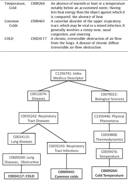
[image:5.595.301.550.99.450.2] [image:5.595.32.287.594.730.2]In this section, we step through an example using the ambigu-ous term cold. In the UMLS, the possible senses forcold include Temperature, Cold [C0009264], the Common Colds [C0009443], or Chronic Obstructive Airways Disease [C0024117]; also referred to as the acronym COLD (Chronic Obstructive Lung Disease).
Table 1shows some of the UMLS Definitions for each of the above senses andFig. 1shows the CUIs and paths between each of the senses. The mean similarity forcoldis calculated by first summing the similarity scores of each combination of senses and dividing it by its number of combinations. An example, using the path mea-sure (see Section2.2.1), is as follows:
mean similarity ¼
P
x;y S
2
sim
ð
x
;
y
Þ
S
2
!
¼simðC0009264;C0009443Þ
þsimðC0009264;C0024117Þ þsimðC0009443;C0024117Þ
3
2
!
¼0:1111þ0:1111þ0:25
3
2
! ¼0:4111
3
2
! ¼0:1574 ð10Þ
4. Evaluation
We evaluated the approaches by determining how well they predict the accuracy of a WSD system on a set of ambiguous terms. Two WSD systems were used in our experiments: one supervised
[36] (see Section 4.1.1) and one unsupervised [37] (see Section4.1.2).
The accuracy of each approach was determined by ranking the terms using the approach and then comparing this with another ranking based on the accuracy of the WSD system. We compared the rankings using Spearman’s Rank Correlation (
q
). Spearman measures the statistical dependence between two variables to as-sesses how well the relationship between the rankings of the vari-ables can be described using a monotonic function. Spearman’s Rank Correlation was used rather than Pearson’s because Pearson’s assumes that the relationship between the data is linear. We used Fisher’s r-to-z transformation to calculate the significance between the correlation results.4.1. Word sense disambiguation
4.1.1. Supervised method
The supervised WSD system developed by Stevenson et al.[36]
combines linguistic and biomedical specific features in a Vector
Table 1
Definitions of the possible senses ofcold.
Term UMLS CUI Example UMLS Definitions Temperature,
Cold
C009264 An absence of warmth or heat or a temperature notably below an accustomed norm; Having less heat energy than the object against which it is compared; the absence of heat
Common Colds
C009443 A catarrhal disorder of the upper respiratory tract, which may be viral or a mixed infection. It generally involves a runny nose, nasal congestion, and sneezing
COLD C0024117 A chronic, irreversible obstruction of air flow from the lungs. A disease of chronic diffuse irreversible air-flow obstruction
Fig. 1.Relationship between three senses of the termcoldin the UMLS (2009AB version). Parent/child relations in the MeSH hierarchy are shown (e.g. C1256751 ‘Topical descriptor’ is parent of C0012674 ‘Diseases’ and C2930671 ‘Phenomena and Process’).
5
http://search.cpan.org/dist/UMLS-Similarity/.
Space Model ([38]). A binary feature vector is created for each pos-sible sense of the ambiguous term and the ambiguous term itself. A range of features are used including local collocations, salient bi-grams, unigrams and MeSH terms. Local collocations are bigrams or trigrams containing the ambiguous term constructed from lem-mas, word forms or part of speech tags. Salient bigrams are those bigrams with a high log likelihood score. Unigrams are lemmas of all content words in the sentence containing the ambiguous term. MeSH terms are indexing terms that had been manually as-signed to each abstract for the purpose of indexing (see Section2). The sense of an ambiguous term is determined by computing the cosine between the vector representing the ambiguous term each of the vectors representing the senses. The sense whose vec-tor has the smallest angle between it and the ambiguous term’s vector is chosen as its most likely sense.
4.1.2. Unsupervised method
We also used the unsupervised WSD system developed by McInnes et al.[37]. In their method, a second-order co-occurrence vector is created for each possible sense of the ambiguous term and the ambiguous term itself. The appropriate sense of the term is then determined by computing the cosine between the vector rep-resenting the ambiguous term and each of the vectors reprep-resenting the sense. The sense whose vector has the smallest angle between it and the ambiguous term’s vector is chosen as the most likely sense.
The vector for a specific sense is created by first obtaining a tex-tual description of the possible sense. This consists of its definition, the definition of its parent/children and narrow/broader relations and the terms associated with the sense from the UMLS. Second, a word by word co-occurrence matrix is created where the rows represent the content words in the description and the columns represent words that co-occur with the words in the description found in MEDLINE abstracts. Lastly, each word in the sense’s description is replaced by its corresponding vector, as given in the co-occurrence matrix. The average of these vectors constitutes the second order co-occurrence vector used to represent the sense. The second-order co-occurrence vector for the ambiguous term is created in a similar fashion by using the words surrounding the ambiguous term in the instance as its textual description.
4.2. Data
Evaluation was carried out using three data sets that include a range of ambiguous terms and abbreviations found in biomedical documents.
4.2.1. Abbreviation dataset
The ‘‘Abbrev’’ dataset6[39]contains examples of 300 ambiguous
abbreviations found in MEDLINE that were initially presented by Liu et al.[40]. The data set was automatically re-created by identifying the abbreviations and long-forms in MEDLINE abstracts and replac-ing the long-form in the abstract with its abbreviation [39]. The abbreviations long-forms were manually mapped to concepts in the UMLS.
4.2.2. NLM-WSD dataset
The National Library of Medicine’s Word Sense Disambiguation (NLM-WSD) dataset7contains 50 frequently occurring ambiguous
words from the 1998 MEDLINE baseline[41]. Each ambiguous word in the NLM-WSD dataset contains 100 ambiguous instances ran-domly selected from the 1998 abstracts totaling to 5000 instances.
The instances were manually disambiguated by 11 evaluators who assigned the ambiguous word to a concept in the UMLS (CUI) or as-signed the concept as ‘‘None’’ if none of the possible concepts de-scribed the term.
4.2.3. MSH-WSD dataset
The National Library of Medicine’s MSH Word Sense Disambig-uation (MSH-WSD) dataset8 contains 203 ambiguous terms and abbreviations from the 2010 MEDLINE baseline [14]. Each target word contains approximately 187 instances, has 2.08 possible senses and has a 54.5% majority sense. Out of 203 target words, 106 are terms, 88 are abbreviations, and 9 have possible senses that are both abbreviations and terms. For example, the target wordcoldhas the abbreviationChronic Obstructive Airway Diseaseas a possible sense, as well as the termCold Temperature. The total number of instances is 37,888.
5. Results and discussion
[image:6.595.312.563.86.156.2]5.1. WSD performance and corpus statistics
Table 2 shows the disambiguation accuracy of the WSD sys-tems for each of the datasets (Abbrev, NLM-WSD and MSH-WSD) and their combination (Combine). The results show that overall the supervised system obtains higher disambiguation accuracies than the unsupervised one, which is consistent with previous results, for example[4–7]. They also show that the accu-racy on the Abbrev dataset is higher than the MSH-WSD or NLM-WSD datasets. We believe this is because the Abbrev dataset con-tains only abbreviations, which have a more coarse grained dis-tinction between their senses. We also see this between the MSH-WSD and NLM-WSD datasets. NLM-WSD primarily contains terms where, as mentioned above, MSH-WSD contains a mix of terms and abbreviations. This explains why the WSD systems ob-tain a higher disambiguation accuracy on the MSH-WSD dataset than the NLM-WSD dataset.
Table 2also shows statistics for all three corpora, the average number of senses per ambiguous term (# Senses), the average MFS and the average entropy. There is not much variation in the average number of senses, with the number varying between 2.1 for MSH-WSD and 2.6 for NLM-WSD. The NLM-WSD dataset has the highest MFS and lowest entropy of the three corpora while the opposite is true for MSH-WSD. The differences in these statis-tics are due to the way in which these datasets were constructed. The NLM-WSD and Abbrev dataset use the sense distributions that are found in corpora which are often highly skewed. For example, all of the instances containing the term associationin the NLM-WSD dataset are annotated with the same sense. However, the MSH-WSD dataset was created by selecting roughly the same number of examples of each possible sense. Consequently informa-tion about the sense distribuinforma-tion is less useful for MSH-WSD than it is for the other datasets.
Table 2
Corpus statistics and overall disambiguation accuracies of WSD systems. Dataset WSD Corpus statistics
Unsupervised Supervised # Senses MFS Entropy NLM-WSD 0.52 0.91 2.3 0.78 0.45 Abbrev 0.91 0.98 2.6 0.70 0.82 MSH-WSD 0.78 0.97 2.1 0.54 1.00 Combined 0.75 0.96 2.10 0.67 0.89
6
http://nlp.shef.ac.uk/BioWSD/downloads/corpora. 7
The NLM-WSD and MSH-WSD (Section4.2.3) datasets are available fromhttp://
wsd.nlm.nih.gov. 8
5.2. Results for previous approaches
Table 3shows the Spearman’s Rank Correlations obtained when the WSD difficulty measures presented in Section3.1were com-pared against the WSD systems.
Overall these measures are better at predicting the accuracy of supervised WSD systems than unsupervised ones. For the NLM-WSD dataset there are high correlations between the accuracy of supervised WSD and two statistics (MFS and entropy). However, this is not surprising since both of these measures make use of information about the distribution of senses in labeled data, and this is the same data that is used to train the WSD system. Corre-lations using these measures are lower for the other two corpora, which have more balanced sense distributions.
Although the number of senses is not a good indicator of super-vised WSD accuracy, it is better than the other measures at predict-ing unsupervised WSD accuracy on the NLM-WSD and Abbrev datasets. The MFS and entropy measures are not effective at pre-dicting unsupervised WSD accuracy, presumably because the unsupervised WSD approaches do not make use of labeled training data.
This analysis suggests that measures such as MFS and entropy are strong indicators of WSD accuracy under some conditions, namely when the WSD system is supervised and the distribution of senses is skewed. However, both of these measures rely on la-beled training data. Consequently they are not useful for predicting the accuracy of supervised WSD systems since the labeled data they require could simply be used to train a WSD model and the accuracy computed directly.
5.3. Results for similarity and relatedness measures
[image:7.595.302.554.538.618.2]The pairwise measures (Section3.2) were evaluated using the measures of similarity and relatedness described in Section2.2.
Table 4shows the Spearman’s Rank Correlation results of the mean (Mean) and maximum (Max) similarity metrics compared to the accuracies from the supervised and unsupervised WSD systems for the combined data set. A positive correlation signifies that as the values of one variable increase, the values of the second vari-able also increase; a negative correlation signifies that as the val-ues of one variable are increasing the other is decreasing. Our hypothesis is that the higher the similarity score the harder it is to disambiguate the ambiguous word. If this is true, we expect that terms with a high similarity score would have a lower disambigu-ation accuracy. Therefore, if the accuracies and the similarity scores of the ambiguous words in the datasets were correlated ex-actly we would see a correlation of 1.0 (exact negative correlation).
Table 5shows thep-values obtained from comparing the max-similarity results using the Fisherr–ztransform. Comparison be-tween the measures using the supervised correlation results are in the upper triangle of the matrix and the unsupervised correla-tion results are in the lower triangle. (Thep-valuesobtained using the mean-similarity are similar.) Allp-values lower than 0.05 are considered to be significant and are printed in bold font.
The results show that the relatedness measureleskobtains a statistically significantly higher negative correlation than the other measures (p60.05). The lesk measure quantifies the similarity
tween the possible senses of a target word based on the overlap be-tween the terms in their definitions. The results indicate that this is a better indicator of how difficult the senses are to distinguish be-tween than the path information obtained from a taxonomy.
The results using the IC-based measures (res,jcnandlin) and the path measure (path) are comparable; there is no statistical differ-ence between the scores (pP0.26). The path measure quantifies the degree of similarity between two concepts using the shortest path information. The IC-based measures extend this, by incorpo-rating the probability of a concept occurring in a corpus. These re-sults indicate extra information about the probability of a concept is not useful for determining the degree of WSD difficulty.Table 6
shows the top five least and most difficult terms to disambiguate and their scores using the Lin with the Mean Similarity Metric. For example, the term cardiac pacemakerhas a similar score of 0.0004 indicating that the similarity between its possible concepts is low making it easier to distinguish between the senses. This is
Table 3
Correlations with WSD accuracy.
Dataset Measure WSD
Unsupervised Supervised NLM-WSD # Senses 0.30 0.17
MFS 0.15 0.89
Entropy 0.17 0.88
Abbr # Senses 0.46 0.14
MFS 0.18 0.57
Entropy 0.33 0.32
MSH-WSD # Senses 0.05 0.06
MFS 0.11 0.14
Entropy 0.11 0.17
Combined # Senses 0.11 0.11
MFS 0.05 0.03
[image:7.595.32.282.651.750.2]Entropy 0.03 0.09
Table 4
Spearman’s rank correlation results over the combined set.
Category Measure Unsupervised Supervised Mean Max Mean Max Path-based path 0.16 0.19 0.21 0.24
wup 0.09 0.11 0.05 0.07 IC-based res 0.10 0.12 0.17 0.18 jcn 0.18 0.19 0.27 0.27 lin 0.15 0.16 0.23 0.23 Relatedness a-lesk 0.33 0.33 0.48 0.49
vector 0.06 0.09 0.18 0.23
Table 5
Significance of spearman’s rank correlations over the combined set for max similarity. Measure path wup res jcn lin a-lesk vector path 0.03 0.26 0.33 0.47 0.0006 0.47 wup 0.18 0.10 0.28 0.03 0.0000 0.03
res 0.20 0.48 0.14 0.29 0.0000 0.56 jcn 0.47 0.20 0.22 0.30 0.0023 0.30 lin 0.34 0.31 0.33 0.38 0.0004 0.50 lesk 0.05 0.005 0.006 0.04 0.02 0.0006
[image:7.595.302.554.679.753.2]vector 0.13 0.41 0.38 0.14 0.23 0.003
Table 6
Top 5 least and most difficult terms to disambiguate using lesk with the mean similarity.
Least Difficult Most Difficult
Term Score Term Score
cardiac pacemaker 0.0004 aa 1.9448
cda 0.0004 fat 1.9713
extraction 0.0005 secretion 1.9910 determination 0.0007 radiation 2.2477
surgery 0.0007 fluid 2.8214
contrary toaawhich has a similarity score of 1.9448 indicating that the similarity between its possible senses are high making it more difficult to distinguish between them.
The path-based measure,wup, quantifies the degree of similar-ity based on the depth of the concepts in the hierarchy. The depth signifies the specificity of a concept; the deeper the concept the more specific it is. The results usingwupshow the correlation to the disambiguation accuracies are random, indicating that using the specificity of the possible senses of a word does not indicate the degree of difficulty to disambiguate it.
The relatedness measure (vector) quantifies the relatedness be-tween the possible senses by looking at the context that surrounds the terms that surround the ambiguous word. Results indicate that this second order information is too broad to determine the diffi-culty of disambiguating between the senses of a target word.
The results also show that using the maximum similarity met-rics obtains a higher or equal negative correlation than using the mean. Overall, the difference in the results is not significant (pP0.05) and either the maximum or mean of the individual sim-ilarity scores can be used to quantify the degree of disambiguation difficulty.
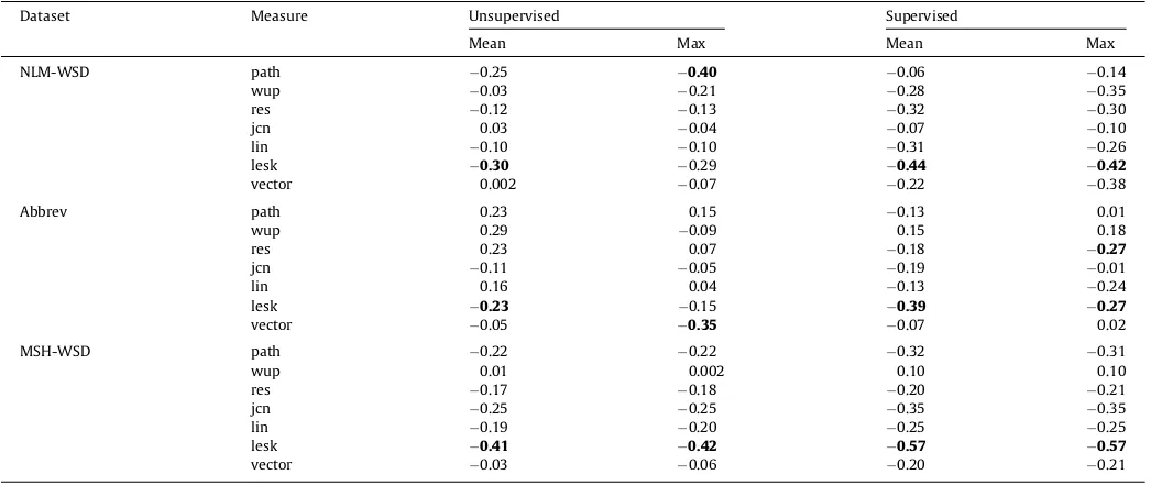
[image:8.595.42.565.86.307.2]5.3.1. Results by data set
Table 7shows the break down of the correlation scores on the NLM-WSD, Abbrev and MSH-WSD datasets individually. The stron-gest negative correlation is produced by theleskmeasure in the majority of cases. For example, usingleskwith the mean similarity measure results in a correlation of0.57 for MSH-WSD and0.44 for NLM-WSD. The picture is more mixed for the Abbrev data set where several of the correlation co-efficients are close to 0. This suggests that the measures are more useful for determining the WSD difficulty of terms than abbreviations.
Further analysis of how well the methods perform on terms and abbreviations was carried out on the MSH-WSD dataset. This data-set contains 203 target words where 106 are terms, 88 are abbre-viations, and 9 have possible senses that are terms and abbreviations.Table 8show the correlation results for each type of ambiguity in this data set. The supervised results show that there is little difference in the correlation results for abbreviations and terms. This indicates that it is able to determine the difficulty
of disambiguating a target word regardless if it is a term or an abbreviation.
The unsupervised results show that it was unable to determine the difficulty of the terms in this dataset which is contrary to what was seen in the Abbrev results fromTable 7. We believe the results from MSH-WSD may provide a more accurate indication on how well the unsupervised method works for two main reasons. The first is that the number of ambiguous abbreviations in the Abbrev dataset is low (16 abbreviations) compared with the MSH-WSD dataset (88 abbreviations). The second is that the disambiguation accuracies of abbreviations in the Abbrev dataset is smaller than those in the MSH-WSD dataset. The accuracies range from 0.96– 1.00 in the Abbrev dataset to 0.89–1.00 in the MSH-WSD dataset.
6. Conclusion and future work
The accuracy of WSD systems for biomedical documents varies enormously across ambiguous terms. It would be useful to be able to predict the difficulty of a particular term for WSD systems in or-der to determine whether applying WSD would be useful. In this paper, we explore a range of approaches to estimating WSD diffi-culty. Some of these are based on information extracted from sense-labeled corpora while others make use of information from knowledge sources. Evaluation was carried out by comparing the predictions made by these measures with the actual accuracy of two different WSD systems on three data sets.
Results show that the supervised methods are good predictors of WSD difficulty in some cases, but that their results are not con-sistent across different data sets. These methods also require la-beled training data, limiting their usefulness. The unsupervised approaches do not have this limitation and can be applied to a
Table 7
Breakdown of spearman’s rank correlation results on the datasets.
Dataset Measure Unsupervised Supervised
Mean Max Mean Max
NLM-WSD path 0.25 0.40 0.06 0.14
wup 0.03 0.21 0.28 0.35
res 0.12 0.13 0.32 0.30
jcn 0.03 0.04 0.07 0.10
lin 0.10 0.10 0.31 0.26
lesk 0.30 0.29 0.44 0.42
vector 0.002 0.07 0.22 0.38
Abbrev path 0.23 0.15 0.13 0.01
wup 0.29 0.09 0.15 0.18
res 0.23 0.07 0.18 0.27
jcn 0.11 0.05 0.19 0.01
lin 0.16 0.04 0.13 0.24
lesk 0.23 0.15 0.39 0.27
vector 0.05 0.35 0.07 0.02
MSH-WSD path 0.22 0.22 0.32 0.31
wup 0.01 0.002 0.10 0.10
res 0.17 0.18 0.20 0.21
jcn 0.25 0.25 0.35 0.35
lin 0.19 0.20 0.25 0.25
lesk 0.41 0.42 0.57 0.57
[image:8.595.312.563.350.408.2]vector 0.03 0.06 0.20 0.21
Table 8
Breakdown of Spearman’s Rank Correlation on MSH-WSD usinglesk. Unsupervised Supervised
MSH-WSD Mean Max Mean Max
Abbreviations 0.26 0.30 0.32 0.35
Terms 0.02 0.01 0.30 0.31
wider range of ambiguities. Our experiments showed that these approaches were also good predictors of WSD difficulty. The best performance was obtained using the relatedness measure pro-posed by Lesk[25]and aggregating the scores using the mean sim-ilarity metric. This method obtained a statistically significantly higher negative correlation than the other measures when com-pared to both the supervised and unsupervised WSD systems (p60.05). The performance of this measure was also reasonably
consistent across different data sets and types of ambiguity (terms and abbreviations). The methods explored in this paper are useful tools for estimating the performance of a WSD system that can be computed without the need for labeled data.
In the future, we plan to explore other relatedness measures that use contextual information about the senses rather than (or in conjunction with) their placement within a taxonomy. We would also like to explore semantic groups of the terms to deter-mine if some types are easier to disambiguate than others.
Acknowledgment
Stevenson is grateful to the UK Engineering and Physical Sciences Research Council for supporting this work (Grant EP/ J008427/1).
References
[1]Liu H, Teller V, Friedman C. A multi-aspect comparison study of supervised word sense disambiguation. J Am Med Infor Assoc 2004;11(4):320–31. [2] Joshi M, Pedersen T, Maclin R, A comparative study of support vector machines
applied to the word sense disambiguation problem for the medical domain. In: Proceedings of the second Indian Conference on Artificial Intelligence (IICAI-05). Pune, India; 2005. p. 3449–68.
[3]Humphrey S, Rogers W, Kilicoglu H, Demner-Fushman D, Rindflesch T. Word sense disambiguation by selecting the best semantic type based on journal descriptor indexing: preliminary experiment. J Am Soc Infor Sci Technol 2006;57(5):96–113.
[4] McInnes B, Pedersen T, Carlis J. Using UMLS Concept Unique Identifiers (CUIs) for word sense disambiguation in the biomedical domain. In: Proceedings of the annual symposium of the american medical informatics association. Chicago, IL; 2007. p. 533–37.
[5] Stevenson M, Guo Y, Gaizauskas R, Martinez D. Disambiguation of biomedical text using diverse sources of information. BMC Bioinformatics 2008;9(Suppl. 11):S7. <http://www.biomedcentral.com/1471-2105/9/S11/S7>.
[6]Agirre E, Sora A, Stevenson M. Graph-based word sense disambiguation of biomedical documents. Bioinformatics 2010;26(2):2889–96.
[7] Jimeno-Yates A, Aronson A. Knolwedge-based biomedical word sense disambiguation: comparison of approaches. BMC Bioinformatics 11(569). [8] Plaza L, Jimeno-Yepes A, Diaz A, Aronson A. Studying the correlation between
different word sense disambiguation methods and summarization effectiveness in biomedical texts. BMC Bioinformatics 2011;12(1):355.
http://dx.doi.org/10.1186/1471-2105-12-355. <http://www.biomedcentral. com/1471-2105/12/355>.
[9] Sanderson M. Word sense disambiguation and information retrieval. In: Proceedings of the 17th ACM SIGIR conference. Dublin, Ireland; 1994. p. 142– 51.
[10]Weeber M, Klein H, Berg L, Vos R. Using concepts in literature-based discovery. JASIST 2001;57(7):548–57.
[11]Swanson D. Migraine and magnesium – 11 neglected connections. Perspect Biol Med 1988;31(4):526–57.
[12] Stevenson M, Guo Y, Alamri A, Gaizauskas R. Disambiguation of biomedical abbreviations. In: Proceedings of the BioNLP 2009 workshop, association for computational linguistics. Boulder, Colorado; 2009. p. 71–9. <http:// www.aclweb.org/anthology/W/W09/W09-1309>.
[13]Artstein R, Poesio M. Inter-coder agreement for computational linguistics. Comput Linguist 2008;34(4):555–96.
[14]Jimen-Yepes A, McInnes B, Aronson A. Exploiting MeSH indexing in MEDLINE to generate a data set for word sense disambiguation. BMC Bioinformatics 2011;12(1):223.
[15]Humphreys L, Lindberg D, Schoolman H, Barnett G. The unified medical
language system: an informatics research collaboration. J Am Med Infor Assoc 1998;1(5):1–11.
[16]Ide N, Loane R, Demner-Fushman D. Essie: a concept-based search engine for structured biomedical text. J Am Med Infor Assoc 2007;14(3):253–63.
[17]Nelson S, Powell T, Humphreys B. The unified medical language system
(UMLS) project. Encyclopedia Lib Infor Sci 2002:369–78.
[18]Rada R, Mili H, Bicknell E, Blettner M. Development and application of a metric on semantic nets. IEEE Trans Syst Man Cyber 1989;19(1):17–30.
[19]Caviedes J, Cimino J. Towards the development of a conceptual distance metric for the UMLS. J Biomed Infor 2004;37(2):77–85.
[20] Wu Z, Palmer M. Verbs semantics and lexical selection. In: Proceedings of the 32nd meeting of association of computational linguistics. Las Cruces, NM; 1994. p. 133–38.
[21]Cover T, Thomas J. Elements of information theory. New York: Wiley;
1991.
[22] Resnik P. Using information content to evaluate semantic similarity in a taxonomy. In: Proceedings of the 14th international joint conference on artificial intelligence. Montreal, Canada; 1995. p. 448–53.
[23] Jiang J, Conrath D. Semantic similarity based on corpus statistics and lexical taxonomy. In: Proceedings on international conference on research in computational linguistics. Tapei, Taiwan; 1997. p. 19–33.
[24] Lin D. An information-theoretic definition of similarity. In: Intl Conf ML Proc. San Francisco, CA; 1998. p. 296–304. <citeseer.ist.psu.edu/95071.html>. [25] Lesk M. Automatic sense disambiguation using machine readable dictionaries:
how to tell a pine cone from an ice cream cone. In: Proceedings of the 5th annual international conference on systems documentation. Toronto, Canada; 1986. p. 24–6.
[26] Banerjee S, Pedersen T. Extended gloss overlaps as a measure of semantic relatedness. In: Proceedings of the eighteenth international joint conference on artificial intelligence. Acapulco, Mexico; 2003. p. 805–10.
[27] Patwardhan S, Pedersen T. Using WordNet-based context vectors to estimate the semantic relatedness of concepts. In: Proceedings of the EACL 2006 workshop making sense of sense – bringing computational linguistics and psycholinguistics together. Trento, Italy; 2006. p. 1–8.
[28]Kilgarriff A, Rosenzweig J. Framework and results for English SENSEVAL. Comput Humanities 2000;34(1-2):15–48.
[29] Kilgariff A, Palmer M, editors. Proceedings of the Pilot SensEval, association for computational linguistics. Hermonceux Castle, Sussex, UK; 1998. <http:// www.aclweb.org/anthology/S98-1>.
[30] McCarthy D, Koeling R, Weeds J, Carroll J. Finding predominant word senses in untagged text. In: Proceedings of the 42nd Meeting of the Association for Computational Linguistics (ACL’04), main volume. Barcelona, Spain; 2004. p. 279–86. doi:10.3115/1218955.1218991. <http://www.aclweb.org/anthology/ P04-1036>.
[31] Jin P, McCarthy D, Koeling R, Carroll J. Estimating and exploiting the entropy of sense distributions. In: Proceedings of human language technologies: the 2009 annual conference of the North American chapter of the association for computational linguistics, companion volume: short papers. Association for Computational Linguistics, Boulder, Colorado; 2009. p. 233–36. <http:// www.aclweb.org/anthology/N/N09/N09-2059>.
[32] Agirre E, Edmonds PG, editors. Word sense disambiguation: algorithms and applications. Springer; 2006.
[33] Stevenson M, Guo Y. The effect of ambiguity on the automated acquisition of wsd examples. In: Human language technologies: the 2010 annual conference of the North American chapter of the association for computational linguistics. Association for Computational Linguistics, Los Angeles, California; 2010. p. 353–56. <http://www.aclweb.org/anthology/N10-1053>.
[34]Palmer M, Dang HT, Fellbaum C. Making fine-grained and coarse-grained sense distinctions, both manually and automatically. Nat Language Eng 2007;13(2): 137.
[35] McInnes B, Pedersen T, Pakhomov S. UMLS-interface and UMLS-similarity: open source software for measuring paths and semantic similarity. In: Proceedings of the American Medical Informatics Association (AMIA) symposium. San Fransico, CA; 2009.
[36]Stevenson M, Guo Y, Gaizauskas R, Martinez D. Disambiguation of biomedical text using diverse sources of information. BMC Bioinformatics 2008;9(Suppl. 11):11.
[37] McInnes B, Pedersen T, Liu Y, Pakhomov S, Melton G. Using second-order vectors in a knowledge-based method for acronym disambiguation. In: Proceedings of the conference on computational natural language learning. Portland, OR; 2011.
[38] Agirre E, Martinez D. The basque country university system: english and basque tasks. In: Proceedings of the 3rd ACL workshop on the evaluation of systems for the semantic analysis of text (SENSEVAL-3) at the annual meeting of the association of computational linguistics. Barcelona, Spain; 2004. p. 44–8.
[39] Stevenson M, Guo Y, Al Amri A, Gaizauskas R. Disambiguation of biomedical abbreviations. In: Proceedings of the ACL BioNLP workshop; 2009. p. 71–9.
[40]Liu H, Lussier Y, Friedman C. Disambiguating ambiguous biomedical terms in biomedical narrative text: an unsupervised method. J Biomed Infor 2001; 34(4):249–61.
[41] Weeber M, Mork J, Aronson A. Developing a test collection for biomedical word sense disambiguation. In: Proceedings of AMIA Symposium. Washington, DC; 2001. p. 746–50.