White Rose Research Online
[email protected]
Universities of Leeds, Sheffield and York
http://eprints.whiterose.ac.uk/
This is the author’s post-print version of an article published in the
IEEE
Photonics Journal
White Rose Research Online URL for this paper:
http://eprints.whiterose.ac.uk/id/eprint/78212
Published article:
Tych, KM, Wood, CD and Tych, W (2014)
A simple transfer-function-based
approach for estimating material parameters from terahertz time-domain data.
IEEE Photonics Journal, 6 (1). 6671984. ISSN 1943-0655
A Simple Transfer-Function-Based Approach for
Estimating Material Parameters from Terahertz
Time-Domain Data
K. M. Tych , C. D. Wood and W. Tych
School of Physics and Astronomy, University of Leeds, School of Electronic and Electrical Engineering, University of Leeds and Lancaster Environment Centre, Lancaster University,
United Kingdom
DOI: 10.1109/JPHOT.2011.XXXXXXX 1943-0655/$25.00 c2011 IEEE
Abstract: A novel parametrically efficient approach to estimating the spectra of short transient
signals is proposed and evaluated, with an application to estimating material properties, including complex refractive index and absorption coefficient, in the terahertz (THz) frequency range. This technique includes uncertainty analysis of the obtained spectral estimates, allowing rigorous statistical comparison between samples. In the proposed approach, a simple, few-parameter continuous-time transfer function model explains over 99.9% of the measured signal. The problem, normally solved using poorly numerically defined Fourier transform deconvolution methods, is reformulated and cast as a time-domain dynamic-system estimation problem, thus providing a true time-domain spectroscopy tool.
Index Terms: Terahertz, terahertz sensing, novel methods, modeling
1. Introduction
The terahertz (THz) frequency range is commonly defined to lie between 0.3 and 10 THz, and corresponds to a range of fundamental material properties including: low frequency chemical bond vibrations, crystalline phonon vibrations, hydrogen-bond stretches and torsion motions [1]. THz time-domain spectroscopy (THz-TDS) is becoming an established technique for substance identification and for obtaining material parameters in the form of the refractive index and ab-sorption coefficient spectra of a broad range of samples, including small molecules [2], [3], [4], biological samples [5], [6], and semiconductors [7], [8]. THz-time domain data often takes the form of a single pulse, less than a picosecond in duration, followed by a series of attenuated pulses arising either from reflections at the interface of components within the TDS system, or from etalon reflections within the sample itself. Typically, two separate measurements are taken: one serves as a reference and consists of a free-space, or empty sample cell measurement, and the second comprises what is normally assumed to be a convolution of the reference and the sample itself, often referred to as the ’cross spectrum’ when considering the frequency domain interpretation. To extract spectral estimates purporting to the sample alone, the reference signal must, therefore, be deconvolved from the second signal.
In terahertz time-domain spectroscopy, the PSD of finite time-domain THz pulses are commonly estimated using the Fast Fourier Transform (FFT) or some variation [2]. Fourier Transforms operate on the principle that the measured signal, which has been recorded for a finite time period, is repeated indefinitely outside that time window. Whilst the Fourier transform is therefore suited to the frequency analysis of periodic signals, a pulsed (transient) signal is likely to end at a discontinuity which the FFT will then include in the transform. Sharp discontinuities in the time-domain contain a broad frequency spectrum, and will therefore cause the signal’s frequency spectrum to be spread out (spectral leakage). Furthermore, any given frequency in the output spectrum will contain energy both from the signal and from noise arising from the rest of the spectrum. The raw periodogram produced by the Fourier Transform is therefore considered a poor spectral estimate, as its variance at a given frequency does not decrease with the number of samples used to perform the transfer function, and is indeed equal to the square of its expectation value [9]. Variance and spectral leakage may be reduced by, respectively, smoothing of the signal and windowing of the time-series - which effectively multiplies the finite time domain signal with a periodic envelope. The resultant convolution is then Fourier transformed. The choice of the smoothing and window functions introduces a trade-off between the resulting spectral resolution (i.e. the ability to distinguish closely-spaced features), and how efficiently the spectral leakage is reduced [10]. These choices, which rely heavily on the interpretation of the user, can therefore affect significantly the resulting PSD resolution, bias and variance, leading to differences in the positions and intensities of absorptions / resonances in the frequency domain, potentially even obscuring weaker features which are in close proximity to stronger signals [11].
The method of deconvolving the data, i.e. dividing the cross-spectrum by the reference spectrum to obtain the sample spectrum, carries with it two strong assumptions. The first is the treatment of both objects as dynamic Linear Time Invariant (LTI) systems, namely that the system is fully characterized by its amplitude and phase responses (Linear), and that these amplitude and phase responses do not change in time (Time Invariant). The second assumption is that both spectral estimates are good in terms of their bias and inherent uncertainty. Duvillaret et al. address this by presenting a method of calculating physical sample characteristics from their spectral response, including estimates of the associated uncertainty [12]. Separately, Dorney et al., and later Pupeza
et al. describe methods for improving the accuracy of material parameter estimation from
time-domain signals, indicating the need for regularization of the poorly defined deconvolution process and the numerical problems encountered [13], [14].
In this paper, we suggest that a more accurate and robust approach would be to avoid de-convolution in the frequency domain - and its associated uncertainties - altogether, and instead, at the estimation stage, to deal only with the time-domain data (thus remaining true to the term ‘Time Domain Spectroscopy’). We demonstrate that, by treating the spectral response in the time domain as a dynamic system’s impulse response with transient components, it is possible to reliably and easily obtain accurate frequency domain characteristics, directly comparable to those published in the literature, without the need and therefore without the associated error -for windowing or padding of the recorded data. Additional in-formation, in the -form of uncertainty bounds, provides objective measures of quality of spectrum and thus has the potential to improve substance identification, for example, in THz spectroscopy.
2. Methods
2.1. ExperimentThe time-domain data was collected using the broadband THz-TDS system at the Institute of Microwaves and Photonics, University of Leeds, described in detail elsewhere [2]. Pressed-pellet samples of two materials well-characterised in the THz-frequency range were chosen for study:
of five time-domain measurements taken from different points on the pellet samples were used for analysis, to minimise error arising from imperfect mixing and sample-thickness measurements. Both the reference THz signal, and that after transmission through the sample, were collected and focused onto an electro-optic crystal, enabling electro-optic (EO) sampling of the THz radiation in the time domain.
The EO crystal is only birefringent for the time that the THz field is present. This makes it possible to reconstruct a complete time domain signal from independent measurements of adjacent portions of a train of (ideally) identical THz pulses. In order to improve accuracy, and to reduce the noise in the spectrum, signal averaging was used. The acquisition time for each time domain spectrum is therefore limited by both the number of single measurements and the minimum time limit to any sampling technique (tmin≥N·δt) whereN is the number of data points required to measure the whole THz pulse, andδtis the pulse spacing in the pulse train [25].
In order for the time-domain data to be Fourier transformed into the frequency domain, it must first be truncated before the reflection peak arising from the EO crystal (∼4.7 ps after the main signal) to remove spurious oscillations from the frequency spectrum [2]. The peak originates from etalon reflections within the EO crystal, and therefore its position is determined by the crystal thickness. This truncation reduces the amount of data used in the FFT calculation, thus limiting the number of discrete data points in the resulting frequency spectrum. A typical, truncated data set may consist of, for example, 600 data points which, for an efficient FFT, is often truncated or padded to the next power of 2 (i.e. 512, or 1024). The effect of zero padding is to interpolate between actual data points in the frequency spectra and often produces a smoother response. Additional padding (to subsequent powers of 2) may be undertaken at the user’s discretion to increase further the number of data points in the frequency spectra though this does not overcome the spectral resolution limitations inherent to the measurement and analysis, and may therefore mislead a user into believing that all spectral features have been resolved. Furthermore, care must be taken to avoid padding-artifacts by the introduction of sharp discontinuities. Following FFT, the resultant data may then be used to extract the frequency dependent absorption coefficient and complex refractive index, using a combination of Fresnel equations and the Beer-Lambert law, described in detail in the supplementary information.
2.2. Proposed analysis technique
Transfer functions utilizing physics-based estimations (e.g. Equation 1) have been used previously to estimate physical characteristics of materials probed using THz radiation. Such functions relay directly the effect on the input THz signal,Esam(ω)of the material’s complex refractive index,nˆ(ω), extinction coefficient, κ(ω) and sample thickness, l, which result in the observed output signal,
E(ω)[24].
Esam(ω)
Erefω
= 4ˆn(ω)n0 [ˆ(n)(ω) +n0]2
exp
−κ(ω)ωl
x
exp
−j[n(ω)−n0]
ωl c
(1)
However, such physical transfer functions remain difficult to solve, and often require the introduc-tion of approximaintroduc-tions to simplify the calculaintroduc-tions, thereby introducing a further source of error. An alternative approach is to use a data-based rational polynomial spectral estimation. The technique of obtaining frequency domain spectra from temporal waveforms using parametric spectral estima-tion is well established (see e.g. [26] and [9]). Some methods include: univariate auto-regressive (AR)-based [27], [28] and auto-regressive moving average (ARMA)-based spectral estimates, and related cross-spectral estimates based on Laplace transfer functions [9]. A univariate approach is logical where there is no knowledge of the character or timing of the input signal. In this case, however, we are interested in cross-spectrum estimation, as we wish to deconvolve the spectral response of the sample from the sample and free space cross-spectrum and a transfer function estimation is therefore more appropriate.
the Laplace domain and are direct, complex rational approximations of cross-spectra [9]. When a good model fit is obtained (i.e. one which explains over 99% of the output data variance) using a transfer function with a given number of parameters, it means that any further detail obtained by increasing the number of parameters is quite likely to consist primarily of noise and artifacts. It is worth noting at this point that for the data we analyzed, simple 12thorder and 18thorder transfer function models with only 24 and 36 parameters, respectively, explained 99.98% of the output variance of the measured samples. This implies that even a smoothed Fourier spectrum would be “over-parameterised”, estimating, for example, an equivalent of 1024 values from the same sample of 600 points. A further advantage of using this technique is that the 20+ parameters in the transfer function, can be used directly to numerically estimate vibrational and relaxational processes within the sample (seen as dynamic modes observable in the time domain data) in response to the THz pulse, effectively enabling the reverse-engineering of the dominant dynamic modes of the sample [29].
Most of the methods in the references cited are based on discrete-time transfer functions. The main disadvantage of discrete-time models is that they only work well for a narrow spectral range: limited by Popov’s Theorem at the high end of the spectrum, and by the numerical problems of esti-mating oversampled, discrete systems at the low end. The low frequencies are compressed owing to mapping between the left, complex half-plane of the continuous system’s poles (eigenvalues) and the unit circle of the discrete system’s poles. This causes problems with effective estimation of systems with broad spectra. The alternative continuous-time form of transfer functions has gained popularity in recent years owing to the development of modern estimation methods for continuous time systems [30], [31], [32], [33]. Continuous-time models, as used in this work, can be used for systems with a broad spectral range, and allow precise spectral estimation at the low-frequency end of the useful spectrum.
The transfer function, which is a data-based analogue of Equation 1, is estimated directly in the following form, using the continuous Laplace operatorsof orderm, n(wheremis the order of the numerator and n the denominator), with a time delay τ between the reference and transmitted time-domain signals:
Y(s) =P(s)
Q(s) =
β0sm+β1sm− 1
+· · ·+βm
sn+α
1sn−1+· · ·+αn
e−sτU(s) (2)
where U(s) = L{u(t)} and Y(s) = L{y(t)} are, assuming zero initial conditions, the Laplace transforms of the system’s respective input (in this case, the reference THz signal) and output (the THz pulse transmitted through the material under test).The spectrum is then calculated by substitutings=j2πν, whereν is the normalized frequency.
The problem remains of effective estimation of transfer function models which will not produce spurious spectral peaks (caused for instance by estimating dynamic modes not sufficiently rep-resented in the data), but which, at the same time, will explain the data sufficiently well. This is addressed by identifying parametrically efficient structures from a range of transfer function models fitted to the input-output data set (i.e. data-based mechanistic methodology [34], [29]).
uncertainty in the calculated material parameters. This provides a vital tool when comparing the characteristics of different substances or samples, by allowing rigorous statistical comparisons between different measurements.
For each signal series, the proposed procedure consists of:
1) Forming a pair of input-output signals by selecting a meaningful temporal range of the measured reference spectrum and cross-spectrum time-domain signals (i.e. truncating the data before the first reflection peak, as described in the supplementary information). 2) Identifying the structure of a continuous-time transfer function. This is achieved by assessing
the suitability of a wide range of models, each of which has the form:
b
Y(s) = Pb(s)
b
Q(s)U(s) =
c
β0sm+cβ1sm− 1
+· · ·+βcm
sn+αc
1sn−1+· · ·+αcn
e−sτU(s) (3)
with different ordersmandn, and time delays,τ. This transfer function is a rational, complex data-based analogue of Equation 1, and allows estimation of the effect of the material on the THz signal. The final model selection uses an Information-based Criterion (IC), similar to Akaike’s (AIC) [28], [29], which allows the selection of a parametrically efficient representation of the time-domain signal, by varyingm,n, andτ, whilst maintaining a good fit based on a highR2
t value:
R2t = 1−
σ2 e
σ2 y
(4)
σ2
e is the variance of model residuals e(t) = y(t)−Yˆ(t), and σ 2
y is the variance of the
observed output variabley.
3) Estimating the coefficients of the selected transfer function, and calculating the associated spectrum. The transfer function is estimated using the continuous-time Simplified Refined In-strumental Variable (SRIV) method [30]. The SRIV method is related to linear, least squares algorithms, but is designed specifically for continuous-time dynamic systems, and is im-plemented in the CAPTAIN Toolbox for Matlab [33]. This yields the estimated coefficients
ˆ
β0. . .βˆm,αˆ1. . .αˆn in Equation 3. The complex-conjugate pairs of roots of the transfer
func-tion denominator determine the frequencies and damping of the dominant oscillatory modes of the material. The complex spectrum estimate is then calculated simply by substituting
s=j2πν into the expression forGb(s)in Equation. 3. The material characteristics (refractive index and absorption coefficient) as functions of frequencyν, are then calculated from the obtained complex spectrum estimate, using the same method as for FFT-based calculations (see Supplementary Information).
matrix of these parameters as obtained from the same SRIV procedure. Each of these parametric realisations is then used to calculate a realisation of the physical characteristics of the sample, thus providing distributions of these characteristics at each frequency.
It should be noted that the transfer function estimate used to calculate the spectrum is obtained directly from the pair of time-domain signals (sample and reference), with no additional data (e.g. in the form of padding), or assumptions (e.g. windowing), other than the choice of truncation time (Step (1), above). Steps (2) - (4) are easily automated in a MatlabTM script, an example of which can be obtained from the authors. Steps (3) and (4) take a few seconds to complete. However, initial identification of a suitable model order for each sample measured (Step (2)) is likely to take longer owing to the need to evaluate high numbers of potential models of different orders. The technique will be continually refined in future work, and the prospect of real-time data analysis in later iterations is therefore not precluded.
The technique presented here provides a reliable and well defined estimate of sample spectrum along with its uncertainty, as well as a secondary estimate of the refractive index and absorption coefficient, assuming a known sample thickness. In the case of an unknown sample thickness, a procedure for extraction of material parameters can be applied, where the thickness and refractive index are obtained using Fabry-P ´erot oscillations from the frequency domain (which originate from etalon reflections within the sample) analogous to the Quasi-space [35] or Total Variation methods [14]. Unlike these techniques however, because of the lower uncertainty of the spectral estimate itself, the frequency domain material characteristics extracted using the method proposed here, will have significantly lower numerical uncertainty resulting in more accurate estimates.
3. Results
0 1 2 3 4 5 6
Time (ps) -80
-60 -40 -20 0 20 40
Amplitude (a.u.)
60 Reference (free space)
[image:7.594.196.435.364.548.2]Sample (lactose monohydrate)
Fig. 1. Truncated THz time-domain measurements of the empty-frame-plus-free-space reference signal (dashed line), and the resultant pulse after transmission through a pressed pellet of 12.5 % lactose (solid line) in a PTFE matrix, showing both the time-delay and reduction in amplitude of the transmitted THz pulse following interaction with the sample.
0 1 2 3 4 5 6 -30
-20 -10 0 10 20 30
Time (ps)
0.0 0.5 1.0 1.5 2.0 2.5 3.0 3.5 4.0
-30 -20 -10 0 10 20 30
Time (ps)
Model fit Experimental data (a) (b)
Amplitude (a.u.) Amplitude (a.u.)
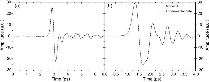
Fig. 2. (a) Lactose time-domain TF (transfer function) model fit and (b) glucose time-domain TF model fit. 95% uncertainty bands, obtained from the transfer function estimation, are shown as gray bands in both figures, though they are too narrow to resolve from the TF estimates.
The time-domain signals for each sample can be reconstructed using relatively low-order trans-fer function models; 18th order for lactose (Fig.2(a)), and12th order for glucose (Fig.2(a)). Both
models are found to explain almost 99.99% of the output variance for the data sets analyzed. As over-parametrisation can lead to (a) spurious dynamic modes and spectral peaks, and (b) poor definition (higher uncertainty) of the estimated parameters, the model orders are selected using a combination of model fitting and low-order parametrisation. The fit is measured using an R2
t criterion (Equation 4), obtained by running the input series through the transfer function
model and comparing it with the observed output. The calculated R2
t typically lay between 0.99
and 0.999 (where 1.00 represents a 100% fit), indicating that all practically useful information has been encapsulated by the transfer function. This in turn implies that using spectral estimation techniques with more complicated parametrization, such as FFT based methods, will not produce a significantly better fit, and will more likely result in increased error and poorly defined results.
The material parameter uncertainty estimates, derived from the transfer function parameters and their covariance matrices as percentile based uncertainty bounds, are shown as grey bands in Fig.2(a) and Fig.2(b)). The absolute error values are affected by a combination of the sample and experimental characteristics, including the subjective choice of data truncation point. It can be seen that the uncertainty for both samples is small (indeed they are hidden immediately behind the TF representation of the time-domain data) indicating a good model fit.
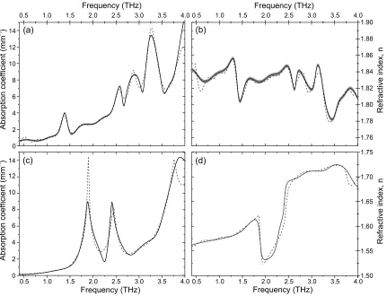
For comparison with FFT techniques, frequency-domain estimates were calculated by substi-tution of s = j2πν into Equation 3, for both the reference and sample measurements for each material. These were next analyzed as described in the supplementary information, using Fresnel equations and the Beer-Lambert law. Fig.3(a) and Fig.3(b) show, respectively, the frequency-dependent absorption coefficient and refractive index, obtained between 0.4 – 4 THz for the lactose pellet. Equivalent results between 0.4 – 4 THz obtained from a pressed powder pellet containing 100% glucose are shown in Fig.3(c) and Fig.3(d). In each plot, FFT data are shown as dashed lines, and solid lines represent the Transfer Function estimates.
[image:8.594.98.527.68.237.2]0 2 4 6 8 10 12 14
1.76 1.78 1.80 1.82 1.84 1.86 1.88 1.90
0 2 4 6 8 10 12 14
1.50 1.55 1.60 1.65 1.70 1.75
Absorption coef
ficient (mm
)
-1
Absorption coef
ficient (mm
)
-1
Refractive index, n
Refractive index, n
0.5 1.0 1.5 2.0 2.5 3.0 3.5 4.0
Frequency (THz)
0.5 1.0 1.5 2.0 2.5 3.0 3.5 4.0
Frequency (THz)
4.0 0.5 1.0 1.5 2.0 2.5 3.0 3.5
Frequency (THz)
(a)
0.5 1.0 1.5 2.0 2.5 3.0 3.5 4.0
(b)
Frequency (THz)
[image:9.594.101.532.63.393.2](c) (d)
Fig. 3. Absorption coefficient and refractive index estimates showing the TF with 95% uncertainty band (solid line, uncertainty band shaded grey) and for the FFT-based approach (dotted line) for (a), (b) 12.5 % lactose sample and (c), (d) the 100% glucose sample. As for the time-domain estimates, the error band associated with the glucose sample is very narrow and lies directly beneath the calculated sample characteristics in (c) and (d).
parameters: one obtained using a standard FFT of the time-domain data, and one from data extracted using the proposed continuous-time transfer function. While similarities between the extracted parameters provides some degree of confidence in the proposed technique, perfect agreement is neither required nor expected. The frequency positions of the absorption peaks in the lactose sample are in good agreement with those published in the literature [23], [36].
4. Conclusions
Data and software availability
Both data and Matlab scripts used to prepare this Open Access publication can be obtained from the corresponding author. The CAPTAIN Toolbox for Matlab can be obtained from the URL below or by contacting the corresponding author. ( http://www.es.lancs.ac.uk/cres/captain/ )
Acknowledgements
The authors wish to thank Lancaster University for providing funding for this Open Access pub-lication. The data was collected using the broad bandwidth THz-TDS system in the School of Electronic and Electrical Engineering at the University of Leeds, UK. The authors wish to thank Dr. A. D. Burnett for help with data collection and Professors A. G. Davies, E. H. Linfield and J. E. Cunningham for providing access to the laboratory where the THz data was obtained. The authors also wish to express their thanks to the anonymous reviewers who contributed their time and provided extremely useful critical comments, which served to improve the paper.
References
[1] C. J. Strachan, P. F. Taday, D. Newnham, K. Gordon, J. Zeitler, M. Pepper, and T. Rades, “Using terahertz pulsed spectroscopy to quantify pharmaceutical polymorphism and crystallinity,” J. Pharm. Sci., vol. 94, no. 4, pp. 837 – 846, 2005.
[2] W. H. Fan, A. Burnett, P. C. Upadhya, J. Cunningham, E. H. Linfield, and A. G. Davies, “Far-Infrared Spectroscopic Characterization of Explosives for Security Applications Using Broadband Terahertz Time-Domain Spectroscopy,”
Appl. Spectrosc., vol. 61, no. 6, pp. 638–643, Jun. 2007.
[3] Y. C. Shen, T. Lo, P. Taday, B. Cole, W. Tribe, and M. Kemp, “Detection and identification of explosives using terahertz pulsed spectroscopic imaging,” Appl. Phys. Lett., vol. 86, no. 24, p. 241116, 2005.
[4] B. Fischer, M. Hoffmann, H. Helm, G. Modjesch, and P. Uhd Jepsen, “Chemical recognition in terahertz time-domain spectroscopy and imaging,” Semicond. Sci. Technol., vol. 20, no. 7, pp. S246–S253, 2005.
[5] K. Tych, A. Burnett, C. Wood, J. Cunningham, A. Pearson, A. Davies, and E. Linfield, “Applying broadband terahertz time-domain spectroscopy to the analysis of crystalline proteins: a dehydration study,” J. Appl. Crystallogr., vol. 44, no. 1, pp. 129–133, Feb. 2011.
[6] A. Markelz, A. Roitberg, and E. Heilweil, “Pulsed terahertz spectroscopy of DNA, bovine serum albumin and collagen between 0.1 and 2.0 THz,” Chem. Phys. Lett., vol. 320, no. 1–2, pp. 42–48, 2000.
[7] D. Grischkowsky, S. Keiding, M. van Exter, and C. Fattinger, “Far-infrared time-domain spectroscopy with terahertz beams of dielectrics and semiconductors,” J. Opt. Soc. Amer. B, vol. 7, no. 10, pp. 2006–2015, 1990.
[8] T.-I. Jeon and D. Grischkowsky, “Characterization of optically dense, doped semiconductors by reflection THz time-domain spectroscopy,” Appl. Phys. Lett., vol. 72, no. 23, pp. 3032–3034, 1998.
[9] P. Stoica and R. Moses, Introduction to Spectral Analysis, 2nd ed. Prentice-Hall, 1997.
[10] J. M. Spyers, P. G. Bain, and S. J. Roberts, “A comparison of fast fourier transform (FFT) and autoregressive (AR) spectral estimation techniques for the analysis of tremor data,” J. Neurosci. Meth., vol. 83, no. 1998, pp. 35–43, 1998. [11] K. Aki and P. Richards, Quantitative Seismology. W.H. Freeman and Co., 1980.
[12] L. Duvillaret, F. Garet, and J.-L. Coutaz, “Influence of noise on the characterization of materials by terahertz time-domain spectroscopy,” J. Opt. Soc. Amer., vol. 17, no. 3, pp. 452–461, Mar 2000.
[13] T. D. Dorney, R. G. Baraniuk, and D. M. Mittleman, “Material parameter estimation with terahertz time-domain spectroscopy,” J. Opt. Soc. Amer. A, vol. 18, no. 7, pp. 1562–1571, 2001.
[14] I. Pupeza, R. Wilk, and M. Koch, “Highly accurate optical material parameter determination with THz time-domain spectroscopy,” Opt. Exp., vol. 15, no. 7, pp. 4335–4350, Apr 2007.
[15] E. R. Brown, J. E. Bjarnason, A. M. Fedor, and T. M. Korter, “On the strong and narrow absorption signature in lactose at 0.53THz”,” Applied Physics Letters, vol. 90, no. 6, p. 061908, 2007.
[16] M. Walther, M. Freeman, and F. A. Hegmann, “Metal-wire terahertz time-domain spectroscopy,” Applied Physics
Letters, vol. 87, no. 26, p. 261107, 2005.
[17] D. Allis, A. Fedor, T. Korter, J. Bjarnason, and E. Brown, “Assignment of the lowest-lying THz absorption signatures in biotin and lactose monohydrate by solid-state density functional theory,” Chemical Physics Letters, vol. 440, no. 4 - 6, pp. 203 – 209, 2007.
[18] H. Tuononen, E. Gornov, J. A. Zeitler, J. Aaltonen, and K.-E. Peiponen, “Using modified kramers–kronig relations to test transmission spectra of porous media in thz-tds,” Opt. Lett., vol. 35, no. 5, pp. 631–633, 2010.
[19] B. Fischer, M. Hoffmann, H. Helm, G. Modjesch, and P. U. Jepsen, “Chemical recognition in terahertz time-domain spectroscopy and imaging,” Semiconductor Science and Technology, vol. 20, no. 7, p. S246, 2005.
[20] X. Li, Z. Hong, J. He, and Y. Chen, “Precisely optical material parameter determination by time domain waveform rebuilding with THz time-domain spectroscopy,” Optics Communications, vol. 283, no. 23, pp. 4701–4706, 2010. [21] Y. Ueno and K. Ajito, “Analytical terahertz spectroscopy,” Analytical Sciences, vol. 24, no. 2, pp. 185–192, 2008. [22] M. B. Byrne, J. Cunningham, K. Tych, A. Burnett, M. Stringer, C. Wood, L. Dazhang, M. Lachab, E. Linfield, and
[23] J. F. Federici, B. Schulkin, F. Huang, D. Gary, R. Barat, F. Oliveira, and D. Zimdars, “THz imaging and sensing for security applications - explosives, weapons and drugs,” Semiconductor Science and Technology, vol. 20, no. 7, p. S266, 2005.
[24] W. Withayachumnankul, B. M. Fischer, H. Lin, and D. Abbott, “Uncertainty in terahertz time-domain spectroscopy measurement,” J. Opt. Soc. Am. B, vol. 25, no. 6, pp. 1059–1072, Jun 2008.
[25] W. Chan, J. Deibel, and D. Mittleman, “Imaging with terahertz radiation,” Rep. Prog. Phys., vol. 70, pp. 1325–1333, 2007.
[26] S. Kay and S. J. Marple, “Spectrum analysis - a modern perspective,” Proc. IEEE, vol. 69 (11), pp. 1380–1419, Nov. 1981.
[27] J. Burg, “Maximum entropy spectral analysis,” in Modern spectrum analysis, D. Childers, Ed. New York: IEEE Press, 1978, pp. 34–41.
[28] H. Akaike, “A new look at the statistical model identification,” IEEE Trans. Automatic Control, vol. AC-19, pp. 716–723, Dec. 1974.
[29] P. Young, “Data-based mechanistic modelling, generalised sensitivity and dominant mode analysis,” Comput. Phys.
Commun., vol. 117, no. 1-2, pp. 113 – 129, Mar. 1999.
[30] P. Young and H. Garnier, “Identification and estimation of continuous-time, data-based mechanistic (DBM) models for environmental systems,” Environ. Modell. Softw., vol. 21, no. 8, pp. 1055 – 1072, Aug. 2006.
[31] P. Young, H. Garnier, and M. Gilson, “Refined instrumental variable identification of continuous-time hybrid box-jenkins models,” in Identification of Continuous-time Models from Sampled Data, ser. Advances in Industrial Control, H. Garnier and L. Wang, Eds. Springer London, 2008, pp. 91–131.
[32] H. Garnier, M. Gilson, T. Bastogne, and M. Mensler, “The contsid toolbox: A software support for data-based continuous-time modelling,” in Identification of Continuous-time Models from Sampled Data, ser. Advances in Industrial Control, H. Garnier and L. Wang, Eds. Springer London, 2008, pp. 249–290.
[33] C. J. Taylor, D. J. Pedregal, P. C. Young, and W. Tych, “Environmental time series analysis and forecasting with the captain toolbox,” Environ. Modell. Softw., vol. 22, no. 6, pp. 797 – 814, Jun. 2007.
[34] P. Young, S. Parkinson, and M. Lees, “Simplicity out of complexity in environmental modelling: Occam’s razor revisited,”
J. Appl. Stat., vol. 23, no. 2-3, pp. 165–210, Jun. 1996.
[35] M. Scheller, C. Jansen, and M. Koch, “Analyzing sub-100-µm samples with transmission terahertz time domain
spectroscopy,” Opt. Commun., vol. 282, no. 7, pp. 1304–1306, Apr. 2009.
[36] W. R. Tribe, D. A. Newnham, P. F. Taday, and M. C. Kemp, “Hidden object detection: security applications of terahertz technology,” Proc. SPIE, vol. 5354, pp. 168–176, 2004.
[37] P. Uhd Jepsen and B. Fischer, “Dynamic range in terahertz time-domain transmission and reflection spectroscopy,”
Opt. Lett., vol. 30, no. 1, pp. 29–31, 2005.
Biographies
K. M. Tych received the degree of BEng(Hons) in Electronic and Electrical Engineering in 2007,
from the University of Leeds. In 2007, she joined the Institute of Microwaves and Photonics at the same University, to study for a PhD entitled ’Terahertz time-domain spectroscopy of biological macromolecules’, working with Professors Giles Davies, Edmund Linfield and John Cunningham, and Dr. Arwen Pearson. On completing her PhD, she joined the Molecular and Nanoscale Physics group at the University of Leeds, working with Dr. Lorna Dougan and Dr. David Brockwell using single-molecule spectroscopic techniques to investigate the mechanical properties of proteins.
C. D. Wood received the degree of BSc(Hons) in Physics with Electronics and Instrumentation
from the University of Leeds, followed by an MSc(Dist) in Nanoscale Science and Technology with the Universities of Leeds and Sheffield. In 2003, he joined the Institute of Microwaves and Photonics at the University of Leeds to study for a PhD in ’On-chip Terahertz Systems’, with Professors Ian Hunter and John Cunningham. Following several PDRA positions, he now holds a University Reseearch Fellowship in ’High Frequency and Mesoscopic Electronics’ at Leeds, in which he uses guided-wave THz devices to probe the ultra-fast properties of mesoscopic systems.
W. Tych received the M.Eng degree in Electronics and Control Engineering in 1979, and the
Supplementary Information
Current data analysis techniqueThe coherent detection of THz pulses in the time domain allows both the frequency-dependent absorption coefficient and refractive index of the sample studied to be calculated from the
atten-uation of the transmitted pulse, and the time delay between the reference pulse and the pulse
transmitted through the sample, respectively.
In transmission THz-TDS, the THz frequency refractive index and absorption coefficient of a material are determined from the differences between a reference pulse (Ereference) and a sample pulse (Esample) [2]. The reference pulse is taken in dry air, and the sample pulse defined as the sig-nal transmitted through a sample placed at the focal spot of the THz beam (also in dry air). These two pulses are truncated before the first reflection pulse, as described previously, then transformed into the frequency domain. The phase change between the two signals, φreference(ν)−φsample(ν), where ν is frequency, is used to calculate the refractive index, n, of a sample of thickness d, directly [2]:
n(ν) = 1 +(φreference(ν)−φsample(ν))c
2dπν (1)
The refractive index of the material can then be used to calculate the Fresnel reflection coefficient,
R:
R(ν) =
nnsamplesample((νν)) +−nnairair
2
(2)
which can be re-written as the transmission coefficient,T:
T(ν) = 1−R= 4nsample(ν)nair (nsample(ν) +nair)2
(3)
If calculating the refractive index relative to free space, nair= 1, this is simplified to:
T(ν) = 1−R= 4nsample(ν)
(nsample(ν) + 1)2. (4)
The ratio of amplitudes of the two spectra — A(ν) (sample spectrum) and A0(ν) (reference
spectrum), can be used to find the absorption coefficient, using the Beer-Lambert law:
I(ν) =I0(ν) exp(−αd) (5)
where I(ν) is the intensity measured through the sample and I0(ν) is the transmitted intensity
measured through the reference. This can be re-arranged for α, giving:
α=−1
d·ln
II0((νν))
(6)
As the intensity is proportional to the squared amplitude of the THz electric field, A(ν)2
, we can write:
α=−2
d·ln
AA0
. (7)
This calculation does not take into account any Fresnel reflections. In order to take these into account, we need to include the transmission coefficient:
α(ν) =−2
dln
A(ν)
A0(ν)T(ν)
Substituting Equation 4 into this gives
α(ν) =−2
dln
(
A(ν)
A0(ν)
[n(ν) + 1]2 4n(ν)
)
. (9)
Owing to the shape of the generated THz pulse in the time domain, the power of the lower frequency components of the pulse is greater than that of the higher frequencies. At higher frequencies, the power diminishes until it reaches the noise floor of the experiment. The noise floor can be approximated by the spectrum recorded when the THz beam path is blocked [37], where the noise is a sum of contributions from all of the electronic components of the system. The bandwidth is defined as the free-space or reference signal (if an aperture is used) before the noise floor. The dynamic range (DR), D(ν), of the system can therefore be defined as the reference spectrum normalised to this noise floorA0(ν). As a result of this, the limit of the largest
value of absorption coefficient which can be accurately measured can be derived from Equation 9([37]) to be:
αmaxd= 2 ln
D(ν) 4n(ν) (n(ν) + 1)2