A balance between radiative forcing and climate feedback in the modeled 20th century temperature response

the modeled 20th century temperature response

.

White Rose Research Online URL for this paper:

http://eprints.whiterose.ac.uk/43305/

Article:

Crook, JA and Forster, PM (2011) A balance between radiative forcing and climate

feedback in the modeled 20th century temperature response. Journal of Geophysical

Research-Atmospheres, 116. ISSN 0148-0227

https://doi.org/10.1029/2011JD015924

eprints@whiterose.ac.uk https://eprints.whiterose.ac.uk/ Reuse

See Attached

Takedown

If you consider content in White Rose Research Online to be in breach of UK law, please notify us by

A balance between radiative forcing and climate feedback

in the modeled 20th century temperature response

Julia A. Crook

and Piers M. Forster

Received 8 March 2011; revised 13 May 2011; accepted 13 June 2011; published 10 September 2011.

[1]

In this paper, we breakdown the temperature response of coupled ocean

‐

atmosphere

climate models into components due to radiative forcing, climate feedback, and heat storage

and transport to understand how well climate models reproduce the observed 20th century

temperature record. Despite large differences between models

’

feedback strength, they

generally reproduce the temperature response well but for different reasons in each

model. We show that the differences in forcing and heat storage and transport give rise

to a considerable part of the intermodel variability in global, Arctic, and tropical mean

temperature responses over the 20th century. Projected future warming trends are much

more dependent on a model

_’

s feedback strength, suggesting that constraining future climate

change by weighting these models on the basis of their 20th century reproductive skill is

not possible. We find that tropical 20th century warming is too large and Arctic amplification

is unrealistically low in the Geophysical Fluid Dynamics Laboratory CM2.1, Meteorological

Research Institute CGCM232a, and MIROC3.2(hires) models because of unrealistic

forcing distributions. The Arctic amplification in both National Center for Atmospheric

Research models is unrealistically high because of high feedback contributions in the Arctic

compared to the tropics. Few models reproduce the strong observed warming trend from

1918 to 1940. The simulated trend is too low, particularly in the tropics, even allowing

for internal variability, suggesting there is too little positive forcing or too much negative

forcing in the models at this time. Over the whole of the 20th century, the feedback strength

is likely to be underestimated by the multimodel mean.

Citation: Crook, J. A., and P. M. Forster (2011), A balance between radiative forcing and climate feedback in the modeled 20th century temperature response,J. Geophys. Res.,116, D17108, doi:10.1029/2011JD015924.

1.

Introduction

[2] Time‐dependent surface temperature response to radi-ative forcing depends on the forcing applied, on the radiradi-ative and dynamic feedbacks inherent in the climate system, i.e., the climate sensitivity, and on the rate of uptake of heat by the oceans. Predicting our future influence on climate requires us to have confidence in the climate models used to make pre-dictions, and in particular that the model’s climate sensitivity and ocean heat storage characteristics are realistic. Confi-dence is gained by assessing how well climate models reproduce current climatology and climate variability, and how their feedback parameters compare with estimates from observations [Randall et al., 2007]. Unfortunately, estimates of observed feedbacks have so far put little constraint on the models, and have not narrowed the estimated range of climate sensitivity over the years. Climate models are also assessed for how well they reproduce past climates (ancient and modern) and for how much influence humans have had over the 20th century climate.

[3] Observations over the 20th century show two distinct

periods of warming, up to 1940 and from the mid‐1960s

onward, with a cooling period between. Numerous studies, using the optimal fingerprinting technique [Hasselmann, 1979,

1997, Allen and Stott, 2003] and Bayesian methods, have

shown that 20th century temperature changes can only be explained by both natural (solar and volcanic) and anthro-pogenic (greenhouse gas and aerosol) forcing, but that the anthropogenic forcing has dominated in recent decades [Hegerl et al., 2007; Stone et al., 2009; Min and Hense, 2006]. Although attribution of the latter warming to anthro-pogenic forcing is robust, the cause of the early warming remains uncertain, with the relative importance of solar forcing, volcanic forcing, greenhouse gases and internal variability being different for different models [Stott et al., 2000;Hegerl et al., 2003;Meehl et al., 2004;Nozawa et al.,

2005; Delworth and Knutson, 2000; Knutson et al., 2006;

Wang et al., 2007].

[4] Polar regions are expected to warm more strongly than the tropics (polar amplification) in future, partly because of stronger positive feedbacks acting there [Meehl et al., 2007], but there are considerable differences between climate mod-els in the extent of this amplification [Holland and Bitz, 2003]. Observations suggest that the Arctic has warmed at

1

School of Earth and Environment, University of Leeds, Leeds, UK.

twice the rate of the global mean over the last 100 years [Trenberth et al., 2007] with implications for local popula-tions, degradation of the permafrost carbon sink, and global sea level rise.

[5] Here we determine the surface temperature response contributions due to long‐term radiative feedbacks, atmo-sphere‐adjusted forcing, and heat storage and transport for

a number of coupled ocean‐atmosphere climate models.

We compare the linear trends of global mean, Arctic (60°N–

90°N) mean and tropical (30°S–30°N) mean surface

tem-perature responses of these models with observations over several time periods. We investigate why models do or do not reproduce the observed temperature response patterns. We also perform optimal fingerprinting analyses on the components of surface temperature response to test their forcing, feedback and heat storage responses. The obser-vation data, model data and analysis methods are described in section 2, the results are presented in section 3 and final conclusions are presented in section 4.

2.

Data and Methods

2.1. Data

[6] Our observations were the HadCRUT3 data set of 20th century surface temperature anomalies [Brohan et al., 2006]. This consists of land and sea surface temperature

anomalies from the 1961–1990 mean on a 5° × 5° grid with

no infilling of missing data. This data set has very similar features to other temperature data sets such as the Goddard Institute for Space Studies (GISS) surface temperature anal-ysis [Hansen et al., 2010]. Uncorrected biases in the

instru-mental record due to differences in the way sea surface temperatures were measured during the Second World War are partly responsible for the observed rapid cooling around 1945 [Thompson et al., 2008]. Correcting for this is expected to only affect temperatures between 1940 and 1960 so trends over the whole period, the pre‐1940 period and post‐1960 period should not be affected.

[7] We compared the HadCRUT3 data with surface tem-perature anomalies from simulations of the 20th century

cli-mate from coupled ocean‐atmosphere climate models taking

part in the World Climate Research Programme’s (WCRP’s) Coupled Model Intercomparison Project phase 3 (CMIP3). Given that previous studies have shown that both natural and anthropogenic forcings are required to reproduce the warm-ing pattern of the 20th century [Hegerl et al., 2007;Stone et al., 2009; Min and Hense, 2006], only those CMIP3 models which have been forced with both anthropogenic and solar and volcanic forcings [seeForster and Taylor, 2006, Table 1] were used. However, the aerosol forcing varies across all models as does whether land use changes have been included. The model responses were split into forcing, feed-back and heat storage and transport terms as outlined below.

2.2. Determining Temperature Response Contributions

[8] Following standard linear feedback analysis methods [Bony et al., 2006], we assume that the top of atmosphere

(TOA) net downward radiative fluxDRcan be approximated

as a forcing term, F, and a radiative feedback term. The

feedback term is approximated as a linear function of the surface temperature response,DTs, with the proportionality

constant being the climate feedback parameter, Ytotal. Ytotal

can be split into the Planck feedback term,YPlanck, due to the blackbody response, and the remaining feedback term,Y. All terms are generally functions of space and time but we assume the feedback parameters are constant in time.

DR xð ;tÞ ¼F xð ;tÞ þ½YPlanckð Þ þx Y xð ފDTsðx;tÞ: ð1Þ

By rearranging equation (1), the temperature response can be split into three components due to heat storage and transport (theDRterm), due to the forcing (theFterm), and due to the non‐Planck feedbacks (theYDTsterm):

DTsðx;tÞ ¼ 1 YPlanckð Þx D

R xð ;tÞ þF xð ;tÞ þY xð ÞDTsðx;tÞ

½ Š:

ð2Þ

[9] The temperature response due to the forcing is the response that would be obtained if there were no feedbacks or heat storage and transport operating, i.e., the Planck response. Both equations (1) and (2) have been shown to hold in the zonal mean as well as the global mean, but tend to break down at smaller spatial scales [Crook et al., 2011] where there is too much noise in theDRandDTsterms. Note that in the zonal

mean, equation (1) calculates a local feedback parameter, not a local contribution to the global mean feedback parameter that is often used in other studies [e.g.,Boer and Yu, 2003]. We need the local feedback parameter to find the local feedback contribution to the local temperature. Effects on local temperature due to distant forcings are seen in the heat transport (DR) term.

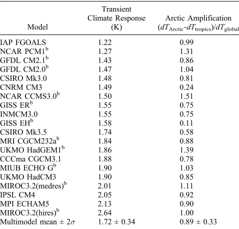
Table 1. Surface Temperature Response of CMIP3 Models for 1pctto2x Simulationsa

Model

Transient Climate Response

(K)

Arctic Amplification (dTArctic‐dTtropics)/dTglobal

IAP FGOALS 1.22 0.99

NCAR PCM1b 1.27 1.31

GFDL CM2.1b 1.43 0.86

GFDL CM2.0b _{1.47 1.04}

CSIRO Mk3.0 1.48 0.81

CNRM CM3 1.49 0.24

NCAR CCMS3.0b 1.50 1.51

GISS ERb _{1.55 0.75}

INMCM3.0 1.55 0.75

GISS EHb _{1.58 0.11}

CSIRO Mk3.5 1.74 0.58

MRI CGCM232ab _{1.84 0.88}

UKMO HadGEM1b _{1.86 1.39}

CCCma CGCM3.1 1.88 0.78

MIUB ECHO Gb _{1.90 1.03}

UKMO HadCM3 1.90 0.85

MIROC3.2(medres)b _{2.01 1.11}

IPSL CM4 2.05 0.92

MPI ECHAM5 2.13 0.90

MIROC3.2(hires)b 2.64 1.00

Multimodel mean ± 2s 1.72 ± 0.34 0.89 ± 0.33

a_{The multimodel ensemble means with 2 standard deviations are also} given. Arctic amplification was taken as the Arctic mean minus tropical mean surface temperature response divided by the global mean surface temperature response.

[10] In order to use equation (2) to break down the 20th century surface temperature response into these components, the total feedback, the Planck feedback and the 20th century forcing are required. The total feedback parameter was determined from simulations forced with a 1% annual increase in CO2to the point of doubling (1pctto2x) where we

know the forcing reasonably accurately. Equation (1) was used in the zonal mean to obtain the total zonal mean

feed-back parameter by regressingDR−FagainstDTsover the

time when the forcing is changing. The regression method allows for latitudinally dependent rapid atmospheric

adjust-ments to the forcing [Gregory et al., 2004;Forster and

Taylor, 2006; Gregory and Webb, 2008;Andrews and Forster, 2008] that are traditionally included in the feed-back term. This has been shown to produce a feedfeed-back parameter that is much more independent of the forcing

mechanism than using the instantaneous or stratosphere‐

adjusted forcing [Shine et al., 2003; Hansen et al., 2005;

Crook et al., 2011] and is also more time independent [Williams et al., 2008]. For these reasons, our assumption that 1pctto2x feedback parameters can be applied to the 20th century is reasonable [seeForster and Taylor, 2006]. Using the regression method means our 20th century forcing term will also include rapid atmospheric adjustments. We chose to use zonal means because smaller spatial scales show more nonlinearities but using larger spatial scales would cause problems because of changing spatial coverage in the observations over the 20th century, and different forcing patterns in the 20th century compared to 1pctto2x simulations [seeCrook et al., 2011].Myhre et al.[1998] showed that the forcing due to CO2takes the form

F¼lnC C0

; ð3Þ

where C is the current concentration and C0 is the initial

concentration of CO2and in our caseais a function of

lati-tude. A small number of CMIP3 models provide TOA stratosphere‐adjusted forcing for 2 × CO2(National Center

for Atmospheric Research (NCAR) CCSM3.0, GISS ER, Meteorological Research Institute (MRI) CGCM2.3.2a, and

Institut Pierre‐Simon Laplace (IPSL) CM4). Equation (3)

with C

C0¼2was used to determineafor each of these

mod-els and the ensemble mean a was used to determine the

forcing for the 1pctto2x scenario. The 1pctto2x forcing in yearyis given by

Fy¼yln 1ð :01Þ: ð4Þ

[11] The partial radiative perturbation method with the Edwards Slingo radiation code [seeCrook et al., 2011] was used to find the Planck feedback parameter for a subset of the models (Geophysical Fluid Dynamics Laboratory (GFDL) CM2.1, NCAR CCSM3.0, GISS EH, UK Met Office (UKMO) HadGEM1 and MIROC3.2(medres); these were simply the first of the models we analyzed). Temperature and humidity profiles for the 1pctto2x case were taken as the 30 year mean after the point of doubling of CO2(year 70).

Although calculations were performed for all sky conditions,

the model’s cloud profile was not included as this would

be treated differently in each model’s own radiation code.

The Planck feedback parameter for these models is very similar and, therefore, the exercise was not repeated for the remaining models. For all models the ensemble mean Planck feedback parameter was used in analysis of 20th century simulations.

[12] Equation (1) was then used to determine the 20th century zonal mean forcing in each model using the total zonal mean 1pctto2x feedback parameter and the 20th cen-tury total temperature response and TOA net downward radiative flux change. Finally the partial temperature response time series was determined using equation (2) in the zonal mean. Surface temperature observations have a considerable amount of missing data, especially during the early part of the 20th century. Given that we are comparing modeled 20th century temperature responses with observations, only the locations with valid observations must be included in the determination of zonal means at each point in time. There-fore interpolation and masking was performed on the total temperature response and TOA net downward radiative flux change before taking zonal means. Note that internal vari-ability will form a part of all three components of tempera-ture response. Some of this variability can be eliminated by taking ensemble means of a number of simulations for each model.

2.3. Linear Trend Comparisons

[13] Linear regression was used to obtain trends for the global mean, Arctic (60°N–90°N) mean and tropical (30°S– 30°N) mean surface temperature response over the whole time period available for all models (1900–1999) and over the two particularly strong warming periods (1918–1940 and 1965–1999) seen in the observations. We used linear trends rather than simple differences between two time periods to reduce the effect of strong or weak responses to the volcanic eruptions of 1902, 1963, and 1991. None of the models has more than five simulations for the 20th century, and so most models do not give us a good sense of the likely spread of possible trends because of internal variability. Therefore, control data from all CMIP3 models were used to assess whether each model has an adequate representation of the observed warming in these regions in each of these time periods within expected internal variability. This assumes that the control data contain an adequate measure of internal variability. Models generally reproduce the large‐scale pat-terns of seasonal surface temperature variation, tempera-ture extremes, and the dominant extratropical patterns of variability such as annular modes and the Pacific Decadal Oscillation, but there still remain problems in adequately

representing the El Niño–Southern Oscillation and the

Madden‐Julian Oscillation [Randall et al., 2007]. The control data were divided into sections of the same number of years as each of the three time periods and the same missing data mask as for the observations was applied before determining linear trends.

temperature response centered on the point of doubling of CO2, i.e., year 70, [Cubasch et al., 2001] and the Arctic

amplification was taken as the Arctic mean minus tropical mean surface temperature response divided by the global mean surface temperature response for the same 20 year mean [see Crook et al., 2011]. We use this definition of Arctic amplification rather than a simple ratio of Arctic warming to global mean warming because some components of the temperature response may warm the Arctic more than the tropics and others may warm the tropics more than the Arctic. The TCR and Arctic amplification of the 1pctto2x simula-tions for all CMIP3 models are shown in Table 1. From this it is clear that those models that were analyzed under 20th century forcing (see footnote b in Table 1) cover the range of TCR and Arctic amplification of all CMIP3 models. We do not expect the Arctic amplification to be the same in 1pctto2x and 20th century simulations because the forcing in the 20th century is less homogeneous, but we might expect those models with high Arctic amplification in 1pctto2x to have high Arctic amplification in 20th century simulations.

2.4. Optimal Fingerprint Analysis

[15] Given that the climate models include internal vari-ability and there are only a small number of realizations available of each one, total least squares (TLS) optimal regression was used to allow for noise in the model data [Stott et al., 2003]:

y¼Xðxi viÞiþv0; ð5Þ

where y are the observations (in our case the optimized

observed temperature anomaly),xiare the modeled responses (in our case the optimized components of the total tempera-ture anomaly),niis the noise in the modeled responses,n0is

the noise in the observations, andbiare the scaling factors.

For the optimal fingerprint analysis, 5 year means from 1900 to 1999 were used as all the models chosen cover this time period. The model data and HadCRUT3 data set were con-verted to anomalies from the 1900–1999 mean. Control data from as many CMIP3 models as possible were used to pro-vide the estimates of internal variability required by the optimal fingerprint analysis code. This gave us 2 independent sets of 42 segments of nonoverlapped control data. One set was required for the“prewhitening”operator, which is used to produce the optimized fingerprints from the temperature anomaly components, and the second set was required for the model consistency checks [Allen and Tett, 1999], allowing us to perform the analysis with up to the first 42 eigenvectors of internal variability (truncation of 42). The analysis was per-formed on the ensemble mean of all the available runs for each model for 30° latitude band means using truncations 2 to 42 and global means using truncations 2 to 19 (note that the global mean data has a vector size of 20 and therefore only 19 eigenvectors are needed). We do not make any assumptions on the best number of truncations to use, although it is probably best to use more than 4, but we present results for a range of truncations. The consistency checks can indicate when the number of truncations is unsuitable. It was not possible to detect all three components of temperature response in one regression. We therefore combined two at a time and performed the regression analysis ondTforcingand

dTfeedback+dTheat,dTfeedbackanddTforcing+dTheat, anddTheat

and dTforcing + dTfeedback so that our regression equations become

dTobs¼ dTf orcing vf orcing

f orcing

þðdTf eedbackþdTheat vremainderÞremainderþv0; ð6Þ

dTobs¼ðdTf eedback vf eedbackÞf eedback

þ dTf orcingþdTheat vremainder

remainderþv0; ð7Þ

dTobs¼ðdTheat vheatÞheat

þ dTf eedbackþdTf orcing vremainder

remainderþv0: ð8Þ

[16] Our aim in this analysis was to see if we could dis-tinguish between models through their different contributions to temperature response, but we also performed the analysis for the multimodel mean results.

3.

Results and Discussion

3.1. Global Mean Linear Trend Comparisons

[17] The linear trends in the global mean temperature response of the models over the 20th century are given in Table 2. Using 84 sections of 100 years of control data from all CMIP3 models, the observed trend over the whole time

period was found to be within the model ensemble mean ±2s

for all models except MIROC3.2(medres), which has too little warming. NCAR CCSM3 has a warming trend on the upper limit and GISS ER has a warming trend on the lower limit.

[18] The global mean trends over the 20th century are not in the same order as for 1pctto2x (see Table 2 and Figure 1a). For example, one might expect the high climate sensitivity MIROC3.2(medres) model to show one of the greatest warming trends over the 20th century but in fact it shows the least, and NCAR CCSM3.0, a model of low to middle climate sensitivity, shows the greatest warming trend. This is due to the fact that these models have not included the same forcings over the 20th century, varying in whether they include ozone, black carbon, organic carbon, mineral dust, sea salt, land use changes and the indirect effects of sulphate aerosols.Kiehl

[2007] and Knutti [2008] pointed out how surprising it is

contribu-tions to the temperature response. MIROC3.2(hires) has a stronger than expected forcing contribution compared to its TCR because of its strong heat storage in the 20th century. Not including MIROC3.2(hires), we found a weak anti-correlation betweendTforcingand TCR of−0.30 (Figure 1b). Knutti[2008] found a similar anticorrelation between global mean forcing and climate sensitivity. The global mean linear trends in temperature response due to the feedback, expressed as a fraction of the total (Table 2), are unsurprisingly more in line with the TCR of the model, although the latitudinal pattern of forcing affects this. The temperature response contributions due to the forcing and due to the feedback have similar standard deviations between models (Table 2)

showing the importance of both the differences in the forcing and in the climate sensitivity between models. It should be noted that the forcing contribution includes rapid atmospheric adjustments which can be quite different in different models, and the standard deviation between models in their instanta-neous forcing (if that were available) would likely be much smaller.

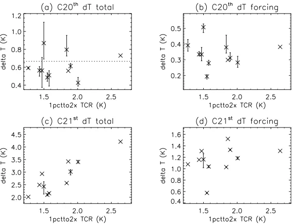
[19] Contributions to the temperature response for up to three simulations (where available) of each model under the SRES A1B emissions scenario were calculated. In contrast to the 20th century warming, the projected warming for the 21st century is positively correlated with the TCR of the model (Figures 1a and 1c). There are considerable differences

Figure 1. Comparison of 20th century and 21st century projected (SRES A1B) global mean warming trends with transient climate response from 1pctto2x experiments: (a) 20th century total global warming trend, (b) 20th century forcing contribution to the global mean warming trend, (c) 21st century total global warming trend, and (d) 21st century forcing contribution to the global mean warming trend. Crosses show the mean trend, and vertical error bars show the range of trends of the simulations for each model. The dotted horizontal line shows the 20th century observed global mean warming trend.

Table 2. Global Mean Surface Temperature Response (Total and Contributions) for 20th Century Simulations Expressed as a Linear Trend Over the Whole Time Perioda

Model

(Simulations Included in Ensemble Mean)

dTtotal (K)

dTforcing (K)

dTfeedback (K)

dTheat (K)

NCAR PCM1 (2) 0.59 0.39 (0.66) 0.35 (0.60) −0.15 (−0.26)

GFDL CM2.1 (3) 0.56 0.33 (0.59) 0.35 (0.57) −0.09 (−0.17)

GFDL CM2.0 (3) 0.56 0.33 (0.59) 0.35 (0.61) −0.12 (−0.22)

NCAR CCSM3.0 (5) 0.87 0.51 (0.58) 0.53 (0.61) −0.17 (−0.20)

GISS ER (5) 0.49 0.19 (0.30) 0.41 (0.85) −0.12 (−0.25)

GISS EH (5) 0.51 0.28 (0.55) 0.32 (0.62) −0.08 (−0.16)

MRI CGCM2.3.2a (5) 0.80 0.38 (0.48) 0.54 (0.68) −0.13 (−0.16)

UKMO HadGEM1 (1) 0.56 0.30 (0.53) 0.36 (0.65) −0.10 (−0.18)

MIUB ECHO‐G (3) 0.61 0.31 (0.51) 0.37 (0.60) −0.07 (−0.11)

MIROC3.2(medres) (3) 0.43 0.28 (0.66) 0.33 (0.76) −0.18 (−0.43)

MIROC3.2(hires) (1) 0.73 0.38 (0.52) 0.56 (0.77) −0.22 (−0.29)

Multimodel mean ±2s 0.61 ± 0.27 0.34 ± 0.16 0.41 ± 0.19 −0.13 ± 0.09

Observations ±2s 0.67 ± 0.08 ‐ ‐ ‐

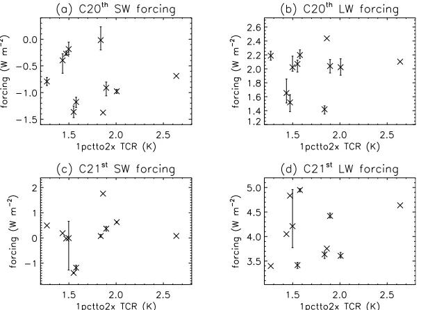
between models in the SRES A1B forcing and there is a weak positive correlation betweendTforcingand TCR of 0.36 (Figure 1d) that enhances the relationship between tempera-ture response and TCR. The forcing differences were further analyzed by examining the linear trends of the shortwave and longwave forcing components (Figure 2). The 20th century shortwave forcing trend is negative in all models, whereas in the 21st century the shortwave forcing trend is positive in some models and negative in others resulting in large dif-ference between models. In the 20th century the short-wave forcing is dominated by volcanic eruptions, although anthropogenic aerosols increase, giving a negative shortwave forcing. However, in the 21st century there are no volcanic eruptions specified and we expect the shortwave forcing to be dominated by decreasing anthropogenic aerosols. The SRES A1B scenario specifies sulphur emissions, but nonsulphate aerosols and whether the indirect effect of aerosols is included is left to the discretion of the modeling centers. Shortwave forcing is affected by the direct effect of aerosols, but both shortwave and longwave forcings are affected by the rapid tropospheric adjustments (semidirect effect) to the aerosol forcing and indirect effects to clouds which will be different in each model. The different aerosol forcings cause conver-gence of modeled temperature response in the 20th century, but divergence in the 21st century.

[20] Attempts to constrain climate sensitivity and future projected warming in multimodel ensembles by weighting models on the basis of their skill in reproducing recent past climate have not been very successful and there is no consensus on how best to obtain model weights [Weigel et al., 2010]. Climate sensitivity has been constrained using model weighting in perturbed physics parameter ensembles and in energy balance models [Hegerl et al., 2007] to some extent, although the upper limit is still poorly constrained. The

cli-mate sensitivity of CMIP3 models typically has a narrower range and lies within these limits. Our results show that for CMIP3 models, skill in reproducing 20th century global mean temperature response is unrelated to both TCR and 21st century global mean temperature response because of the differences in aerosol forcing in models. The measure of skill in reproducing 20th century global mean temperature response (and possibly other climate variables) is more a measure of how well the CMIP3 model has been tuned to fit the observations given its included forcing, rather than how well its climate sensitivity matches that of the real world, which helps to explain why constraining climate sensitivity by weighting multimodel ensembles has not been very suc-cessful. However, measuring skill in producing the green-house gas contribution to the 20th century warming is useful in constraining future warming [Stott et al., 2006].

3.2. Arctic and Tropics Trend Comparisons

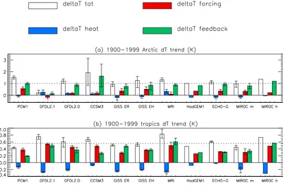
[21] The total response of the models and the contributions over the whole 20th century in terms of the linear trend in the Arctic and tropics are shown in Figure 3. All three temper-ature response contributions for both Arctic and tropics vary considerably between models and have the same order of magnitude in their standard deviation (Table 3). Relative warming between Arctic and tropics is highly dependent on the latitudinal distribution of the forcing, which varies between models, and is much less dependent on the Arctic amplification in 1pctto2x. The Arctic and topics trends over the two rapid warming periods (1918–1940 and 1965–1999) and their contributions in these periods are shown in Figure 4. [22] Using 84 sections of 100 years of control data from all CMIP3 models to assess the role of internal variability, the

observed 1900–1999 trends in both the Arctic and tropics

were found to be within ±2sfor eight of the eleven models.

However, there are three models for which this is not the case and another two models in which the relative warming in the Arctic compared to the tropics is probably unrealistic. We now discuss these five models in detail. Although both

NCAR models have plausible 1900–1999 Arctic and tropics

trends, the tropical warming for NCAR PCM1 is on the low side and the Arctic warming for NCAR CCSM3.0 is on the high side. There were no simulations that gave a warming less than or equal to the observed trend in the Arctic at the same time as a warming greater than or equal to the observed trend in the tropics, implying that both these models tends to pro-duce too much warming in the Arctic compared to the tropics. For NCAR PCM1 both the forcing and feedback contribu-tions to the temperature response are considerably higher in the Arctic than the tropics leading to this high Arctic ampli-fication. This model also had a high Arctic amplification in 1pctto2x and shows strong Arctic amplification in both early and late warming periods (Figure 4). In fact the observed 1965–1999 Arctic trend is outside ±2s, being considerably lower than the modeled trend. For NCAR CCSM3.0 the high Arctic amplification is due to the high feedback in the Arctic compared to the tropics. This model had the highest Arctic amplification in 1pctto2x. For this model the 1pctto2x feed-back parameters were obtained individually for the albedo feedback, shortwave cloud feedback, water vapor plus lapse rate feedback and longwave cloudy sky feedback, and the partial temperature contributions due to each of these

feed-backs were calculated using the method described byCrook

et al.[2011] for both the 1pctto2x run and the 1st run of the 20th century. The percentage contributions to the Arctic amplification from the forcing, heat storage and transport and

the individual feedbacks are given in Table 4. In both forcing scenarios, the albedo feedback, water vapor plus lapse rate feedback, and longwave cloudy sky feedback provide a similar positive contribution to the Arctic amplification; the shortwave cloud contribution is only weakly negative.Crook et al. [2011] also found a weak negative shortwave cloud contribution for the equivalent slab ocean model forced with 2 × CO2, whereas for many other models, there was a strong

negative shortwave cloud contribution.

[23] The observed 1900–1999 trends in the tropics are

outside ±2s for GFDL CM2.1; the model has too much

warming in the tropics. There were no simulations where the warming was greater than or equal to the observed trend in the Arctic at the same time as being less than or equal to the observed trend in the tropics, implying this model pro-duces too little warming in the Arctic compared to the tro-pics. This model has a strong response to volcanic forcing, particularly to Krakatau in 1983 [Knutson et al., 2006], even without including the aerosol indirect effect. In the tropics,

Figure 3. Contributions to the modeled temperature response in (a) the Arctic and (b) the tropics over the 1900–1999 period. Vertical error bars show the range of trends from the simulations for each model. The dotted horizontal lines show the observed warming trends for comparison.

Table 3. Multimodel Ensemble Mean ( ±2 Standard Deviations) Surface Temperature Response (Total and Contributions) in the Arctic and Tropics Expressed as a Linear Trend Over the Whole 20th Century

Arctic Tropics

dTtotal(K) 1.16 ± 0.85 0.60 ± 0.27

dTforcing(K) 0.27 ± 0.41 0.39 ± 0.20

dTfeedback(K) 0.90 ± 0.71 0.39 ± 0.26

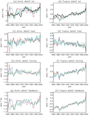
the temperature anomaly recovers only gradually from this cooling effect, with another small cooling presumably due to Santa Maria in 1902, and is still considerably lower than observations in the first decade of the 20th century (Figure 5b). This may account for the large 20th century tropical warming trend. In the Arctic, however, although the influence of Krakatau can be seen, the temperature anomaly recovers very rapidly, resulting in an unusually high anomaly at the beginning of the century, and any cooling due to Santa Maria or Katmai (1912) is not enough to bring the anomaly in line with observations at this time (Figure 5a). This is the only model which has a negative forcing trend in the Arctic over the whole 20th century. The Arctic forcing contribution shows a gradual decrease from 1920 until the 1970s at which point it shows an increase (Figure 5e).Knutson et al.[2006] pointed out that this model has particularly large internal variability. Although the rapid warming from the 1890s to

1920 is likely due to recovery from the Krakatau eruption plus internal variability, the subsequent decrease in Arctic forcing until the 1970s is most likely due to negative aerosol forcing outweighing positive greenhouse gas forcing (note this does not appear to be the case in the tropics).

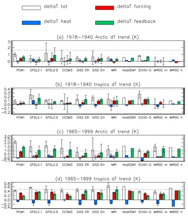
Figure 4. Contributions to the modeled temperature response in (a, c) the Arctic and (b, d) the tropics during the two warming periods, 1918–1940 and 1965–1999. Vertical error bars show the range of trends from the simulations for each model. The dotted horizontal lines show the observed warming trends for comparison.

Table 4. Percentage Arctic Amplification Contributions Due to Forcing, Heat Storage and Transport, and the Different Feedbacks for the 1pctto2x and 20th Century NCAR CCSM3.0 Runs

1pctto2x 20th Century Run 1

Forcing −0.23 −0.05

Heat 0.15 −0.05

Surface albedo 0.38 0.39

Shortwave cloud −0.07 −0.07

Water vapor + lapse rate 0.43 0.43

[24] The observed 1900–1999 trends in the tropics are

outside ±2sfor MRI CGCM232a; the model has too much

warming in the tropics. There were no simulations where the warming was greater than or equal to the observed trend in the Arctic at the same time as being less than or equal to the observed trend in the tropics, implying this model produces too little warming in the Arctic compared to the tropics. The model is cooler in the tropics than observations pre‐1910 and then warms quite strongly in the latter part of the 20th century due to strong forcing and feedback contributions. The forcing contribution in the Arctic is very small and warming here is largely caused by heat transport from the tropics.

[25] The observed 1900–1999 trends in the tropics are

outside ±2s for MIROC3.2(hires); the model has too much

warming in the tropics. There were no simulations where the warming was greater than or equal to the observed trend in the Arctic at the same time as being less than or equal to the observed trend in the tropics, implying this model produces too little warming in the Arctic compared to the tropics. However, it should be noted that we only had one simulation for this model from which to produce a model mean. The 1918–1940 warming trends in both the Arctic and tropics are too low (Figure 4) because of very little forcing; in fact the Arctic cools slightly in the early period. Increasing

warming occurs post‐1940 in both regions because of strong feedback in the Arctic and strong forcing in the tropics.

3.3. Early Warming Trend Comparisons

[26] Figure 4 shows that the 1918–1940 warming in both

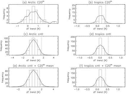
the Arctic and tropics is not well captured by most models. However, the history of warming prior to 1940 followed by cooling, followed by further warming from the 1960s, seen in the observations, and which is much more distinct in the Arctic than the tropics, is found in models to some extent. To ascertain the role of internal variability in the early warming, 366 control sections of 22 years were used with the same

missing data mask applied as for the 1918–1940

observa-tions. Probability distribution functions were produced for the Arctic and tropics mean warming trends of all 20th century simulations (Figures 6a and 6b), of all control simulations (Figures 6c and 6d), and of all control simulations plus the multimodel mean warming trend from 20th century simula-tions (Figures 6e and 6f). This shows that it is exceedingly unlikely that the early warming was due to internal variability alone (both Arctic and tropics observed trends are outside ±2sfor controls) and that the observed trends are still at the upper end of the 20th century modeled trends which include some forced contribution. When comparing the 366 control trends plus the multimodel mean 20th century trend, it is found that the Arctic is just within ±2sand the tropics is not. Repeating this for each model mean, it is found that only

GFDL CM2.1, UKMO HadGEM1 and MIUB ECHO‐G have

adequate warming in the tropics. Therefore, assuming control runs reproduce multidecadal internal variability realistically, it is unlikely that internal variability can explain the differ-ence between the multimodel mean 20th century trend and the observed trend in the tropics, and likely that many models are missing some positive forcing or have too much negative forcing here during this time. In the Arctic there is more internal variability than in the tropics and so we cannot rule out that internal variability (albeit a large realization of it) can explain the difference between observations and each model except in the case of MIROC3.2(medres) and MIROC3.2 (hires). Certainly in the MIROC3.2 models more positive forcing would be needed to simulate the observed trends.

[27] Wang et al. [2007] suggested Arctic early warming was consistent with internal variability in some but not all CMIP3 models, but they looked at mean anomalies over 1939–1949 rather than looking at trends. They also noted that whereas the observed warming was multidecadal, the mod-eled warming was only decadal. Although our results broadly agree with this, we wish to stress that a large warming response due to internal variability is required to match trends

in the Arctic. Delworth and Knutson [2000] used trends

from their older GFDL model and also concluded that only an unusually large realization of internal variability on top of greenhouse gas and sulphate aerosol forcing could have produced the early 20th century warming, although they

could not quantify contributions from natural forcing. The

more recent study of Knutson et al.[2006] on the CMIP3

versions of the GFDL models suggests that the observed early global mean warming can be produced by a combination of anthropogenic forcing and natural forcing, or either anthro-pogenic forcing or natural forcing only in combination with an unusually strong warming from internal variability, but it should be noted that GFDL CM2.1 was one of only three

models with adequate tropical early warming.Shindell and

Faluvegi [2009] showed that internal variability and a net positive aerosol forcing on top of the greenhouse gas, ozone

and natural forcing was required to match 1890–1930

increases in the Arctic minus SH extratropics gradient. They also inferred a net negative aerosol forcing in the tropics over this time. Our results suggest it is likely that many CMIP3 models have too much negative aerosol forcing in the tropics from 1918 to 1940, and, although eight of the models do include black carbon, it is possible that they do not include enough, or they have too strong an aerosol indirect effect. Another possibility may be that some models do not cool enough in response to the 1883, 1902 and 1912 volcanic eruptions and, therefore, have less to recover from subse-quently. Because of a lack of observations, the global distri-bution of aerosol optical depth has to be estimated for these eruptions and this is highly dependent on the circulation patterns at the time of the eruption as well as the amount of SO2ejected. Many models use theSato et al.[1993] volcanic

data set where simple assumptions have been made about distributions. TheAmmann et al.[2003] data set used by the NCAR models attempts to improve the estimates of aerosol optical depth for the early volcanoes by estimating the spread and decay of the aerosol according to the seasonal strato-spheric transport.

[28] Errors in the observed temperature anomalies were not taken into account in our comparisons. Correcting for biases in the instrumental record due to differences in the way sea surface temperatures were measured during the Second World War is expected to only affect temperatures between

1940 and 1960 so our 1918–1940 trends should not be

affected. However, to test this, our calculations could be performed just for land grid boxes or with the corrected CRU temperature data set when it becomes available.

3.4. Optimal Fingerprint Analysis

[29] Detection of components of temperature response proved difficult because of poor signal‐to‐noise ratio and degeneracy between components. This was particularly the case for those models with small response to volcanic forcing compared to noise (MRI CGCM2.3.2a, UKMO HadGEM1, MIROC3.2(medres), and MIROC3.2(hires)) resulting in large uncertainties. Detection was poorer (larger uncertainties) for 30° latitude band means than for global means because the signal to noise is poorer. It was not possible to detect the temperature response due to the feedback (dTfeedback) and

remaining dT (dTforcing + dTheat) for any models or the

multimodel mean in either global mean or 30° latitude band means as uncertainties were too large. This is not surprising in the global mean asdTfeedbackis a scaled version ofdTtotal

and therefore degenerate with it. In general dTfeedback and

the remaining dT are also quite similar compared to the

noise (particularly in the global mean). Sudden changes in

dTforcingfrom volcanic eruptions are opposed bydTheat, so combining these smoothes the combined response. It was possible to detectdTforcingand the remainingdT(dTfeedback+

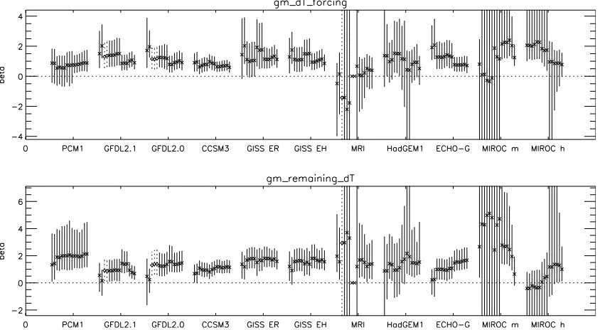
dTheat) for many models in both global means and 30° latitude band means (Figure 7 shows the global mean results) and

to detectdTheatand remainingdT(dTforcing+dTfeedback) for some models in the global mean (not shown). For these cases most models pass the consistency checks for the majority of truncations, but more confidence should be put in the results of those models which have similar scaling factors across a wide range of truncations. Unfortunately, we found it was not possible to distinguish scaling factors between models because of large uncertainties. This shows that it is possible to reproduce the 20th century temperature response pattern in different ways through a balance of forcing and feedback. Nevertheless, our results show that the direct radiative tem-perature response due to forcings is detectable in the climate record irrespective of the climate feedbacks.

[30] For the multimodel mean we also performed the

optimal fingerprint analysis on tropical means and 40°N–

60°N means for dTforcinganddTfeedback+dTheatto see how well different regions performed. We used 40°N–60°N rather than the Arctic because detection was very poor in the Arctic where there is less data and more variability. In both regions and the global mean the scaling factors for thedTforcing

con-tribution were close to one, although in the 40°N–60°N

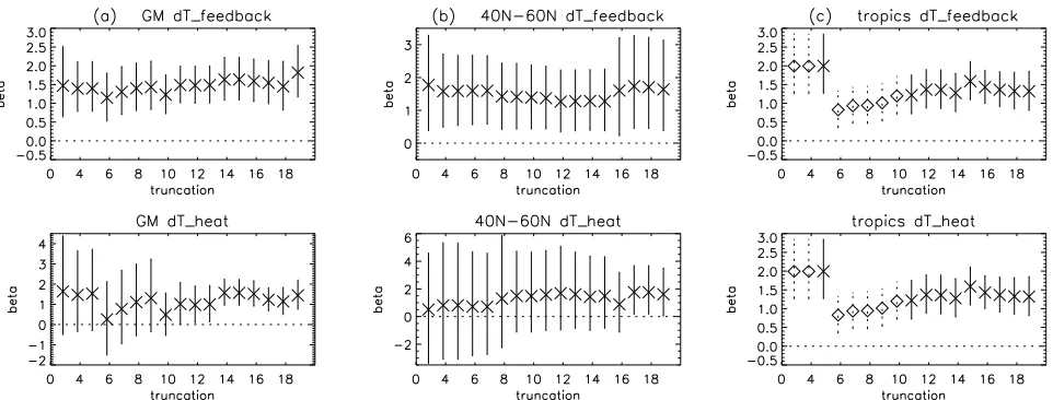
region the uncertainties were larger such that the scaling factors were not inconsistent with zero (the mean scaling factor and their 95% uncertainty ranges over truncations 5–19 for which the consistency test passed were 0.97 ± 0.54 for the global mean, 0.76 ± 0.29 for the tropics and 0.54 ± 2.03 for 40°N–60°N). We then took the scaleddTforcingaway from the observed temperature anomalies so that we could perform an optimal fingerprint analysis of the observed temperature anomaly minus the forcing contribution against the modeled feedback and heat storage and transport contributions. This was our only way to investigate the accuracy of the multi-model mean feedback. The results for these analyses for

global means, tropical means, and 40°N–60°N means are

shown in Figure 8. Scaling factors for thedTheatcontribution are close to one in all these regions. The feedback contribu-tion tends to be underestimated by the multimodel mean,

particularly in the global mean and 40°N–60°N mean where

the scaling factor is close to 1.5 suggesting the real world

feedback may be greater than the multimodel mean feedback, although the uncertainties are such that the scaling factor is consistent with one.

4.

Conclusions

[31] The response of the models over the 20th century in terms of the linear trend in global mean temperature response does not follow the same order as for 1pctto2x because of different 20th century forcing in each model compensating for the climate sensitivity to some extent. Despite being able to detectdTforcingand the remainingdTin most models using optimal fingerprint analysis, we were unable to dis-tinguish between models because of the large uncertainties in the scaling factors. Both these results highlight the difficulty of constraining climate sensitivity when there is so much uncertainty in 20th century forcing. If 20th century forcing could be better constrained and models run under such a forcing scenario this may lead to a better understanding of which models produce the most accurate response and therefore could constrain the feedback and hence climate sensitivity. Modeling groups have been adding missing for-cings to their models for the CMIP5 experiments, potentially allowing for easier comparison between models. Results from these experiments may shed interesting light on the current understanding of 20th century forcing and feedback.

[32] In contrast to the 20th century, projected global mean warming over the 21st century is much more dependent on the TCR. Whereas differences in aerosol forcing cause con-vergence of temperature response in the 20th century, dif-ferences in the 21st century cause divergence, making it very difficult to constrain climate sensitivity and future predictions of climate change by weighting the CMIP3 models according to their 20th century skill. Better understanding of aerosol forcing is therefore of great importance.

[33] A comparison of modeled and observed warming trends in the Arctic and tropics suggests the tropical warming is too high and Arctic amplification is too low in GFDL CM2.1, MRI CGCM232a, and MIROC3.2(hires) because of

Figure 8. Best estimate of scaling factors (crosses or diamonds) and their 5%–95% uncertainty estimates

(vertical lines) for optimal regression of the multimodel mean (top)dTfeedbackand (bottom)dTheatin

too little forcing in the Arctic compared to the tropics. The Arctic amplification in NCAR PCM1 and NCAR CCSM3.0 is unrealistically high because of high feedback contributions in the Arctic compared to the tropics in both these models and also because of a high forcing contribution in NCAR PCM1. It is also evident that few of the models produce the early (1918–1940) warming, particularly in the tropics and that internal variability is unlikely to explain the difference, sug-gesting many models are missing some positive forcing or have too much negative forcing at this time. Variability is higher in the Arctic and so it is not possible to state the need for more positive forcing here, although a larger positive forcing in the tropics would also cause more warming in the Arctic through increased heat transport from the tropics. The larger positive forcing may be due to more black carbon, a smaller aerosol indirect effect than is currently included in models, or stronger volcanic forcing at the beginning of the 20th century.

[34] Finally, our multimodel mean optimal fingerprint analysis results suggest that the multimodel mean forcing contribution to the temperature response is quite well detected

in global means, 40°N–60°N means and tropical means, but

the feedback is lower in these regions than observed tem-perature anomalies suggest.

[35] Acknowledgments. We acknowledge the modeling groups, the Program for Climate Model Diagnosis and Intercomparison (PCMDI), and the WCRP’s Working Group on Coupled Modeling (WGCM) for their roles in making available the WCRP CMIP3 multimodel data set. Support of this data set is provided by the Office of Science, U.S. Department of Energy. We also acknowledge CRU, University of East Anglia, for the HadCRUT3 data set. We thank Nathan Gillett and Daithi Stone for their invaluable advice on the use of the attribution and detection code and inter-pretation of its output. We thank the authors of the attribution code, Myles Allen and Daithi Stone, for allowing us to use the code. Finally, we thank Retto Knutti, Drew Shindell, and one anonymous reviewer for their helpful review comments. This work was funded by NERC grant NE/E016189/1,

“An Observationally‐Based Quantification of Climate Feedbacks.”

References

Allen, M. R., and P. A. Stott (2003), Estimating signal amplitudes in opti-mal fingerprinting, part I: Theory,Clim. Dyn.,21, 477–491, doi:10.1007/ s00382-003-0313-9.

Allen, M. R., and S. F. B. Tett (1999), Checking for model consistency in optimal fingerprinting,Clim. Dyn.,15, 419–434, doi:10.1007/ s003820050291.

Ammann, C. M., G. A. Meehl, W. M. Washington, and C. S. Zender (2003), A monthly and latitudinally varying volcanic forcing dataset in simulations of 20th century climate,Geophys. Res. Lett.,30(12), 1657, doi:10.1029/2003GL016875.

Andrews, T., and P. M. Forster (2008), CO2forcing induces semi‐direct effects with consequences for climate feedback interpretations,Geophys. Res. Lett.,35, L04802, doi:10.1029/2007GL032273.

Boer, G. J., and B. Yu (2003), Climate sensitivity and response,Clim. Dyn.,

20, 415–429.

Bony, S., et al. (2006), How well do we understand and evaluate climate change feedback processes?,J. Clim.,19, 3445–3482, doi:10.1175/ JCLI3819.1.

Brohan, P., J. J. Kennedy, I. Harris, S. F. B. Tett, and P. D. Jones (2006), Uncertainty estimates in regional and global observed temperature changes: A new dataset from 1850,J. Geophys. Res.,111, D12106, doi:10.1029/2005JD006548.

Crook, J. A., P. M. Forster, and N. Stuber (2011), Spatial patterns of modelled climate feedback and contributions to temperature response and polar amplification,J. Clim.,24, 3575–3592, doi:10.1175/ 2011JCLI3863.1.

Cubasch, U., et al. (2001), Projections of future climate changes, inClimate Change 2001: The Scientific Basis. Contribution of Working Group I to the Third Assessment Report of the Intergovernmental Panel on Climate

Change, edited by J. T. Houghton et al., pp. 525–582, Cambridge Univ. Press, Cambridge, U. K.

Delworth, T. L., and T. R. Knutson (2000), Simulation of early 20th century global warming,Science,287, 2246–2250, doi:10.1126/ science.287.5461.2246.

Forster, P. M., and K. E. Taylor (2006), Climate forcings and climate sen-sitivities diagnosed from coupled climate model integrations,J. Clim.,

19, 6181–6194, doi:10.1175/JCLI3974.1.

Gregory, J., et al. (2004), A new method for diagnosing radiative forcing and climate sensitivity,Geophys. Res. Lett.,31, L03205, doi:10.1029/ 2003GL018747.

Gregory, J., and M. Webb (2008), Tropospheric adjustment induces a cloud component in CO2 forcing, J. Clim., 21, 58–71, doi:10.1175/ 2007JCLI1834.1.

Hansen, J., et al. (2005), Efficacy of climate forcings,J. Geophys. Res.,

110, D18104, doi:10.1029/2005JD005776.

Hansen, J., R. Ruedy, M. Sato, and K. Lo (2010), Global surface temper-ature change,Rev. Geophys.,48, RG4004, doi:10.1029/2010RG000345. Hasselmann, K. (1979), On the signal‐to‐noise problem in atmospheric response studies, inMeteorology of Tropical Oceans, edited by D. B. Shaw, pp. 251–259, R. Meteorol. Soc., London.

Hasselmann, K. (1997), Multi‐pattern fingerprint method for detection and attribution of climate change,Clim. Dyn.,13, 601–611, doi:10.1007/ s003820050185.

Hegerl, G. C., T. J. Crowley, S. K. Baum, K.‐Y. Kim, and W. T. Hyde (2003), Detection of volcanic, solar and greenhouse gas signals in paleor-econstructions of Northern Hemispheric temperature,Geophys. Res. Lett.,30(5), 1242, doi:10.1029/2002GL016635.

Hegerl, G. C., et al. (2007), Understanding and attributing climate change, inClimate Change 2007: The Physical Science Basis. Contribution of Working Group I to the Fourth Assessment Report of the

Intergovern-mental Panel on Climate Change, edited by S. Solomon et al.,

pp. 663–745, Cambridge Univ. Press, Cambridge, U. K.

Holland, M. M., and C. M. Bitz (2003), Polar amplification of climate change in coupled models,Clim. Dyn.,21, 221–232, doi:10.1007/ s00382-003-0332-6.

Kiehl, J. T. (2007), Twentieth century climate model response and climate s e n s i t i v i t y , G e o p h y s . R e s . L e t t ., 3 4, L 2 2 7 1 0 , d o i : 1 0 . 1 0 2 9 / 2007GL031383.

Knutson, T.R., et al. (2006), Assessment of twentieth‐century regional sur-face temperature trends using the GFDL CM2 coupled models,J. Clim.,

19, 1624–1651, doi:10.1175/JCLI3709.1.

Knutti, R. (2008), Why are climate models reproducing the observed global surface warming so well?,Geophys. Res. Lett.,35, L18704, doi:10.1029/ 2008GL034932.

Meehl, G. A., W. M. Washington, C. M. Ammann, J. M. Arblaster, T. M. L. Wigley, and C. Tebaldi (2004), Combinations of natural and anthropogenic forcings in twentieth‐century climate,J. Clim.,17, 3721–3727, doi:10.1175/1520-0442(2004)017<3721:CONAAF>2.0. CO;2.

Meehl, G. A., et al. (2007), Global climate projections, inClimate Change 2007: The Physical Science Basis. Contribution of Working Group I to the Fourth Assessment Report of the Intergovernmental Panel on Climate Change, edited by S. Solomon et al., pp. 747–845, Cambridge Univ. Press, Cambridge, U. K.

Min, S.‐K., and A. Hense (2006), A Bayesian assessment of climate change using multimodel ensembles. Part I: Global mean surface temperature,

J. Clim.,19, 3237–3256, doi:10.1175/JCLI3784.1.

Myhre, G., E. J. Highwood, K. P. Shine, and F. Stordal (1998), New esti-mates of radiative forcing due to well mixed greenhouse gases,Geophys. Res. Lett.,25, 2715–2718, doi:10.1029/98GL01908.

Nozawa, T., T. Nagashima, H. Shiogama, and S. A. Crooks (2005), Detecting natural influence on surface air temperature change in the early twentieth century, Geophys. Res. Lett.,32, L20719, doi:10.1029/ 2005GL023540.

Randall, D. A., et al. (2007), Climate models and their evaluation, in Cli-mate Change 2007: The Physical Science Basis. Contribution of Working Group I to the Fourth Assessment Report of the Intergovernmental Panel

on Climate Change, edited by S. Solomon et al., pp. 589–662,

Cambridge Univ. Press, Cambridge, U. K.

Sato, M., J. E. Hansen, M. P. McCormick, and J. B. Pollack (1993), Strato-spheric aerosol optical depths, 1850–1990,J. Geophys. Res.,98(D12), 22,987–22,994, doi:10.1029/93JD02553.

Shindell, D., and G. Faluvegi (2009), Climate response to regional radia-tive forcing during the twentieth century,Nat. Geosci.,2, 294–300, doi:10.1038/ngeo473.

of climate change mechanisms,Geophys. Res. Lett.,30(20), 2047, doi:10.1029/2003GL018141.

Stone, D. A., M. R. Allen, P. A. Stott, P. Pall, S.‐K. Min, T. Nozawa, and S. Yukimoto (2009), The detection and attribution of human influence on climate,Annu. Rev. Environ. Resour.,34, 1–16, doi:10.1146/annurev. environ.040308.101032.

Stott, P. A., S. F. B. Tett, G. S. Jones, M. R. Allen, J. F. B. Mitchell, and G. J. Jenkins (2000), External control of 20th century temperature by nat-ural and anthropogenic forcings,Science,290, 2133–2137, doi:10.1126/ science.290.5499.2133.

Stott, P. A., M. R. Allen, and G. S. Jones (2003), Estimating signal ampli-tudes in optimal fingerprinting. Part II: Application to general circulation models,Clim. Dyn.,21, 493–500, doi:10.1007/s00382-003-0314-8. Stott, P. A., J. F. B. Mitchell, M. R. Allen, T. L. Delworth, J. M. Gregory,

G. A. Meehl, and B. D. Santer (2006), Observational constraints on past attributable warming and predictions of future global warming,J. Clim.,

19, 3055–3069, doi:10.1175/JCLI3802.1.

Thompson, D. W. J., J. J. Kennedy, J. M. Wallace, and P. D. Jones (2008), A large discontinuity in the mid‐twentieth century in observed global‐

mean surface temperature, Nature, 453, 646–649, doi:10.1038/ nature06982.

Trenberth, K. E., et al. (2007), Observations: Surface and atmospheric climate change, inClimate Change 2007: The Physical Science Basis. Contribution of Working Group I to the Fourth Assessment Report of the Intergovernmental Panel on Climate Change, edited by S. Solomon et al., pp. 237–336, Cambridge Univ. Press, Cambridge, U. K. Wang, M., J. E. Overland, V. Kattsov, J. E. Walsh, X. Zhang, and

T. Pavlova (2007), Intrinsic versus forced variation in coupled climate model simulations over the Arctic during the twentieth century,J. Clim.,

20, 1093–1107, doi:10.1175/JCLI4043.1.

Weigel, A. P., R. Knutti, M. A. Liniger, and C. Appenzeller (2010), Risks of model weighting in multimodel climate projections,J. Clim.,23, 4175–4191, doi:10.1175/2010JCLI3594.1.

Williams, K. D., W. J. Ingram, and J. M. Gregory (2008), Time variation of effective climate sensitivity in GCMs,J. Clim.,21, 5076–5090, doi:10.1175/2008JCLI2371.1.