Constraints on the unitarity triangle angle γ from Dalitz plot analysis of B⁰→DK+π− decays

Constraints on the unitarity triangle angle

γ

from Dalitz plot

analysis of

B

→

DK

π

decays

R. Aaijet al.* (LHCb Collaboration)

(Received 11 February 2016; published 30 June 2016)

The first study is presented of CP violation with an amplitude analysis of the Dalitz plot of B0→DKþπ− decays, with D→Kþπ−, KþK−, and πþπ−. The analysis is based on a data sample corresponding to3.0fb−1ofppcollisions collected with the LHCb detector. No significantCPviolation effect is seen, and constraints are placed on the angleγ of the unitarity triangle formed from elements of the Cabibbo-Kobayashi-Maskawa quark mixing matrix. Hadronic parameters associated with the B0→DKð892Þ0decay are determined for the first time. These measurements can be used to improve the sensitivity toγof existing and future studies of theB0→DKð892Þ0decay.

DOI:10.1103/PhysRevD.93.112018

I. INTRODUCTION

One of the most important challenges of physics today is understanding the origin of the matter-antimatter asymme-try of the Universe. Within the Standard Model (SM) of particle physics, the CP symmetry between particles and antiparticles is broken only by the complex phase in the Cabibbo-Kobayashi-Maskawa (CKM) quark mixing matrix[1,2]. An important parameter in the CKM descrip-tion of the SM flavor structure is γ≡arg½−VudVub=

ðVcdVcbÞ, one of the three angles of the unitarity triangle formed from CKM matrix elements [3–5]. Since the SM cannot account for the baryon asymmetry of the Universe

[6] new sources of CP violation, that would show up as deviations from the SM, are expected. The precise deter-mination ofγ is necessary in order to be able to search for such small deviations.

The value ofγcan be determined from theCP-violating interference between the two amplitudes in, for example,

Bþ →DKþ and charge-conjugate decays[7–10]. HereD

denotes a neutral charm meson reconstructed in a final state accessible to both D¯0 and D0 decays, that is therefore a superposition of the D¯0 and D0 states produced through

b→cW andb→uW transitions (hereafter referred to as

Vcb and Vub amplitudes). This approach has negligible theoretical uncertainty in the SM [11] but limited data samples are available experimentally.

A similar method based on B0→DKþπ− decays has been proposed[12,13] to help improve the precision. By studying the Dalitz plot (DP)[14]distributions ofB¯0and

B0 decays, interference between different contributions,

such as B0→D2ð2460Þ−Kþ and B0→DKð892Þ0 (Feynman diagrams shown in Fig. 1), can be exploited to obtain additional sensitivity compared to the “ quasi-two-body” analysis in which only the region of the DP dominated by the Kð892Þ0 resonance is selected

[15–17]. The method is illustrated in Fig. 2, where the relative amplitudes of the different channels are sketched in the complex plane. The B0→D¯0K0 (Vcb) amplitude is determined, relative to that forB0→D₂−Kþ decays, from analysis of the Dalitz plot with the neutral D meson reconstructed in a favored decay mode such as

¯

D0→Kþπ−. The Vub amplitude can then be obtained from the difference in this relative amplitude compared to the Vcb only case when the neutral D meson is recon-structed as aCP eigenstate. A nonzero value of γ causes different relative amplitudes for B0 and B¯0 decays, and henceCPviolation. The method allows the determination ofγ and the hadronic parametersrB andδB, which are the relative magnitude and strong (i.e.CP-conserving) phase of theVubandVcbamplitudes for theB0→DK0decay, with only CP-even D decays required to be reconstructed in addition to the favored decays. This feature, which is in contrast to the method of Refs.[7,8]that requires samples of bothCP-even andCP-odd D decays, is important for analysis of data collected at a hadron collider where reconstruction ofD meson decays toCP-odd final states such as K0Sπ0 is challenging. The Dalitz analysis method also has only a single ambiguity (γ↔γþπ, δ_B ↔ δBþπ), whereas the method of Refs. [7,8] has an eight-fold ambiguity in the determination ofγ.

This paper describes the first study ofCPviolation with a DP analysis of B0→DKþπ− decays, with a sample corresponding to 3.0fb−1 of pp collision data collected with the LHCb detector at center-of-mass energies of 7 and 8 TeV. The inclusion of charge conjugate processes is implied throughout the paper except where discussing asymmetries.

*_{Full author list given at the end of the article.}

II. DETECTOR AND SIMULATION

The LHCb detector [18,19] is a single-arm forward spectrometer covering the pseudorapidity range 2<η<5, designed for the study of particles containingborcquarks. The detector includes a high-precision tracking system consisting of a silicon-strip vertex detector surrounding theppinteraction region, a large-area silicon-strip detector located upstream of a dipole magnet with a bending power of about 4 Tm, and three stations of silicon-strip detectors and straw drift tubes placed downstream of the magnet. The tracking system provides a measurement of momentum,p, of charged particles with a relative uncertainty that varies from 0.5% at low momentum to 1.0% at200 GeV=c. The minimum distance of a track to a primary vertex, the impact parameter, is measured with a resolution ofð15þ29=pTÞμm, wherepTis the component of the momentum transverse to

the beam, in GeV=c. Different types of charged hadrons are distinguished using information from two ring-imaging Cherenkov detectors. Photons, electrons, and hadrons are identified by a calorimeter system consisting of scintillating-pad and preshower detectors, an electromagnetic calorimeter and a hadronic calorimeter. Muons are identified by a system composed of alternating layers of iron and multiwire propor-tional chambers. The online event selection is performed by a trigger, which consists of a hardware stage, based on information from the calorimeter and muon systems, fol-lowed by a software stage, in which all charged particles with

pT>500ð300ÞMeV=care reconstructed for 2011 (2012)

data. A detailed description of the trigger conditions is available in Ref.[20].

Simulated data samples are used to study the response of the detector and to investigate certain categories of back-ground. In the simulation,ppcollisions are generated using

PYTHIA [21] with a specific LHCb configuration [22].

Decays of hadronic particles are described by EVTGEN [23], in which final-state radiation is generated using

PHOTOS [24]. The interaction of the generated particles

with the detector, and its response, are implemented using theGEANT4 toolkit[25]as described in Ref.[26].

III. SELECTION

CandidateB0→DKþπ−decays are selected with theD

meson decaying into theKþπ−,KþK−, orπþπ−final state. The selection requirements are similar to those used for the DP analyses of B0→D¯0Kþπ− [27] and B0s→D¯0K−πþ

[28,29]decays, where in both cases only theD¯0→Kþπ−

mode was used.

The more copiousB0→Dπþπ− modes, with neutralD

meson decays to one of the three final states under study, are used as control channels to optimize the selection requirements. Loose initial requirements on the final state tracks and the D and B candidates are used to obtain a visible peak ofB0→Dπþπ−decays. The neutralDmeson candidate must satisfy criteria on its invariant mass, vertex quality, and flight distance from any PV and from the B

candidate vertex. Requirements on the outputs of boosted decision tree algorithms that identify neutral D meson decays, in each of the decay chains of interest, originating from b hadron decays [30,31] are also applied. These requirements are sufficient to reduce to negligible levels potential background from charmlessBmeson decays that

0

B b d

-(2460)

2

D* c

d

+

K s

u

+

W

(a)

0

B b

d

0

(892) K* s

d

0

D c

u

+

W

(b)

0

B b

d

0

(892) K* s

d

0

D u

c

+

W

(c)

FIG. 1. Feynman diagrams for the contributions to B0→DKþπ− from (a) B0→D2ð2460Þ−Kþ, (b) B0→D¯0Kð892Þ0, and (c)B0→D0Kð892Þ0 decays.

Re Im

1

− +1 +2

1

−

+1

+2 0_K*0)

D

→

0

B

(

A

) +

K

2 − *

D

→

0

B

(

A

Re Im

1

− +1 +2

1

−

+1 +2

γ γ

B

δ

) *0

K CP D

→

0

B

(

A

2

) *0

K CP D

→

0

B

(

A

2

) +

K CP 2

− *

D

→

0

B

(

A

2

FIG. 2. Illustration of the method to determineγfrom Dalitz plot analysis ofB0→DKþπ−decays[12,13]: (left) theVcbamplitude for

B0→D¯0K0compared to that forB0→D2−Kþdecay; (right) the effect of theVubamplitude that contributes toB0→DCPK0 and

¯

B0→DCPK¯0decays provides sensitivity toγ. The notationDCPrepresents a neutralDmeson reconstructed in aCPeigenstate, while

D₂−CPdenotes the decay chainD2−→DCPπ−, where the charge of the pion tags the flavor of the neutralDmeson, independently of the mode in which it is reconstructed, so there is no contribution from theVubamplitude.

have identical final states but without an intermediate D

meson. Vetoes are applied to remove backgrounds from B0→Dð2010Þ−Kþ, B0→D∓π, B0s →D−sπþ, and B0_ðsÞ→D0D¯0 decays, and candidates consistent with originating from B0_ðsÞ→D¯0Kπ∓ decays, where the D¯0

has been reconstructed from the wrong pair of tracks. Separate neural network (NN) classifiers[32]for eachD

decay mode are used to distinguish signal decays from combinatorial background. ThesPlottechnique[33], with the B0→Dπþπ− candidate mass as the discriminating variable, is used to obtain signal and background weights,

which are then used to train the networks. The networks are based on input variables that describe the topology of each decay channel, and that depend only weakly on the B

candidate mass and on the position of the candidate in theB

decay Dalitz plot. Loose requirements are made on the NN outputs in order to retain large samples for the DP analysis.

IV. DETERMINATION OF SIGNAL AND BACKGROUND YIELDS

The yields of signal and of several different backgrounds are determined from an extended maximum likelihood fit,

] 2 c ) [MeV/ − π + K D ( m

5200 5400 5600 5800

)

2

c

Weighted candidates / (16 MeV/

0 200 400 600 800 1000 1200 − π + K → D LHCb (a) ] 2 c ) [MeV/ − π + K D ( m

5200 5400 5600 5800

)

2

c

Weighted candidates / (16 MeV/

2 10

3

10 _DLHCb (b)_→K+_π−

] 2 c ) [MeV/ − π + K D ( m

5200 5400 5600 5800

)

2_c

Weighted candidates / (16 MeV/

0 20 40 60 80 100 120 140 160 180 200 220 240 − K + K → D LHCb (c) ] 2 c ) [MeV/ − π + K D ( m

5200 5400 5600 5800

)

2_c

Weighted candidates / (16 MeV/

1 10 2

10 D→K+K−

LHCb (d) ] 2 c ) [MeV/ − π + K D ( m

5200 5400 5600 5800

)

2

c

Weighted candidates / (16 MeV/

0 10 20 30 40 50 60 70 80 90 − π + π → D LHCb (e) ] 2 c ) [MeV/ − π + K D ( m

5200 5400 5600 5800

)

2

c

Weighted candidates / (16 MeV/

1 10 2 10 − π + π → D LHCb (f)

Data Total fit

± π ± K D → (s) 0

B Combinatorial background

Part. comb. background _B(s)0 →D*K±π ± − π + π * ( ) D → 0

B ( )*π+p

D → 0 b Λ p + K * ( ) D → 0 b Λ − K + K * ( ) D → (s) 0 B

in each mode, to the distributions of candidates in B

candidate mass and NN output. Unbinned information on the B candidate mass is used, while each sample is divided into five bins of the NN output that contain a similar number of signal, and varying numbers of background, decays[34,35].

In addition to B0→DKþπ− decays, components are included in the fit to account forB0sdecays to the same final state, partially reconstructed B0_ðsÞ→DðÞKπ∓ back-grounds, misidentified B0→DðÞπþπ−, B0_ðsÞ→DðÞKþK−,

¯

Λ0

b→DðÞp¯πþ, and Λ¯0b→DðÞpK¯ þ decays as well as combinatorial background. The modeling of the signal and background distributions inBcandidate mass is similar to that described in Ref.[27]. The sum of two Crystal Ball functions [36] is used for each of the correctly recon-structedBdecays, where the peak position and core width (i.e. the narrower of the two widths) are free parameters of the fit, while the B0s–B0 mass difference is fixed to its known value [37]. The fraction of the signal function contained in the core and the relative width of the two components are constrained within uncertainties to, and all other parameters are fixed to, their expected values obtained from simulated data, separately for each of the three D samples. An exponential function is used to describe combinatorial background, with the shape param-eter allowed to vary. Because of the loose NN output requirement it is necessary, in the D→Kþπ− sample, to account explicitly for partially combinatorial background where the final stateDKþ pair originates from aBdecay but is combined with a random pion; this is modeled with a nonparametric function. Nonparametric functions obtained from simulation based on known DP distributions[38–44]

are used to model the partially reconstructed and mis-identified B decays.

The fraction of signal decays in each NN output bin is allowed to vary freely in the fit; the correctly reconstructed

B0sdecays and misidentified backgrounds are taken to have the same NN output distribution as signal. The fractions of combinatorial and partially reconstructed backgrounds in each NN output bin are each allowed to vary freely. All yields are free parameters of the fit, except those for misidentified backgrounds which are constrained within expectation relative to the signal yield, since the relative branching fractions[37]and misidentification probabilities

[45]are well known.

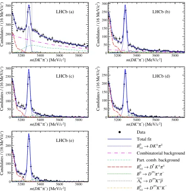
The results of the fits are shown in Fig. 3, in which the NN output bins have been combined by weighting both the data and fit results by S=ðSþBÞ, where S (B) is the signal (background) yield in the signal window, defined as

2.5σðcoreÞ around the B0 peak in each sample, where σðcoreÞ is the core width of the signal shape. The yields of each category in these regions, which correspond to 5246.6–5309.9 MeV=c2, 5246.9–5310.5MeV=c2, and 5243.1–5312.3 MeV=c2 in the D→Kþπ−, KþK−, and

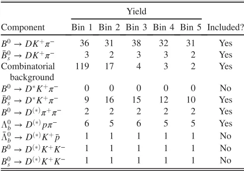
TABLE I. Yields in the signal window of the fit components in the five NN output bins for the D→Kþπ− sample. The last column indicates whether or not each component is explicitly modeled in the Dalitz plot fit.

Component

Yield

Included? Bin 1 Bin 2 Bin 3 Bin 4 Bin 5

B0→DKþπ− 597 546 585 571 540 Yes

B0s →DKþπ− 1 1 1 1 1 No

Combinatorial background

540 58 16 6 1 Yes

Bþ→DðÞKþþX− 305 33 9 3 1 Yes

B0→DKþπ− 1 1 1 1 1 No

B0→DðÞπþπ− 20 18 20 19 18 Yes ¯

Λ0

b→DðÞKþp¯ 21 19 21 20 19 Yes

B0→DðÞKþK− 8 7 8 7 7 No B0s →DðÞKþK− 10 9 10 10 9 No TABLE II. Yields in the signal window of the fit components in the five NN output bins for theD→KþK− sample. The last column indicates whether or not each component is explicitly modeled in the Dalitz plot fit.

Component

Yield

Included? Bin 1 Bin 2 Bin 3 Bin 4 Bin 5

B0→DKþπ− 70 63 68 73 65 Yes ¯

B0s →DKþπ− 5 5 5 6 5 Yes Combinatorial

background

173 19 9 3 0 Yes

B0→DKþπ− 0 1 1 1 0 No

¯

B0s →DKþπ− 19 28 34 28 20 Yes

B0→DðÞπþπ− 4 3 4 4 3 Yes Λ0

b→DðÞpπ− 11 10 10 11 10 Yes

¯

Λ0

b→DðÞKþp¯ 2 1 2 2 2 No

B0→DðÞKþK− 2 1 2 2 1 No B0s →DðÞKþK− 1 1 1 2 1 No

TABLE III. Yields in the signal window of the fit components in the five NN output bins for theD→πþπ− sample. The last column indicates whether or not each component is explicitly modeled in the Dalitz plot fit.

Component

Yield

Included? Bin 1 Bin 2 Bin 3 Bin 4 Bin 5

B0→DKþπ− 36 31 38 32 31 Yes ¯

B0s →DKþπ− 3 2 3 3 2 Yes Combinatorial

background

119 17 4 3 2 Yes

B0→DKþπ− 0 0 0 0 0 No

¯

B0s →DKþπ− 9 16 15 12 10 Yes

B0→DðÞπþπ− 2 2 2 2 2 Yes Λ0

b→DðÞpπ− 6 5 6 5 5 Yes

¯

Λ0

b→DðÞKþp¯ 1 1 1 1 1 No

B0→DðÞKþK− 1 1 1 1 1 No B0s →DðÞKþK− 1 1 1 1 1 No

πþ_π− _{samples, are given in Tables I, II and III. In total,}

there are284070signal decays within the signal window in theD→Kþπ− sample, while the corresponding values for theD→KþK− andD→πþπ− samples are33922 and16819. Theχ2=ndf values for the projections of the fits to the D→Kþπ−, D→KþK−, and D→πþπ− data sets are 171.5=223, 188.2=223, and 169.1=222, respec-tively, giving a totalχ2=ndf ¼528.8=668. Note that there are some bins with low numbers of entries which may result in this value not following exactly the expected χ2 distribution.

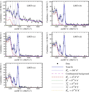
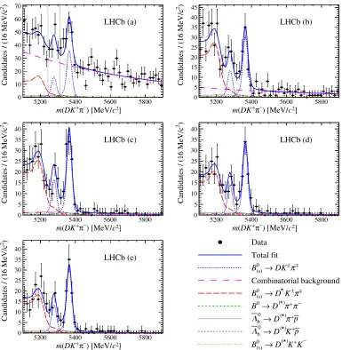
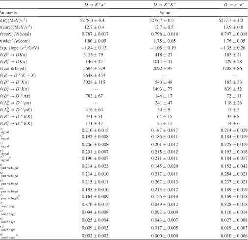
Projections of the fits separated by NN output bin in each sample are shown in Figs. 4–6. The fitted parameters obtained from all three data samples are reported in Table IV. The parameters μðBÞ, NðcoreÞ=NðtotalÞ, σðwideÞ=σðcoreÞ are, respectively, the peak position, the fraction of the signal function contained in the core, and the relative width of the two components of the B0 signal

shape. Quantities denoted N are total yields of each fit component, while those denotedfi

signalare fractions of the

signal in NN output bin i (with similar notation for the fractions of the partially reconstructed and combinatorial backgrounds). The NN output bin labels 1–5 range from the bin with the lowest to highest value ofS=B.

V. DALITZ PLOT ANALYSIS

Candidates within the signal region are used in the DP analysis. A simultaneous fit is performed to the samples with differentDdecays by using theJFIT method[46]as

implemented in the Laura++ package [47]. The likelihood

function contains signal and background terms, with yields in each NN output bin fixed according to the results obtained previously. The NN output bin with the lowest

S=Bvalue in theD→Kþπ− sample only is found not to contribute significantly to the sensitivity and is susceptible

] 2 c ) [MeV/ − π + K D ( m

5200 5400 5600 5800

)

2

Candidates / (16 MeV/c

0 100 200 300 400 500 LHCb (a) ] 2 c ) [MeV/ − π + K D ( m

5200 5400 5600 5800

)

2

Candidates / (16 MeV/c

0 50 100 150 200 250 300 LHCb (b) ] 2 c ) [MeV/ − π + K D ( m

5200 5400 5600 5800

)

2

Candidates / (16 MeV/c

0 50 100 150 200 250 300 LHCb (c) ] 2 c ) [MeV/ − π + K D ( m

5200 5400 5600 5800

)

2

Candidates / (16 MeV/c

0 50 100 150 200

250 _{LHCb (d)}

] 2 c ) [MeV/ − π + K D ( m

5200 5400 5600 5800

)

2

Candidates / (16 MeV/c

0 50 100 150 200 250 LHCb (e) Data Total fit ± π ± K D → (s) 0 B Combinatorial background

Part. comb. background ± π ± K * D → (s) 0 B − π + π * ( ) D → 0 B p + K * ( ) D → 0 b Λ − K + K * ( ) D → (s) 0 B

to mismodeling of the combinatorial background; it is therefore excluded from the subsequent analysis.

The signal probability function is derived from the isobar model obtained in Ref.[27], with amplitude

Aðm2ðDπ−Þ; m2ðKþπ−ÞÞ

¼XN

j¼1

cjFjðm2ðDπ−Þ; m2ðKþπ−ÞÞ; ð1Þ

where cj are complex coefficients describing the relative contribution for each intermediate process, and the

Fjðm2ðDπ−Þ; m2ðKþπ−ÞÞ terms describe the resonant dynamics through the line shape, angular distribution, and barrier factors. The sum is over amplitudes from the

D0ð2400Þ−, D2ð2460Þ−, Kð892Þ0, Kð1410Þ0, and

K2ð1430Þ0resonances as well as aKþπ− S-wave compo-nent and both S-wave and P-wave nonresonant Dπ−

amplitudes [27]. The masses and widths of Kþπ− reso-nances are fixed, and those of Dπ− resonances are constrained within uncertainties to known values

[27,37,40,48]. The values of thecjcoefficients are allowed to vary in the fit, as are the shape parameters of the nonresonant amplitudes.

For the D→Kþπ− sample, the contribution from the

Vubamplitude followed by doubly Cabibbo-suppressedD decay is negligible. This sample can therefore be treated as if only the Vcb amplitude contributes, and the signal probability function is given by Eq. (1). For the samples with D→KþK− and πþπ− decays, the cj terms are modified,

cj→

cj for aDπ−resonance;

cj½1þx;jþiy;j for aKþπ−resonance;

ð2Þ

] 2 c ) [MeV/ − π + K D ( m

5200 5400 5600 5800

)

2

Candidates / (16 MeV/c

0 20 40 60 80 100 120 140 LHCb (a) ] 2 c ) [MeV/ − π + K D ( m

5200 5400 5600 5800

)

2

Candidates / (16 MeV/c

0 20 40 60 80 100 LHCb (b) ] 2 c ) [MeV/ − π + K D ( m

5200 5400 5600 5800

)

2

Candidates / (16 MeV/c

0 10 20 30 40 50 60 70 80 90 LHCb (c) ] 2 c ) [MeV/ − π + K D ( m

5200 5400 5600 5800

)

2

Candidates / (16 MeV/c

0 20 40 60 80 100 LHCb (d) ] 2 c ) [MeV/ − π + K D ( m

5200 5400 5600 5800

)

2

Candidates / (16 MeV/c

0 10 20 30 40 50 60 70 80 90 LHCb (e) Data Total fit ± π ± K D → (s) 0 B Combinatorial background ± π ± K * D → (s) 0 B − π + π * ( ) D → 0 B p + π * ( ) D → 0 b Λ p + K * ( ) D → 0 b Λ − K + K * ( ) D → (s) 0 B

FIG. 5. Results of the fit toDKþπ−,D→KþK−candidates shown separately in the five bins of the neural network output variable. The bins are shown, from (a)–(e), in order of increasingS=B. The components are as indicated in the legend. The vertical dotted lines in (a) show the signal window used for the fit to the Dalitz plot.

withx;j¼rB;jcosðδB;jγÞandy;j¼rB;jsinðδB;jγÞ, where the þ and −signs correspond to B0 and B¯0 DPs, respectively. HererB;j andδB;j are the relative magnitude and strong phase of theVub andVcb amplitudes for each

Kþπ− resonance j. In this analysis the x;j and y;j parameters are measured only for theKð892Þ0resonance, which has a large enough yield and a sufficiently well-understood line shape to allow reliable determinations of these parameters; therefore the j subscript is omitted hereafter. In addition, a component corresponding to the

B0→Ds1ð2700Þþπ− decay, which is mediated by theVub amplitude alone, is included in the fit with mass and width parameters fixed to their known values [37,49]and mag-nitude constrained according to expectation based on the

B0→Ds1ð2700ÞþD− decay rate[49].

The signal efficiency and backgrounds are modeled in the likelihood function, separately for each of the samples, following Refs. [27,38,39]. The DP distribution

of combinatorial background is obtained from a sideband in

Bcandidate mass, defined as5400ð5450Þ< mðDKþπ−Þ<

5900MeV=c2 for the samples with D→Kþπ−

(D→KþK− or πþπ−). The shapes of partially recon-structed and misidentified backgrounds are obtained from simulated samples based on known DP distributions

[38–44]. Combinatorial background is the largest compo-nent in the NN output bins with the lowest S=B values, while in the purest bins in the D→KþK− and πþπ− samples theB0s→DK−πþ background makes an impor-tant contribution. Background sources with yields below 2% relative to the signal in all NN bins are neglected, as indicated in TablesI,II andIII.

The fit procedure is validated with ensembles of pseu-doexperiments. In addition, samples of B0s→DK−πþ decays are selected for each of the D decays. These are used to test the fit with a model based on that of Refs.[38,39]

and whereDK− resonances have contributions only from

] 2 c ) [MeV/ − π + K D ( m

5200 5400 5600 5800

)

2

Candidates / (16 MeV/c

0 10 20 30 40 50 60 70 LHCb (a) ] 2 c ) [MeV/ − π + K D ( m

5200 5400 5600 5800

)

2

Candidates / (16 MeV/c

0 5 10 15 20 25 30 35 40 45 LHCb (b) ] 2 c ) [MeV/ − π + K D ( m

5200 5400 5600 5800

)

2

Candidates / (16 MeV/c

0 5 10 15 20 25 30 35 40 LHCb (c) ] 2 c ) [MeV/ − π + K D ( m

5200 5400 5600 5800

)

2

Candidates / (16 MeV/c

0 5 10 15 20 25 30 35 40 LHCb (d) ] 2 c ) [MeV/ − π + K D ( m

5200 5400 5600 5800

)

2

Candidates / (16 MeV/c

0 5 10 15 20 25 30 35 40 LHCb (e) Data Total fit ± π ± K D → (s) 0 B Combinatorial background ± π ± K * D → (s) 0 B − π + π * ( ) D → 0 B p + π * ( ) D → 0 b Λ p + K * ( ) D → 0 b Λ − K + K * ( ) D → (s) 0 B

Vcbamplitudes, while the coefficients forK−πþresonances are parametrized by Eq.(2). The results are

xþðB0s →DK¯ð892Þ0Þ ¼0.050.05;

yþðB0s →DK¯ð892Þ0Þ ¼−0.080.11;

x−ðB0s →DK¯ð892Þ0Þ ¼0.010.05;

y−ðB0s →DK¯ð892Þ0Þ ¼−0.080.12;

where the uncertainties are statistical only. No significant

CP violation effect is observed, consistent with the

expectation thatVub amplitudes are highly suppressed in this control channel.

VI. SYSTEMATIC UNCERTAINTIES

Sources of systematic uncertainty on the x and y parameters can be divided into two categories: experi-mental and model uncertainties. These are summarized in TablesVandVI. The former category includes effects due to knowledge of the signal and background yields in the signal region (denoted“S=B”in TableV), the variation of TABLE IV. Results for the unconstrained parameters obtained from the fits to the three data samples. Entries where no number is given are fixed to zero. Fractions markedare not varied in the fit, and give the difference between unity and the sum of the other fractions.

D→Kþπ− D→KþK− D→πþπ−

Parameter Value

μðBÞðMeV=c2Þ 5278.30.4 5278.70.5 5277.71.0

σðcoreÞðMeV=c2Þ 12.70.4 12.70.5 13.90.8

NðcoreÞ=NðtotalÞ 0.7870.017 0.7980.018 0.7970.018

σðwideÞ=σðcoreÞ 1.800.05 1.750.05 1.760.05

Exp. slopeðc2=GeVÞ −1.840.13 −1.050.19 −1.350.26

NðB0→DKπÞ 312579 41827 18521

NðB0s→DKπÞ 14627 101441 42928

Nðcomb bkgdÞ 5694529 209295 128886

NðB→DðÞKþXÞ 2648454

NðB0→DKπÞ 3028115 54348 18333

NðB0s→DKπÞ 149377 63952

NðB0→DðÞππÞ 78367 14617 7211

NðΛ0b→DðÞpπÞ 24147 11826

NðΛ0b→DðÞpKÞ 41664 349 175

NðB0→DðÞKKÞ 37151 6415 338

NðB0s→DðÞKKÞ 17147 2511 146

f1signal 0.2100.012 0.1870.017 0.2140.029

f2signal 0.1920.008 0.1860.011 0.1840.019

f3signal 0.2060.008 0.2010.012 0.2250.019

f4signal 0.2010.007 0.2150.012 0.1930.018

f5signal* 0.1900.007 0.2110.011 0.1840.017

f1part rec bkgd 0.2140.023 0.1450.020 0.1520.042

f2part rec bkgd 0.2140.010 0.2170.011 0.2540.021

f3part rec bkgd 0.2150.011 0.2670.013 0.2370.021

f4part rec bkgd 0.1930.010 0.2150.012 0.1890.019

f5part rec bkgd* 0.1640.009 0.1560.010 0.1690.018

f1comb bkgd 0.8700.013 0.8490.012 0.8280.018

f2comb bkgd 0.0940.008 0.0920.009 0.1160.014

f3comb bkgd 0.0250.004 0.0430.007 0.0270.008

f4comb bkgd 0.0090.003 0.0170.005 0.0190.007

f5comb bkgd* 0.0020.002 0.0000.000 0.0100.006

the efficiency (ϵ) across the Dalitz plot, the background Dalitz plot distributions (BDP) and fit bias, all of which are evaluated in similar ways to those described in Ref. [27]. Additionally, effects that may induce fake asymmetries, including asymmetry between B¯0 and B0

candidates in the background yields (Basym.) as well as asymmetries in the background Dalitz plot distributions (BDP asym.) and in the efficiency variation (ϵasym.) are accounted for. The largest source of uncertainty in this category arises from lack of knowledge of the DP distribution for the B0s →DK−πþ background.

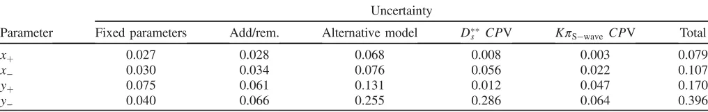
Model uncertainties arise due to fixing parameters in the amplitude model (denoted “fixed pars” in TableVI), the addition or removal of marginal components, namely the Kð1410Þ0, Kð1680Þ0, D1ð2760Þ−, D3ð2760Þ−, and

D_s2ð2573Þþ resonances, in the Dalitz plot fit (add/rem.), and the use of alternative models for the Kþπ− S-wave and Dπ− nonresonant amplitudes (alt. mod.); all of these are evaluated as in Ref. [27]. The possibilities of

CP violation associated with the D_s1ð2700Þþ amplitude

(Ds CPV), and of independent CP violation param-eters in the two components of the Kþπ− S-wave amplitude [50] (KπS−wave CPV), are also accounted for.

The largest source of uncertainty in this category arises from changing the description of the Kþπ− S-wave. Other possible sources of systematic uncertainty, such as production asymmetry [51] or CP violation in the

D→KþK− and πþπ− decays [52–54], are found to be negligible.

The total uncertainties are obtained by combining all sources in quadrature. The leading sources of systematic uncertainty are expected to be reducible with larger data samples.

VII. RESULTS AND SUMMARY

The DPs for candidates in the Bcandidate mass signal region in the D→KþK− and πþπ− samples are shown separately forB¯0andB0candidates in Fig.7. Projections of the fit results onto mðDπÞ, mðKπÞ, and mðDKÞ for the TABLE V. Experimental systematic uncertainties.

Parameter

Uncertainty

S=B ϵ BDP Fit bias Basym. BDP asym. ϵasym. Total

xþ 0.010 0.035 0.046 0.021 0.007 0.049 0.000 0.079

x− 0.026 0.028 0.063 0.019 0.010 0.045 0.001 0.089

yþ 0.019 0.042 0.122 0.066 0.017 0.027 0.000 0.149

y− 0.024 0.022 0.054 0.035 0.018 0.071 0.000 0.103

TABLE VI. Model uncertainties.

Parameter

Uncertainty

Fixed parameters Add/rem. Alternative model Ds CPV KπS−wave CPV Total

xþ 0.027 0.028 0.068 0.008 0.003 0.079

x− 0.030 0.034 0.076 0.056 0.022 0.107

yþ 0.075 0.061 0.131 0.012 0.047 0.170

y− 0.040 0.066 0.255 0.286 0.064 0.396

] 4 c / 2 ) [GeV

+ π

D ( 2 m

5 10 15 20

]

4

c

/

2

) [GeV

+

π

−

K

(

2

m

0 2 4 6 8 10 12

+ π − K D → 0 B

LHCb (a)

] 4 c / 2 ) [GeV

− π

D ( 2 m

5 10 15 20

]

4_c

/

2

) [GeV

−

π

+

K

(

2

m

0 2 4 6 8 10 12

− π + K D → 0 B

LHCb (b)

D→KþK−andπþπ−samples are shown separately forB¯0

and B0 candidates in Fig. 8. No significant CP violation effect is seen.

The results, with statistical uncertainties only, for the complex coefficients cj are given in Table VII. Due to the changes in the selection requirements, the overlap between the D→Kþπ− sample and the data set used in Ref.[27]is only around 60%, and the results are found to be consistent.

The results for the CPviolation parameters associated with the B0→DKð892Þ0 decay are

xþ¼0.040.160.11;

yþ¼−0.470.280.22;

x−¼−0.020.130.14; y−¼−0.350.260.41;

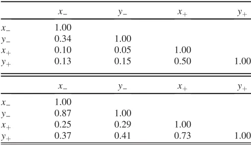
where the uncertainties are statistical and systematic. The statistical and systematic correlation matrices are given in TableVIII. The results forðxþ; yþÞandðx−; y−Þare shown

as contours in Fig.9.

] 2 c ) [GeV/ + π D ( m

2 3 4

)

2

c

Weighted candidates / (60 MeV/

0 5 10 15 20 25 30 + π − K D → 0 B

LHCb (a)

] 2 c ) [GeV/ − π D ( m

2 3 4

)

2

c

Weighted candidates / (60 MeV/

0 5 10 15 20 25 30 − π + K D → 0 B

LHCb (b)

] 2 c ) [GeV/ + π − K ( m

1 2 3

)

2

c

Weighted candidates / (60 MeV/

0 5 10 15 20 25 30 35 + π − K D → 0 B

LHCb (c)

] 2 c ) [GeV/ − π + K ( m

1 2 3

)

2

c

Weighted candidates / (60 MeV/

0 5 10 15 20 25 30 35 − π + K D → 0 B

LHCb (d)

] 2 c ) [GeV/ − K D ( m

3 4 5

)

2

c

Weighted candidates / (60 MeV/

0 5 10 15 20 25 30 35 + π − K D → 0 B

LHCb (e)

] 2 c ) [GeV/ + K D ( m

3 4 5

)

2

c

Weighted candidates / (60 MeV/

0 5 10 15 20 25 30 35 − π + K D → 0 B

LHCb (f)

Data Total fit K*(892)0 K*(1410)0 S-wave

π

K K*₂(1430)0 D₀*(2400)− D*₂(2460)− S-wave

π

D Dπ P-wave D_s1*(2700)+ D*−

Comb. bkgd. Mis-ID bkgd. Bs0 bkgd.

FIG. 8. Projections of the D→KþK− and πþπ− samples and the fit result onto (a),(b) mðDπ∓Þ, (c),(d)mðKπ∓Þ, and (e),(f) mðDKÞfor (a),(c),(e)B¯0and (b),(d),(f)B0candidates. The data and the fit results in each NN output bin have been weighted according toS=ðSþBÞand combined. The components are described in the legend.

The GammaCombo package [55] is used to evaluate

constraints from these results on γ and the hadronic parameters rB and δB associated with the B0→

DKð892Þ0 decay. A frequentist treatment referred to as the“plug-in”method, described in Refs. [56–59], is used. Figure10shows the results of likelihood scans for γ, rB, and δ_B. Figure 11 shows the two-dimensional 68% con-fidence level for each pair of observables from γ,rB, and δB. No value of γ is excluded at 95% confidence level (C.L.); the world-average value for γ [60,61] has a C.L. of 0.85.

TheB0→DKð892Þ0decay can also be used to deter-mine parameters sensitive to γ with a quasi-two-body approach, as has been done with D→KþK−, πþπ−

[62], Kπ∓, Kπ∓π0, Kπ∓πþπ− [62–64] and D→ K0_Sπþπ− decays [65–68]. In the quasi-two-body analysis, the results depend on the effective hadronic parametersκ, ¯

rB, and δ¯B, which are, respectively, the coherence factor

and the relative magnitude and strong phase of theVuband

Vcbamplitudes averaged over the selected region of phase space[17]. Precise definitions are given in the Appendix. These parameters are calculated from the models forVcb andVub amplitudes obtained from the fit for theKð892Þ0 selection regionjmðKþπ−Þ−mKð892Þ0j<50MeV=c2and

jcosθ_K0j>0.4, wherem_Kð892Þ0 is the known value of the

Kð892Þ0mass[37]andθ_K0 is theK0helicity angle, i.e. the angle between theKþandDdirections in theKþπ−rest frame. To reduce correlations with the values for rB and δ_B determined from the DP analysis, the quantities

¯

RB¼r¯B=rB and Δδ¯B¼δ¯B−δB are calculated. The results are

κ¼0.958₋þ0_0..₀₁₀005þ0_−0..₀₄₅002;

¯

RB¼1.02−þ00..01030.06; Δδ¯B¼0.02þ0−0..02030.11;

where the uncertainties are statistical and systematic and are evaluated as described in the Appendix.

In summary, a data sample corresponding to3.0fb−1of

ppcollisions collected with the LHCb detector has been used to measure, for the first time, parameters sensitive to the angle γ from a Dalitz plot analysis of B0→DKþπ−

decays. No significant CP violation effect is seen. The results are consistent with, and supersede, the results for AKK;_d ππ and RKK;_d ππ from Ref. [62]. Parameters that are needed to determine γ from quasi-two-body analyses of B0→DKð892Þ0 decays are measured. These results can be combined with current and future measurements with the B0→DKð892Þ0 channel to obtain stronger constraints onγ.

TABLE VII. Results for the complex coefficientscjfrom the fit to data. Uncertainties are statistical only. All reported quantities are unconstrained in the fit, except that the D2ð2460Þ− compo-nent is fixed as a reference amplitude, and the magnitude of the Ds1ð2700Þþcomponent is constrained. TheKþπ−S-wave is the coherent sum of theK0ð1430Þ0and the nonresonantKπS-wave component[50].

Resonance Real part Imaginary part

Kð892Þ0 −0.070.10 −1.190.04 Kð1410Þ0 0.160.04 0.210.06 K₀ð1430Þ0 0.400.08 0.670.06 NonresonantKπ S-wave 0.370.07 0.690.07 K₂ð1430Þ0 −0.010.06 −0.480.04 D0ð2400Þ− −1.100.05 −0.180.07

D₂ð2460Þ− 1.00 0.00

NonresonantDπ S-wave −0.440.06 0.020.07 NonresonantDπ P-wave −0.610.05 −0.080.06 Ds1ð2700Þþ 0.570.05 −0.090.19

±

x

-1 -0.5 0 0.5 1

±

y

-1 -0.5 0 0.5 1

LHCb

FIG. 9. Contours at 68% C.L. for the (blue)ðxþ; yþÞand (red)

ðx−; y−Þparameters associated with theB0→DKð892Þ0decay, with statistical uncertainties only. The central values are marked by a circle and a cross, respectively.

TABLE VIII. Correlation matrices associated with the (left) statistical and (right) systematic uncertainties of theCPviolation parameters associated with theB0→DKð892Þ0 decay.

x− y− xþ yþ

x− 1.00

y− 0.34 1.00

xþ 0.10 0.05 1.00

yþ 0.13 0.15 0.50 1.00

x− y− xþ yþ

x− 1.00

y− 0.87 1.00

xþ 0.25 0.29 1.00

ACKNOWLEDGMENTS

We express our gratitude to our colleagues in the CERN accelerator departments for the excellent performance of the LHC. We thank the technical and administrative staff at the LHCb institutes. We acknowledge support from CERN and from the national agencies: CAPES, CNPq, FAPERJ and FINEP (Brazil); NSFC (China); CNRS/IN2P3 (France); BMBF, DFG and MPG (Germany); INFN (Italy); FOM and NWO (The Netherlands); MNiSW and

NCN (Poland); MEN/IFA (Romania); MinES and FANO (Russia); MinECo (Spain); SNSF and SER (Switzerland); NASU (Ukraine); STFC (United Kingdom); NSF (USA). We acknowledge the computing resources that are provided by CERN, IN2P3 (France), KIT and DESY (Germany), INFN (Italy), SURF (The Netherlands), PIC (Spain), GridPP (United Kingdom), RRCKI and Yandex LLC (Russia), CSCS (Switzerland), IFIN-HH (Romania), CBPF (Brazil), PL-GRID (Poland) and OSC (USA). We ]

°

[

γ

1-CL

0 0.2 0.4 0.6 0.8 1

50 100 150

68.3%

95.5%

LHCb

B

r

0.2 0.4 0.6 0.8

1-CL

0 0.2 0.4 0.6 0.8 1

68.3%

95.5%

LHCb

]

°

[

B

δ

1-CL

0 0.2 0.4 0.6 0.8 1

100

− 0 100

68.3%

95.5%

LHCb

(b) (a)

(c)

FIG. 10. Results of likelihood scans for (a)γ, (b)rB, and (c)δB.

]

°

[

γ

B

r

50 100 150

0 0.2 0.4 0.6 0.8 1

LHCb

]

°

[

γ

]

°

[_B

δ

50 100 150

100

−

0

100 LHCb

B

r

]

°

[_B

δ

0.2 0.4 0.6 0.8

100

−

0

100 LHCb

(a) (b)

(c)

FIG. 11. Confidence level contours for (a)γandrB, (b)γandδB, and (c)rBandδB. The shaded regions are allowed at 68% C.L.

are indebted to the communities behind the multiple open source software packages on which we depend. Individual groups or members have received support from AvH Foundation (Germany), EPLANET, Marie Skł odowska-Curie Actions and ERC (European Union), Conseil Général de Haute-Savoie, Labex ENIGMASS and OCEVU, Région Auvergne (France), RFBR and Yandex LLC (Russia), GVA, XuntaGal and GENCAT (Spain), The Royal Society, Royal Commission for the Exhibition of 1851 and the Leverhulme Trust (United Kingdom).

APPENDIX: QUASI-TWO-BODY PARAMETERS

In the quasi-two-body analyses of B0→DKð892Þ0

decays, the following parameters are defined [17]:

κ¼

R

jA_{ffiffiffiffiffiffiffiffiffiffiffiffiffiffiffiffiffiffiffiffiffiffiffiffiffiffiffiffiffiffiffiffiffiffiffiffiffiffiffiffiffiffiffiffiffiffiffiffiffiffiffiffiffiffiffiffi}cbðpÞAubðpÞjexp½iδðpÞdp R

jAcbðpÞj2dp R

jAubðpÞj2dp

q ; ðA1Þ

¯

rB ¼

ffiffiffiffiffiffiffiffiffiffiffiffiffiffiffiffiffiffiffiffiffiffiffiffiffiffiffiffi R

jAubðpÞj2dp R

jAcbðpÞj2dp s

; ðA2Þ

¯ δB¼arg

0 B @ R

j_{ffiffiffiffiffiffiffiffiffiffiffiffiffiffiffiffiffiffiffiffiffiffiffiffiffiffiffiffiffiffiffiffiffiffiffiffiffiffiffiffiffiffiffiffiffiffiffiffiffiffiffiffiffiffiffiffi}AcbðpÞAubðpÞjexp½iδðpÞdp R

jAcbðpÞj2dp R

jAubðpÞj2dp q

1 C

A; ðA3Þ

where all the integrations are over the part of the phase space p inside the used Kð892Þ0 selection window. In

these equations,jAcbðpÞjandjAubðpÞjrefer to the magni-tudes of the totalVcbandVubamplitudes, andδðpÞis their relative strong phase. In terms of the parameters used in this analysis,

jAcbðpÞj ¼

X

j

cjFjðpÞ

; ðA4Þ

jAubðpÞj ¼

X

j

cjrB;jexp½iδB;jFjðpÞ

; ðA5Þ

δðpÞ ¼arg P

jcjrB;j_Pexp½iδB;jFjðpÞ jcjFjðpÞ

; ðA6Þ

where the rB;j, δB;j values are allowed to differ for each

Kþπ− resonance, and rB;j¼0 for Dπ− resonances. [The

rB, δB notation without thejsubscript is retained for the parameters associated with the B0→DKð892Þ0 decay.] In the limit that there is no amplitude (either resonant or nonresonant) contributing within the Kð892Þ0 selection window other than those associated with the B0→ DKð892Þ0 decay, one finds jAubðpÞj→rBjAcbðpÞj and δðpÞ→δB, and hence κ→1, r¯B→rB, and δ¯B→δB. In order to reduce correlations between r¯B and rB and between δ¯_B and δ_B, it is convenient to introduce the parameters

κ

0.9 0.92 0.94 0.96 0.98 1

Probability

0 0.02 0.04 0.06 0.08 0.1 0.12 0.14 0.16 0.18 0.2 0.22

(a) LHCb

B

R

0.9 1 1.1 1.2

Probability

0 0.05 0.1 0.15 0.2 0.25

(b) LHCb

B

δ Δ

-0.1 -0.05 0 0.05 0.1

Probability

0 0.02 0.04 0.06 0.08 0.1 0.12 0.14

(c) LHCb

¯

RB ¼ ¯

rB

rB

; ðA7Þ

Δδ¯B¼δ¯B−δB; ðA8Þ

which are obtained by replacing allrB;jbyrB;j=rB and all δB;j by δB;j−δB in Eqs.(A4)–(A6).

These quantities are determined from the results of the Dalitz plot analysis. An alternative fit is performed with x;jþiy;j, defined in Eq. (2), replaced by

rB;jexp½iðδB;jγÞ. The results of this fit are consistent with the values forγ,rB, andδBobtained from the fittedx and y, and are used to evaluate jAcbðpÞj, jAubðpÞj and δðpÞ at many points inside the selection window and thereby to determine κ, R¯B, and Δδ¯B. The procedure is repeated many times with both Vcb and Vub amplitude model parameters varied within their statistical

uncertainties from the fit, leading to the distributions shown in Fig.12. Since the transformations from the fitted model parameters to the quasi-two-body parameters are highly nonlinear, the reported central values correspond to the peak positions of these distributions, while positive and negative uncertainties are obtained by incrementally including the most probable values until 68% of all entries are covered.

Sources of systematic uncertainty are accounted for by evaluating their effects on the quasi-two-body parameters. The dominant sources are from the use of an alternative description of the Kþπ− S-wave, and from changing the treatment ofCP violation in theD_s1ð2700Þþ component and theKþπ− S-wave. Most systematic uncertainties are symmetrized for consistency with the rest of the analysis, but asymmetric systematic uncertainties are reported onκ since this quantity is≤1 by definition.

[1] N. Cabibbo, Unitary Symmetry and Leptonic Decays,Phys. Rev. Lett.10, 531 (1963).

[2] M. Kobayashi and T. Maskawa, CP violation in the renormalizable theory of weak interaction, Prog. Theor. Phys.49, 652 (1973).

[3] L. Wolfenstein, Parametrization of the Kobayashi-Maskawa Matrix,Phys. Rev. Lett.51, 1945 (1983).

[4] C. Jarlskog, Commutator of the Quark Mass Matrices in the Standard Electroweak Model and a Measure of MaximalCP Violation,Phys. Rev. Lett.55, 1039 (1985).

[5] A. J. Buras, M. E. Lautenbacher, and G. Ostermaier, Waiting for the top quark mass,Kþ→πþνν¯,B0s–B¯0smixing andCP asymmetries inB decays,Phys. Rev. D50, 3433 (1994).

[6] A. Riotto and M. Trodden, Recent progress in baryogenesis, Annu. Rev. Nucl. Part. Sci.49, 35 (1999).

[7] M. Gronau and D. London, How to determine all the angles of the unitarity triangle from B0→DK0S and B0s →Dϕ, Phys. Lett. B253, 483 (1991).

[8] M. Gronau and D. Wyler, On determining a weak phase from chargedBdecay asymmetries,Phys. Lett. B265, 172 (1991).

[9] D. Atwood, I. Dunietz, and A. Soni, EnhancedCPViolation withB→KD0ðD¯0ÞModes and Extraction of the Cabibbo-Kobayashi-Maskawa Angle γ, Phys. Rev. Lett. 78, 3257 (1997).

[10] D. Atwood, I. Dunietz, and A. Soni, Improved methods for observingCPviolation inB→KD and measuring the CKM phaseγ,Phys. Rev. D63, 036005 (2001).

[11] J. Brod and J. Zupan, The ultimate theoretical error on γ from B→DK decays, J. High Energy Phys. 01 (2014) 051.

[12] T. Gershon, On the measurement of the unitarity triangle angleγfromB0→DK0decays,Phys. Rev. D79, 051301 (2009).

[13] T. Gershon and M. Williams, Prospects for the measurement of the unitarity triangle angleγfromB0→DKþπ−decays, Phys. Rev. D80, 092002 (2009).

[14] R. H. Dalitz, On the analysis ofτ-meson data and the nature of theτ-meson,Philos. Mag. Ser. 544, 1068 (1953). [15] I. I. Bigi and A. I. Sanda, On direct CP violation in

B→ð−ÞD 0

Kπ’s versus B¯ →ð−ÞD 0

¯

Kπ’s decays, Phys. Lett. B

211, 213 (1988).

[16] I. Dunietz,CPviolation with self-taggingB0modes,Phys. Lett. B270, 75 (1991).

[17] M. Gronau, Improving bounds on γ in B→DK and B;0_→DX;0

s ,Phys. Lett. B557, 198 (2003).

[18] A. A. Alves, Jr. et al. (LHCb Collaboration), The LHCb detector at the LHC, J. Instrum.3, S08005 (2008). [19] R. Aaij et al. (LHCb Collaboration), LHCb detector

performance,Int. J. Mod. Phys. A30, 1530022 (2015). [20] A. Puig, CERN Report No. LHCb-PUB-2014-046, 2014. [21] T. Sjöstrand, S. Mrenna, and P. Skands, A brief introduction

to PYTHIA 8.1,Comput. Phys. Commun.178, 852 (2008); PYTHIA 6.4 physics and manual,J. High Energy Phys. 05 (2006) 026.

[22] I. Belyaev et al., Handling of the generation of primary events in Gauss, the LHCb simulation framework,J. Phys. Conf. Ser.331, 032047 (2011).

[23] D. J. Lange, The EvtGen particle decay simulation package, Nucl. Instrum. Methods Phys. Res., Sect. A462, 152 (2001). [24] P. Golonka and Z. Was, PHOTOS Monte Carlo: A precision tool for QED corrections inZandWdecays,Eur. Phys. J. C

45, 97 (2006).

[25] J. Allisonet al. (Geant4 Collaboration), Geant4 develop-ments and applications, IEEE Trans. Nucl. Sci. 53, 270 (2006); S. Agostinelliet al.(Geant4 Collaboration), Geant4: A simulation toolkit,Nucl. Instrum. Methods Phys. Res., Sect. A506, 250 (2003).

[26] M. Clemencic, G. Corti, S. Easo, C. R. Jones, S. Miglioranzi, M. Pappagallo, and P. Robbe, The LHCb simulation application, Gauss: Design, evolution and experience, J. Phys. Conf. Ser.331, 032023 (2011).

[27] R. Aaij et al. (LHCb Collaboration), Amplitude analysis of B0→D¯0Kþπ− decays, Phys. Rev. D 92, 012012 (2015).

[28] R. Aaij et al. (LHCb Collaboration), Observation of the decayB0s →D¯0ϕ,Phys. Lett. B727, 403 (2013).

[29] R. Aaijet al.(LHCb Collaboration), Observation ofB0s–B¯0s mixing and measurement of mixing frequencies using semileptonicBdecays,Eur. Phys. J. C73, 2655 (2013). [30] R. Aaijet al.(LHCb Collaboration), First evidence for the

annihilation decay modeBþ→Dþsϕ,J. High Energy Phys. 02 (2013) 043.

[31] R. Aaijet al.(LHCb Collaboration), First observations of ¯

B0s →DþD−,DþsD− andD0D¯0 decays,Phys. Rev. D 87, 092007 (2013).

[32] M. Feindt and U. Kerzel, The NeuroBayes neural network package,Nucl. Instrum. Methods Phys. Res., Sect. A559, 190 (2006).

[33] M. Pivk and F. R. Le Diberder, sPlot: A statistical tool to unfold data distributions, Nucl. Instrum. Methods Phys. Res., Sect. A555, 356 (2005).

[34] R. Aaij et al. (LHCb Collaboration), Search for the decay B0s →D¯0f0ð980Þ, J. High Energy Phys. 08 (2015) 005.

[35] R. Aaijet al.(LHCb Collaboration), First observation of the rareBþ→DþKþπ− decay,Phys. Rev. D 93, 051101(R) (2016).

[36] T. Skwarnicki, Ph.D. thesis, Institute of Nuclear Physics, Krakow, 1986; DESY Report No. DESY-F31-86-02, 1986. [37] K. A. Oliveet al.(Particle Data Group), Review of particle physics,Chin. Phys. C38, 090001 (2014), and 2015 update. [38] R. Aaijet al.(LHCb Collaboration), Observation of over-lapping spin-1 and spin-3 D¯0K− resonances at mass 2.86GeV=c2,Phys. Rev. Lett.113, 162001 (2014). [39] R. Aaij et al. (LHCb Collaboration), Dalitz plot analysis

of B0s→D¯0K−πþ decays, Phys. Rev. D 90, 072003 (2014).

[40] R. Aaij et al. (LHCb Collaboration), Dalitz plot analysis of B0→D¯0πþπ− decays, Phys. Rev. D 92, 032002 (2015).

[41] A. Kuzmin et al. (Belle Collaboration), Study of B¯0→ D0πþπ− decays,Phys. Rev. D76, 012006 (2007). [42] K. Abe et al. (Belle Collaboration), Study of B0→

¯

DðÞ0πþπ−decays,arXiv:hep-ex/0412072.

[43] R. Aaijet al.(LHCb Collaboration), Observation ofB0→ ¯

D0KþK− and Evidence for B0s →D¯0KþK−, Phys. Rev. Lett.109, 131801 (2012).

[44] R. Aaijet al.(LHCb Collaboration), Study of beauty baryon decays toD0ph− andΛþ_ch−final states,Phys. Rev. D89, 032001 (2014).

[45] M. Adinolfiet al., Performance of the LHCb RICH detector at the LHC,Eur. Phys. J. C73, 2431 (2013).

[46] E. Ben-Haim, R. Brun, B. Echenard, and T. E. Latham, JFIT: A framework to obtain combined experimental results through joint fits,arXiv:1409.5080.

[47] Lauraþ þDalitz plot fitting package,http://laura.hepforge .org/, University of Warwick.

[48] R. Aaij et al. (LHCb Collaboration), Study ofDJ meson decays to Dþπ−, D0πþ and Dþπ− final states in pp collisions,J. High Energy Phys. 09 (2013) 145.

[49] J. P. Leeset al.(BABARCollaboration), Dalitz plot analyses ofB0→D−D0KþandBþ→D¯0D0Kþdecays,Phys. Rev. D91, 052002 (2015).

[50] D. Aston et al.(LASS Collaboration), A study of K−πþ scattering in the reaction K−p→K−πþn at 11GeV=c, Nucl. Phys.B296, 493 (1988).

[51] R. Aaijet al. (LHCb Collaboration), Measurement of the ¯

B0–B0andB¯0s–B0s production asymmetries inppcollisions atpffiffiffis¼7TeV,Phys. Lett. B739, 218 (2014).

[52] Y. Amhiset al.(Heavy Flavor Averaging Group), Averages ofb-hadron,c-hadron, andτ-lepton properties as of summer 2014,arXiv:1412.7515, updated results and plots available at http://www.slac.stanford.edu/xorg/hfag/.

[53] R. Aaij et al. (LHCb Collaboration), Measurement of indirect CP asymmetries in D0→K−Kþ and D0→

π−_πþ_{decays,J. High Energy Phys. 04 (2015) 043.}

[54] R. Aaij et al. (LHCb Collaboration), Measurement of the difference of time-integrated CP asymmetries in D0→K−Kþ and D0→π−πþ decays, Phys. Rev. Lett.

116, 191601 (2016).

[55] GammaCombo framework for combinations of measure-ments and computation of confidence intervals, http:// gammacombo.hepforge.org/, CERN.

[56] R. Aaijet al.(LHCb Collaboration), A measurement of the CKM angleγfrom a combination ofB→Dhanalyses, Phys. Lett. B726, 151 (2013).

[57] LHCb Collaboration, Report No. LHCb-CONF-2014-004, 2014.

[58] LHCb Collaboration, CERN Report No. LHCb-CONF-2016-001, 2016.

[59] B. Sen, M. Walker, and M. Woodroofe, On the unified method with nuisance parameters, Statistica Sinica19, 301 (2009). [60] J. Charles, A. Höcker, H. Lacker, S. Laplace, F. R. Le

Diberder, J. Malclés, J. Ocariz, M. Pivk, and L. Roos (CKMfitter Group), CP violation and the CKM matrix: Assessing the impact of the asymmetric B factories, Eur. Phys. J. C41, 1 (2005).

[61] M. Bona et al. (UTfit Collaboration), The 2004 UTfit Collaboration report on the status of the unitarity triangle in the standard model, J. High Energy Phys. 07 (2005) 028.

[62] R. Aaijet al.(LHCb Collaboration), Measurement ofCP violation parameters inB0→DK0 decays, Phys. Rev. D

90, 112002 (2014).

[63] B. Aubertet al.(BABARCollaboration), Search forb→u transitions inB0→D0K0decays,Phys. Rev. D80, 031102 (2009).

[64] K. Negishiet al.(Belle Collaboration), Search for the decay B0→DK0 followed by D→K−πþ, Phys. Rev. D 86, 011101 (2012).

[65] B. Aubertet al.(BABARCollaboration), Constraints on the CKM angle γ in B0→D¯0K0 and B0→D0K0 from a Dalitz analysis ofD0andD¯0decays toK0Sπþπ−,Phys. Rev. D79, 072003 (2009).

[67] R. Aaij et al. (LHCb Collaboration), Model-independent measurement of the CKM angleγusingB0→DK0decays withD→K0Sπþπ− andK0SKþK−,arXiv:1604.01525.

[68] R. Aaijet al. (LHCb Collaboration), Measurement of the CKM angleγusingB0→DK0withD→K0Sπþπ−decays, arXiv:1605.01082.

R. Aaij,39C. Abellán Beteta,41B. Adeva,38M. Adinolfi,47A. Affolder,53Z. Ajaltouni,5S. Akar,6J. Albrecht,10F. Alessio,39 M. Alexander,52S. Ali,42G. Alkhazov,31P. Alvarez Cartelle,54A. A. Alves Jr.,58S. Amato,2S. Amerio,23Y. Amhis,7

L. An,3,40L. Anderlini,18G. Andreassi,40M. Andreotti,17,a J. E. Andrews,59R. B. Appleby,55O. Aquines Gutierrez,11 F. Archilli,39P. d’Argent,12A. Artamonov,36M. Artuso,60E. Aslanides,6G. Auriemma,26,bM. Baalouch,5S. Bachmann,12

J. J. Back,49A. Badalov,37C. Baesso,61W. Baldini,17,39R. J. Barlow,55C. Barschel,39S. Barsuk,7 W. Barter,39 V. Batozskaya,29V. Battista,40A. Bay,40L. Beaucourt,4J. Beddow,52F. Bedeschi,24I. Bediaga,1L. J. Bel,42V. Bellee,40

N. Belloli,21,cI. Belyaev,32E. Ben-Haim,8G. Bencivenni,19S. Benson,39J. Benton,47 A. Berezhnoy,33R. Bernet,41 A. Bertolin,23F. Betti,15M.-O. Bettler,39M. van Beuzekom,42S. Bifani,46P. Billoir,8T. Bird,55A. Birnkraut,10A. Bizzeti,18,d T. Blake,49F. Blanc,40J. Blouw,11S. Blusk,60V. Bocci,26A. Bondar,35N. Bondar,31,39W. Bonivento,16A. Borgheresi,21,c

S. Borghi,55M. Borisyak,67M. Borsato,38 T. J. V. Bowcock,53E. Bowen,41C. Bozzi,17,39S. Braun,12M. Britsch,12 T. Britton,60J. Brodzicka,55N. H. Brook,47E. Buchanan,47C. Burr,55A. Bursche,2 J. Buytaert,39S. Cadeddu,16 R. Calabrese,17,a M. Calvi,21,cM. Calvo Gomez,37,e P. Campana,19D. Campora Perez,39L. Capriotti,55A. Carbone,15,f G. Carboni,25,gR. Cardinale,20,hA. Cardini,16P. Carniti,21,cL. Carson,51K. Carvalho Akiba,2 G. Casse,53L. Cassina,21,c

L. Castillo Garcia,40M. Cattaneo,39 Ch. Cauet,10G. Cavallero,20R. Cenci,24,iM. Charles,8 Ph. Charpentier,39 M. Chefdeville,4 S. Chen,55S.-F. Cheung,56N. Chiapolini,41M. Chrzaszcz,41,27 X. Cid Vidal,39G. Ciezarek,42 P. E. L. Clarke,51M. Clemencic,39H. V. Cliff,48J. Closier,39V. Coco,39J. Cogan,6 E. Cogneras,5 V. Cogoni,16,j L. Cojocariu,30G. Collazuol,23,kP. Collins,39A. Comerma-Montells,12A. Contu,39A. Cook,47 M. Coombes,47 S. Coquereau,8G. Corti,39M. Corvo,17,aB. Couturier,39G. A. Cowan,51D. C. Craik,51A. Crocombe,49M. Cruz Torres,61

S. Cunliffe,54R. Currie,54C. D’Ambrosio,39E. Dall’Occo,42J. Dalseno,47P. N. Y. David,42A. Davis,58

O. De Aguiar Francisco,2K. De Bruyn,6S. De Capua,55M. De Cian,12J. M. De Miranda,1L. De Paula,2P. De Simone,19 C.-T. Dean,52D. Decamp,4M. Deckenhoff,10L. Del Buono,8N. Déléage,4M. Demmer,10D. Derkach,67O. Deschamps,5

F. Dettori,39B. Dey,22A. Di Canto,39F. Di Ruscio,25H. Dijkstra,39 S. Donleavy,53F. Dordei,39 M. Dorigo,40 A. Dosil Suárez,38A. Dovbnya,44K. Dreimanis,53L. Dufour,42G. Dujany,55K. Dungs,39P. Durante,39R. Dzhelyadin,36 A. Dziurda,27A. Dzyuba,31S. Easo,50,39U. Egede,54V. Egorychev,32S. Eidelman,35S. Eisenhardt,51U. Eitschberger,10 R. Ekelhof,10 L. Eklund,52I. El Rifai,5 Ch. Elsasser,41S. Ely,60S. Esen,12H. M. Evans,48T. Evans,56A. Falabella,15

C. Färber,39 N. Farley,46S. Farry,53R. Fay,53 D. Fazzini,21,c D. Ferguson,51V. Fernandez Albor,38F. Ferrari,15 F. Ferreira Rodrigues,1 M. Ferro-Luzzi,39S. Filippov,34M. Fiore,17,39,a M. Fiorini,17,aM. Firlej,28C. Fitzpatrick,40 T. Fiutowski,28F. Fleuret,7,lK. Fohl,39M. Fontana,16F. Fontanelli,20,hD. C. Forshaw,60R. Forty,39M. Frank,39C. Frei,39

M. Frosini,18J. Fu,22E. Furfaro,25,gA. Gallas Torreira,38D. Galli,15,f S. Gallorini,23S. Gambetta,51M. Gandelman,2 P. Gandini,56Y. Gao,3J. García Pardiñas,38J. Garra Tico,48L. Garrido,37D. Gascon,37C. Gaspar,39L. Gavardi,10 G. Gazzoni,5D. Gerick,12E. Gersabeck,12M. Gersabeck,55T. Gershon,49Ph. Ghez,4S. Gianì,40V. Gibson,48O. G. Girard,40

L. Giubega,30V. V. Gligorov,39C. Göbel,61D. Golubkov,32A. Golutvin,54,39A. Gomes,1,m C. Gotti,21,c M. Grabalosa Gándara,5R. Graciani Diaz,37L. A. Granado Cardoso,39E. Graugés,37E. Graverini,41G. Graziani,18 A. Grecu,30P. Griffith,46L. Grillo,12O. Grünberg,65B. Gui,60E. Gushchin,34Yu. Guz,36,39 T. Gys,39T. Hadavizadeh,56 C. Hadjivasiliou,60G. Haefeli,40C. Haen,39S. C. Haines,48S. Hall,54B. Hamilton,59X. Han,12S. Hansmann-Menzemer,12 N. Harnew,56S. T. Harnew,47J. Harrison,55J. He,39T. Head,40V. Heijne,42A. Heister,9 K. Hennessy,53P. Henrard,5 L. Henry,8J. A. Hernando Morata,38E. van Herwijnen,39M. Heß,65A. Hicheur,2D. Hill,56M. Hoballah,5C. Hombach,55

L. Hongming,40W. Hulsbergen,42T. Humair,54M. Hushchyn,67N. Hussain,56D. Hutchcroft,53M. Idzik,28P. Ilten,57 R. Jacobsson,39 A. Jaeger,12J. Jalocha,56 E. Jans,42A. Jawahery,59M. John,56D. Johnson,39C. R. Jones,48C. Joram,39 B. Jost,39N. Jurik,60S. Kandybei,44W. Kanso,6M. Karacson,39T. M. Karbach,39,†S. Karodia,52M. Kecke,12M. Kelsey,60 I. R. Kenyon,46M. Kenzie,39T. Ketel,43E. Khairullin,67B. Khanji,21,39,c C. Khurewathanakul,40T. Kirn,9S. Klaver,55

K. Klimaszewski,29O. Kochebina,7 M. Kolpin,12I. Komarov,40R. F. Koopman,43P. Koppenburg,42,39M. Kozeiha,5 L. Kravchuk,34K. Kreplin,12M. Kreps,49P. Krokovny,35F. Kruse,10W. Krzemien,29W. Kucewicz,27,nM. Kucharczyk,27

V. Kudryavtsev,35A. K. Kuonen,40K. Kurek,29T. Kvaratskheliya,32D. Lacarrere,39G. Lafferty,55,39A. Lai,16D. Lambert,51 G. Lanfranchi,19C. Langenbruch,49B. Langhans,39T. Latham,49C. Lazzeroni,46R. Le Gac,6J. van Leerdam,42J.-P. Lees,4

R. Lefèvre,5 A. Leflat,33,39 J. Lefrançois,7 E. Lemos Cid,38O. Leroy,6T. Lesiak,27B. Leverington,12Y. Li,7 T. Likhomanenko,67,66 M. Liles,53R. Lindner,39C. Linn,39F. Lionetto,41B. Liu,16X. Liu,3 D. Loh,49I. Longstaff,52

J. H. Lopes,2 D. Lucchesi,23,k M. Lucio Martinez,38H. Luo,51A. Lupato,23E. Luppi,17,a O. Lupton,56A. Lusiani,24 F. Machefert,7F. Maciuc,30O. Maev,31K. Maguire,55S. Malde,56A. Malinin,66G. Manca,7G. Mancinelli,6P. Manning,60 A. Mapelli,39J. Maratas,5J. F. Marchand,4U. Marconi,15C. Marin Benito,37P. Marino,24,39,iJ. Marks,12G. Martellotti,26

M. Martin,6 M. Martinelli,40D. Martinez Santos,38F. Martinez Vidal,68D. Martins Tostes,2 L. M. Massacrier,7 A. Massafferri,1 R. Matev,39A. Mathad,49Z. Mathe,39C. Matteuzzi,21 A. Mauri,41B. Maurin,40A. Mazurov,46 M. McCann,54J. McCarthy,46A. McNab,55 R. McNulty,13B. Meadows,58F. Meier,10M. Meissner,12D. Melnychuk,29

M. Merk,42A Merli,22,oE Michielin,23D. A. Milanes,64M.-N. Minard,4D. S. Mitzel,12J. Molina Rodriguez,61 I. A. Monroy,64 S. Monteil,5 M. Morandin,23P. Morawski,28A. Mordà,6M. J. Morello,24,iJ. Moron,28A. B. Morris,51 R. Mountain,60 F. Muheim,51 D. Müller,55J. Müller,10K. Müller,41V. Müller,10 M. Mussini,15B. Muster,40P. Naik,47 T. Nakada,40R. Nandakumar,50A. Nandi,56I. Nasteva,2M. Needham,51N. Neri,22S. Neubert,12N. Neufeld,39M. Neuner,12

A. D. Nguyen,40 C. Nguyen-Mau,40,p V. Niess,5 S. Nieswand,9 R. Niet,10N. Nikitin,33T. Nikodem,12A. Novoselov,36 D. P. O’Hanlon,49A. Oblakowska-Mucha,28V. Obraztsov,36 S. Ogilvy,52O. Okhrimenko,45R. Oldeman,16,48,j C. J. G. Onderwater,69B. Osorio Rodrigues,1 J. M. Otalora Goicochea,2 A. Otto,39P. Owen,54A. Oyanguren,68 A. Palano,14,q F. Palombo,22,o M. Palutan,19J. Panman,39 A. Papanestis,50M. Pappagallo,52L. L. Pappalardo,17,a C. Pappenheimer,58W. Parker,59C. Parkes,55G. Passaleva,18 G. D. Patel,53 M. Patel,54C. Patrignani,20,hA. Pearce,55,50 A. Pellegrino,42G. Penso,26,rM. Pepe Altarelli,39S. Perazzini,15,fP. Perret,5L. Pescatore,46K. Petridis,47A. Petrolini,20,h

M. Petruzzo,22E. Picatoste Olloqui,37B. Pietrzyk,4 M. Pikies,27D. Pinci,26A. Pistone,20A. Piucci,12S. Playfer,51 M. Plo Casasus,38T. Poikela,39F. Polci,8 A. Poluektov,49,35 I. Polyakov,32E. Polycarpo,2 A. Popov,36D. Popov,11,39

B. Popovici,30C. Potterat,2 E. Price,47J. D. Price,53J. Prisciandaro,38A. Pritchard,53C. Prouve,47V. Pugatch,45 A. Puig Navarro,40G. Punzi,24,sW. Qian,56R. Quagliani,7,47 B. Rachwal,27J. H. Rademacker,47M. Rama,24 M. Ramos Pernas,38M. S. Rangel,2 I. Raniuk,44G. Raven,43F. Redi,54S. Reichert,55A. C. dos Reis,1 V. Renaudin,7 S. Ricciardi,50S. Richards,47M. Rihl,39K. Rinnert,53,39V. Rives Molina,37P. Robbe,7,39A. B. Rodrigues,1E. Rodrigues,55

J. A. Rodriguez Lopez,64P. Rodriguez Perez,55A. Rogozhnikov,67S. Roiser,39V. Romanovsky,36A. Romero Vidal,38 J. W. Ronayne,13M. Rotondo,23T. Ruf,39P. Ruiz Valls,68J. J. Saborido Silva,38N. Sagidova,31B. Saitta,16,j V. Salustino Guimaraes,2 C. Sanchez Mayordomo,68B. Sanmartin Sedes,38 R. Santacesaria,26C. Santamarina Rios,38 M. Santimaria,19E. Santovetti,25,g A. Sarti,19,r C. Satriano,26,b A. Satta,25D. M. Saunders,47D. Savrina,32,33 S. Schael,9 M. Schiller,39H. Schindler,39M. Schlupp,10M. Schmelling,11T. Schmelzer,10B. Schmidt,39O. Schneider,40A. Schopper,39 M. Schubiger,40M.-H. Schune,7R. Schwemmer,39B. Sciascia,19A. Sciubba,26,rA. Semennikov,32A. Sergi,46N. Serra,41

J. Serrano,6 L. Sestini,23P. Seyfert,21M. Shapkin,36I. Shapoval,17,44,a Y. Shcheglov,31T. Shears,53L. Shekhtman,35 V. Shevchenko,66A. Shires,10 B. G. Siddi,17R. Silva Coutinho,41L. Silva de Oliveira,2 G. Simi,23,sM. Sirendi,48 N. Skidmore,47T. Skwarnicki,60E. Smith,54I. T. Smith,51J. Smith,48M. Smith,55 H. Snoek,42 M. D. Sokoloff,58,39 F. J. P. Soler,52F. Soomro,40D. Souza,47B. Souza De Paula,2 B. Spaan,10P. Spradlin,52S. Sridharan,39 F. Stagni,39 M. Stahl,12S. Stahl,39S. Stefkova,54O. Steinkamp,41O. Stenyakin,36S. Stevenson,56S. Stoica,30S. Stone,60B. Storaci,41 S. Stracka,24,iM. Straticiuc,30U. Straumann,41L. Sun,58W. Sutcliffe,54K. Swientek,28S. Swientek,10V. Syropoulos,43 M. Szczekowski,29T. Szumlak,28S. T’Jampens,4A. Tayduganov,6T. Tekampe,10G. Tellarini,17,aF. Teubert,39C. Thomas,56

E. Thomas,39J. van Tilburg,42 V. Tisserand,4 M. Tobin,40J. Todd,58S. Tolk,43L. Tomassetti,17,a D. Tonelli,39 S. Topp-Joergensen,56E. Tournefier,4 S. Tourneur,40K. Trabelsi,40M. Traill,52M. T. Tran,40M. Tresch,41A. Trisovic,39 A. Tsaregorodtsev,6P. Tsopelas,42N. Tuning,42,39A. Ukleja,29A. Ustyuzhanin,67,66U. Uwer,12C. Vacca,16,39,jV. Vagnoni,15 G. Valenti,15A. Vallier,7R. Vazquez Gomez,19P. Vazquez Regueiro,38C. Vázquez Sierra,38S. Vecchi,17M. van Veghel,43

J. J. Velthuis,47M. Veltri,18,tG. Veneziano,40M. Vesterinen,12B. Viaud,7 D. Vieira,2 M. Vieites Diaz,38

X. Vilasis-Cardona,37,eV. Volkov,33A. Vollhardt,41D. Voong,47A. Vorobyev,31V. Vorobyev,35C. Voß,65J. A. de Vries,42 R. Waldi,65C. Wallace,49R. Wallace,13J. Walsh,24J. Wang,60D. R. Ward,48N. K. Watson,46D. Websdale,54A. Weiden,41

M. Whitehead,39J. Wicht,49G. Wilkinson,56,39M. Wilkinson,60M. Williams,39M. P. Williams,46M. Williams,57 T. Williams,46 F. F. Wilson,50 J. Wimberley,59J. Wishahi,10W. Wislicki,29 M. Witek,27G. Wormser,7 S. A. Wotton,48

M. Zangoli,15M. Zavertyaev,11,uL. Zhang,3 Y. Zhang,3A. Zhelezov,12Y. Zheng,62A. Zhokhov,32L. Zhong,3 V. Zhukov,9 and S. Zucchelli15

(LHCb Collaboration)

1_{Centro Brasileiro de Pesquisas Físicas (CBPF), Rio de Janeiro, Brazil} 2

Universidade Federal do Rio de Janeiro (UFRJ), Rio de Janeiro, Brazil

3_{Center for High Energy Physics, Tsinghua University, Beijing, China} 4

LAPP, Université Savoie Mont-Blanc, CNRS/IN2P3, Annecy-Le-Vieux, France

5_{Clermont Université, Université Blaise Pascal, CNRS/IN2P3, LPC, Clermont-Ferrand, France} 6

CPPM, Aix-Marseille Université, CNRS/IN2P3, Marseille, France

7_{LAL, Université Paris-Sud, CNRS/IN2P3, Orsay, France} 8

LPNHE, Université Pierre et Marie Curie, Université Paris Diderot, CNRS/IN2P3, Paris, France

9

I. Physikalisches Institut, RWTH Aachen University, Aachen, Germany

10_{Fakultät Physik, Technische Universität Dortmund, Dortmund, Germany} 11

Max-Planck-Institut für Kernphysik (MPIK), Heidelberg, Germany

12_{Physikalisches Institut, Ruprecht-Karls-Universität Heidelberg, Heidelberg, Germany} 13

School of Physics, University College Dublin, Dublin, Ireland

14_{Sezione INFN di Bari, Bari, Italy} 15

Sezione INFN di Bologna, Bologna, Italy

16_{Sezione INFN di Cagliari, Cagliari, Italy} 17

Sezione INFN di Ferrara, Ferrara, Italy

18_{Sezione INFN di Firenze, Firenze, Italy} 19

Laboratori Nazionali dell’INFN di Frascati, Frascati, Italy

20_{Sezione INFN di Genova, Genova, Italy} 21

Sezione INFN di Milano Bicocca, Milano, Italy

22_{Sezione INFN di Milano, Milano, Italy} 23

Sezione INFN di Padova, Padova, Italy

24_{Sezione INFN di Pisa, Pisa, Italy} 25

Sezione INFN di Roma Tor Vergata, Roma, Italy

26_{Sezione INFN di Roma La Sapienza, Roma, Italy} 27

Henryk Niewodniczanski Institute of Nuclear Physics Polish Academy of Sciences, Kraków, Poland

28_{AGH—University of Science and Technology, Faculty of Physics and Applied Computer Science,}

Kraków, Poland

29_{National Center for Nuclear Research (NCBJ), Warsaw, Poland} 30

Horia Hulubei National Institute of Physics and Nuclear Engineering, Bucharest-Magurele, Romania

31_{Petersburg Nuclear Physics Institute (PNPI), Gatchina, Russia} 32

Institute of Theoretical and Experimental Physics (ITEP), Moscow, Russia

33_{Institute of Nuclear Physics, Moscow State University (SINP MSU), Moscow, Russia} 34

Institute for Nuclear Research of the Russian Academy of Sciences (INR RAN), Moscow, Russia

35_{Budker Institute of Nuclear Physics (SB RAS) and Novosibirsk State University, Novosibirsk, Russia} 36

Institute for High Energy Physics (IHEP), Protvino, Russia

37_{Universitat de Barcelona, Barcelona, Spain} 38

Universidad de Santiago de Compostela, Santiago de Compostela, Spain

39_{European Organization for Nuclear Research (CERN), Geneva, Switzerland} 40

Ecole Polytechnique Fédérale de Lausanne (EPFL), Lausanne, Switzerland

41_{Physik-Institut, Universität Zürich, Zürich, Switzerland} 42

Nikhef National Institute for Subatomic Physics, Amsterdam, The Netherlands

43_{Nikhef National Institute for Subatomic Physics and VU University Amsterdam,}

Amsterdam, The Netherlands

44_{NSC Kharkiv Institute of Physics and Technology (NSC KIPT), Kharkiv, Ukraine} 45

Institute for Nuclear Research of the National Academy of Sciences (KINR), Kyiv, Ukraine

46_{University of Birmingham, Birmingham, United Kingdom} 47

H.H. Wills Physics Laboratory, University of Bristol, Bristol, United Kingdom

48_{Cavendish Laboratory, University of Cambridge, Cambridge, United Kingdom} 49

Department of Physics, University of Warwick, Coventry, United Kingdom

50_{STFC Rutherford Appleton Laboratory, Didcot, United Kingdom} 51

School of Physics and Astronomy, University of Edinburgh, Edinburgh, United Kingdom