Modelling regulation of vascular tone following muscle contraction: model development, validation and global sensitivity analysis

This is a repository copy of

Modelling regulation of vascular tone following muscle

contraction: model development, validation and global sensitivity analysis

.

White Rose Research Online URL for this paper:

http://eprints.whiterose.ac.uk/117210/

Version: Accepted Version

Article:

Keijsers, J., Leguy, C., Narracott, A. orcid.org/0000-0002-3068-6192 et al. (3 more

authors) (2017) Modelling regulation of vascular tone following muscle contraction: model

development, validation and global sensitivity analysis. Journal of Computational Science.

ISSN 1877-7503

https://doi.org/10.1016/j.jocs.2017.04.007

Article available under the terms of the CC-BY-NC-ND licence

(https://creativecommons.org/licenses/by-nc-nd/4.0/).

eprints@whiterose.ac.uk https://eprints.whiterose.ac.uk/ Reuse

This article is distributed under the terms of the Creative Commons Attribution-NonCommercial-NoDerivs (CC BY-NC-ND) licence. This licence only allows you to download this work and share it with others as long as you credit the authors, but you can’t change the article in any way or use it commercially. More

information and the full terms of the licence here: https://creativecommons.org/licenses/

Takedown

If you consider content in White Rose Research Online to be in breach of UK law, please notify us by

Authors version; accepted for publication in Journal of Computational Science on April 23, 2017

Modeling regulation of vascular tone

following muscle contraction:

model development, validation and global

sensitivity analysis

J.M.T. Keijsers1,2,∗

, C.A.D. Leguy2

, A.J. Narracott3,4

, J. Rittweger2

, F.N. van de Vosse1

and W. Huberts5

1

Department of Biomedical Engineering, Eindhoven University of Technology, Eindhoven, The Netherlands

2

Institute of Aerospace Medicine, German Aerospace Center, Cologne, Germany3

Medical Physics Group, Department of Cardiovascular Science, University of Sheffield, Sheffield, United Kingdom4INSIGNEO In-stitute forin silicoMedicine, University of Sheffield, Sheffield, United Kingdom5

Department of Biomedical Engineering, Maastricht University, Maastricht, The Netherlands

ABSTRACT

In this study the regulation of vascular tone inducing the blood flow increase at the onset of exercise is examined. Therefore, our calf circulation model was extended with a reg-ulation model to simulate changes in vascular tone depending on myogenic, metabolic and baroreflex regulation. The simulated blood flow corresponded to the in vivo re-sponse and it was concluded that metabolic activation caused the flow increase shortly after muscle contraction. Secondly, the change in baseline flow upon tilt was a result of myogenic and baroreflex activation. Based on a sensitivity analysis the myogenic gain was identified as most important parameter.

Keywords: regulation of vascular tone, metabolic regulation, myogenic regulation, barore-flex, 1D pulse wave propagation.

A B

artery

deep vein

superficial vein

proximal valve

perforator

micro-circulation

distal valve pex

perforator

artery

deep vein

superficial vein

proximal valve

perforator

micro-circulation

distal valve perforator

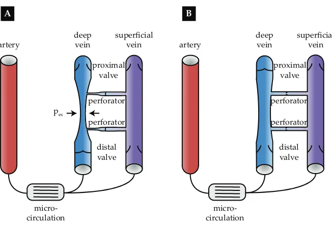
Figure 1: Schematic representation of the muscle pump effect during the A

contrac-tion andBrelaxation phase. During contraction, the deep vein collapses due to the

ex-travascular pressurepex exceeds the intravascular pressure. Venous return is increased,

whereas back-flow and flow to the superficial system is blocked by the distal and per-forator valves. During the relaxation, the deep vein is refilled from both the artery and the superficial vein, while the perforator valves open and the proximal valve is closed to prevent back-flow. Figure was adapted from Keijsers et al. [2015]

1

Introduction

During exercise several complex haemodynamic regulation mechanisms are activated to ensure sufficient supply of oxygen and nutrients, and removal of waste products. In-creased understanding of these individual mechanisms and their interaction is needed to fully characterize the dynamics of blood flow during exercise. At the onset of exercise, the blood flow within muscle in the lower limb increases significantly depending on the arterio-venous pressure drop and the peripheral resistance. These are influenced by both mechanical effects during muscle contraction and relaxation (the muscle pump effect) and the vasodilatory state of the arterioles. However, the exact contribution of these two mechanisms to the blood flow increment at the onset of exercise is still a matter of debate [Tschakovsky and Sheriff, 2004]. Three hypotheses are currently described in literature: the first states that flow augmentation is primarily caused by the muscle pump effect, the second claims that regulation of peripheral resistance is the major determinant. The third hypothesis considers both mechanisms to be important.

As a result of calf muscle activation, the muscle pump effect increases venous return by collapsing the deep veins embedded within the muscle. Furthermore, backflow towards the arterial system and into the superficial venous system is prevented by closure of the distal and perforating venous valves respectively (Figure 1A) [Rowell, 1993]. Arterial inflow rises during subsequent muscle relaxation as the perfusion pressure is increased due to the pressure shielding of the closed proximal valve (Figure 1B) [Rowell, 1993]. Furthermore, the opening of the distal and perforating valves [Meissner, 2005] allows venous refilling from both the arterial and superficial venous system. In summary, the muscle pump effect increases blood flow through an increase in arterio-venous pressure drop.

model. Although the model was able to simulate the increased venous return during muscle contraction and the elevated arterial flow during muscle relaxation, the predicted flow augmentation was low compared to the increase in arterial flow increase measured

duringin vivo calf muscle contractions [N˚adland et al., 2009]. Based on the debate in

literature [N˚adland et al., 2009, Tschakovsky et al., 1996], it was proposed that vasodila-tion could be the missing component in the model. Furthermore, the simulated arterial baseline flow in the tilted position was equal to the baseline flow in the supine posi-tion, which was in strong contrast with the50%decay observedin vivo[N˚adland et al., 2009]. These postural changes can be attributed to changes in peripheral resistance due to myogenic vasoconstriction and a global increase in peripheral resistance [N˚adland et al., 2009]. Therefore, in this study our previous model is extended to include regulation of vascular tone.

Regulation of vascular tone in skeletal muscle tissue is not based on a single mech-anism, but involves the interaction between the local myogenic, local metabolic and global baroreflex regulation [Joyner and Casey, 2015]. Myogenic regulation protects the capillaries against high pressures by vasoconstriction as transmural pressure increases [Boron and Boulpaep, 2003]. The metabolic mechanism induces vasodilation when the amount of metabolites accumulates, thereby regulating the oxygen delivery and removal of waste products [Boron and Boulpaep, 2003, Joyner and Casey, 2015]. Finally, the barore-flex initiates vasoconstriction when central pressure detected by the baroreceptors in the aortic arch and the carotid artery decreases. In addition, the baroreflex affects heart rate, cardiac contractility and venous unstressed volume [Boron and Boulpaep, 2003, Rowell, 1993]. A combined regulation model including all three components is thus required to describe the resulting vascular tone. As all three mechanisms respond to different param-eters and with different time delays, each should be modelled as a separate component. The definition of specific parameters for each mechanism, allows us to examine the rela-tive activation of the three mechanisms during muscle contraction and relaxation. Previous numerical studies of regulation of vascular tone have focussed on cerebral auto-regulation or the baroreflex. Ursino [1988] developed a model for cerebral auto-auto-regulation including a neurogenic and endothelial response in addition to the myogenic and metabolic mechanism. This model was used to investigate the relation between cerebral blood volume and intracranial pressure changes [Ursino and Giammarco, 1991] and applied to examine cerebral regulation under squat exercise and visual stimulation [Spronck et al., 2012]. Models of the baroreflex have been applied to study various physiological re-sponses, e.g. the interaction between the baroreflex and a pulsating heart model [Ursino,

1998], heart rate variability [Ursino and Magosso, 2003], fetal welfare during labor [van der Hout-van der Ja 2013] and heart rate regulation under orthostatic stress [Olufsen et al., 2006]. However,

to our knowledge, no model exists that combines myogenic, metabolic and baroreflex regulation to simulate the vascular tone response to a skeletal muscle contraction. The aim of this study was to determine the importance of the myogenic, metabolic and baroreflex regulation during the different phases of muscle contraction. Therefore, the 1D arterio-venous model as described in Keijsers et al. [2015] was extended with a regulation model for the vascular tone, which includes both the myogenic and metabolic effects de-scribed by Spronck et al. [2012], combined with the baroreflex model of Ursino [1998] to include all three mechanisms. In an initial explorative analysis, the intuitively most important model parameters representing the gain of the myogenic and metabolic

mech-anism were fitted to match the measuredin vivoflow response to a muscle contraction in

model muscle contraction physiological data

sensitivity analysis post-SA analysis circulation model

regulatory model

- 1D pulse wave propagation large vessels - 0D venous valves

- 0D micro-circulation

- myogenic mechanism - metabolic mechanism

- baroreflex

- in supine and tilted position

- collapse deep veins in circulation model

- increase metabolism in regulation model

Figure 4.2B Figure 4.2A

Figure 4.3

Figure 4.8 Figure 4.7

Figure 4.6 Figure 4.5

- assess flow response muscle contraction using ultrasound

- derive supine and tilted fit for validation of the simulations

- Morris screening

- polynomial chaos expansion

- analyse importance parameters - fit supine response

varying G_myo + G_meta - predict response tilted position

- analyse activation regulation

importance regulation mechanisms

importance systemic pressure variation

- fit the either 8 or 4 most important parameters found by SA

- analyse parameter distribution - include pressure

variation in: - pressure BC - baroreflex

Figure 2: Schematic overview of the methods as described in this study including: circu-latory and regulation model, simulation of a muscle contraction, physiological data, and the four analyses performed. For each part the main points are given together with the corresponding figures.

was used. This approach consists of an initial Morris screening and a subsequent general-ized polynomial chaos expansion (gPCE). We conclude with an analysis varying the most important parameters, identified by the sensitivity analysis, to fit thein vivoresponse.

2

Methods

In this section the methods are described and a schematic overview can be observed in Figure 2.

2.1 Model

p₀

p0

p0

poutlet

pinlet

0D inlet BC

0D outlet BC

0D micro-circulation R_a/2

R_a/2

Rv/2

R_v/2 C_v C_a AR1

DV1 DV2

DV3

PV4 PV3 PV2 PV1

VV2 VV1

A

p0

SV1

SV2 SV3

SV4 SV5

VV3 VV4

1D artery 1D deep vein 1D superficial vein 0D venous valve

B

Baroreflex [Ursino1998]

Myogenic [Spronck2012]

Metabolic [Spronck2012]

time delay

Laplace’ law

CO2 production

q p_carotid

T

CO2 level Ameta A_myo

xmeta x_myo xbaro

time delay

time delay

G_meta

G_myo x_tot T r_a Ra

C_a n₂

n3

Figure 3: Model.AModel configuration of the calf circulation including: 1D artery (AR), a 1D deep (DV) and superficial (SV) vein, 0D venous valves (VV), a 0D micro-circulation, a 0D inlet and outlet boundary condition (BC). The length and radius of the 1D elements are not true to scale (geometrical parameters of all 1D segments can be found in Table

1)B Schematic overview of the regulation model including baroreflex, myogenic and

2.1.1 1D Pulse wave propagation: arteries and veins

The hemodynamics in the large arteries and veins is captured using the 1D equations for mass and momentum balance, with blood assumed to be an incompressible Newtonian fluid. The resulting equations read:

C∂ptr

∂t +

∂q

∂z = 0, (1)

∂q

∂t +

∂Av2

z

∂z +

A ρ

∂p

∂z =

2πa

ρ τw+Agz, (2)

whereCis the compliance per unit length,ptr=p−pexis the transmural pressure,pand

pexare the intra- and extravascular pressure respectively,qis the flow,tis the time andzis

the axial coordinate. Furthermore,Ais the cross-sectional area,vzis the velocity in axial

direction averaged over the cross-sectional area,ρis blood fluid density,a=p

A/πis the radius andτw is the wall shear stress. Additionally,gz = ge

g ·ezis the contribution of the gravitational acceleration in the axial direction,gis the magnitude of the gravitational acceleration on earth,e_g is the unit vector in the direction of gravity and e_z is the unit

vector in axial direction.

To obtain an estimation of the wall shear stressτw and the advection term ∂Av

2

z

∂z the

ap-proximate velocity profile is used (see Bessems et al. [2007] for more details). Here, the pressure gradient and the gravitational forces are assumed to be in balance with viscous forces in the boundary layer close to the vessel wall. In the central core inertia forces are assumed to be in balance with the pressure gradient and the gravitational forces. Finally, a constitutive law relating cross-sectional area and pressure, is defined for both arteries and veins.

As the arterial cross-sectional area variations during the cardiac cycle are small under normal conditions, the mechanical characteristics of the arterial wall are modeled with the following linearA, prelation

A=A_ref,A+C(ptr−pref,A), (3)

where A_ref,A is the reference cross-sectional area at reference pressure p_ref,A and C the linearized compliance per unit length at reference pressurep_ref,A. The compliance is de-termined using thin-walled-cylinder theory for a linear isotropic elastic material:

C= ∂A

∂ptr

ptr=pref,A =

2π(1−ν2_)r3

ref,A

hE , (4)

whereν is the Poisson’s ratio,r_ref,A =p

A_ref,A/π is the reference radius,h ≈ r_ref,A/10is the vessel wall-thickness [Westerhof et al., 1969] andEis the Young’s modulus.

Because veins are prone to collapse under low transmural pressures due to e.g. increas-ing extravascular pressure durincreas-ing muscle contraction or gravitational stress, a nonlinear pressure area relationship needs to be considered. Therefore, Shapiro [1977] derived a tube law capturing the venous collapse with anp, A-relation. In order to solve the full system of equations for pressure a fit of the tube law is used as derived in Keijsers et al. [2015].

A=Aref,V

h(p∗

)f+(p∗

) + (1−h(p∗

))f−

(p∗

)

}, (5)

whereAref,Vis the reference cross-sectional area at zero transmural pressure,p∗=ptr/Kp

is the dimensionless pressure andKp is the bending stiffness. The functionsf+andf−

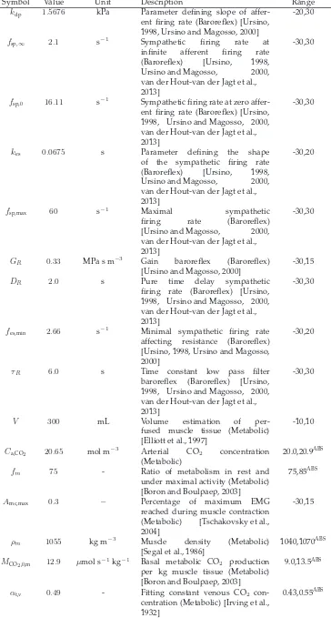
Table 1: Geometrical parameters of the various 1D vessels [M ¨uller and Toro, 2014] as de-picted in Figure 3. The four perforating veins consist of a deep (PV#-D) and a superficial (PV#-S) vein of which the parameters are noted separately.

Vessel Numbering (Figure 3) Radius [mm] Length [cm]

artery AR1 2_.5 34

deep vein DV1 1_.5 2

DV2 1_.5 26

DV3 1_.5 2

superficial vein SV1 3_.5 2

SV2 1_.5 2

SV3 1_.5 26

SV4 1_.5 2

SV5 3_.5 2

perforating vein PV#-S 0_.5 1_.5

PV#-D 0_.5 1_.5

h(p∗

)is a scaling function.

f+(p∗

) = A

+ 0 π

tan−1

p∗

−p+_a p+_b

+π 2 , (6) f−

(p∗

) = B+A

− 0 π

tan−1

p∗

−p−

a p− b + π 2 , (7)

and h(p∗

) = 1

π

tan−1 γp∗ π +π 2 , (8)

whereB, A− 0, p

−

a, p

−

b , A+0, p+a, p+b andγ are fitting constants determining the shape of

theA,p-relation. Venous compliance is calculated as the derivative of cross-sectional area with respect to the transmural pressure.

2.1.2 0D Venous valves

The pressure-flow relation of a venous valve is included using the versatile valve model of Mynard et al. [2012]. As the flow through venous valves is much lower compared to heart valves, the linear viscous forces are included, as in Keijsers et al. [2016].

∆p=Rq+Bq|q|+L∂q

∂t, (9)

where the Poiseuille resistanceR, Bernouilli resistanceBand the inertanceLare defined by

R= 8πηleff

A2

eff

, B = ρ

2A2

eff

and L= ρleff

A_eff, (10)

whereA_effis the effective cross-sectional area,ηis the dynamic blood viscosity, andl_eff=

βl ·rref,V is the effective valve length defined as a multiple βl of the venous reference

radiusr_ref,V=p

A_ref,V/π[Keijsers et al., 2016]. To include valve opening and closing, the effective cross-sectional area is defined to be a function of valve stateζ via the following relation

A_eff= (A_eff,max−A_eff,min)ζ+A_eff,min, (11) where A_eff,min and A_eff,max are the minimal and maximal effective cross-sectional area respectively. Here, maximal effective cross-sectional areaA_eff,max =βA·Aref,Vis defined

as a multipleβA of the reference cross-sectional area Aref,V of the connecting vein. The

ζ = 1). Its value is related via two differential equations for valve opening and closing respectively:

dζ

dt =

(

(1−ζ)Kvo(∆p−dpvalve,0), if∆p > dpvalve,0

ζKvc(∆p−dpvalve,0), if∆p < dpvalve,0

, (12)

where Kvo and Kvc are coefficients determining the opening and closing speed of the

valve. Furthermore,dp_valve,0 is the pressure drop above and below which opening and

closing is initiated.

2.1.3 0D micro-circulation

To account for the pressure drop over the micro-circulation (in the current study defined to include the arterioles, capillaries and venules) and its storage capacity, the micro-circulation model consists of both resistances and compliances. The micro-micro-circulation is split into an arteriolar and venular part, both consisting of two resistancesRi(i=a, v)

in series and a complianceC_i(i=a, v) connected to the extravascular pressure, for which the following relations hold (Figure 3A).

∆p=Riq and

∂ptr

∂t =

1

Ci

q. (13)

Under baseline conditions the total resistance of the two parts is determined by the pres-sure drop over the micro-circulation∆p_bland the time-avaraged baseline flowq_bl accord-ing to

Rtot = ∆pbl

q_bl =Ra+Rv, (14)

whereRvis chosen such that the pressure drop over the venules is400Pa [Boron and Boulpaep,

2003]. Furthermore the baseline total compliance Ctot is derived from a typical

time-constant τ_RC as in a classical single windkessel micro-circulation [Keijsers et al., 2015]. The compliance of the venules is assumed to be much larger than arteriolar compliance [Boron and Boulpaep, 2003]. Therefore, the compliances are distributed as follows

C_a= 0.3·C_tot and C_v= 0.7·C_tot. (15)

The above equations for resistance and compliance relate to the baseline conditions. However, for the arteriolar part of the micro-circulation the resistance and compliance are regulated by vascular tone as described in the following subsection.

2.1.4 Regulation of vascular tone

Regulation of the vascular tone in muscular tissue is based on the following mechanisms (Figure 3B):

• Myogenic regulation: protecting the capillaries against excessive pressures

• Metabolic regulation: matching the blood flow to the oxygen demand

• Baroreflex regulation: aiming to maintain the level of systemic pressure

The regulation model is based on the implementation of cerebral auto-regulation as de-scribed by Spronck et al. [2012]. In this study, each regulation mechanisms is included in-dividually and represented by a regulatory statexi. The myogenic regulatory statexmyo

is derived from the arteriolar wall tensionT and has a time constantτmyo. The metabolic

Spatial pressure m(z) [−]

Z−coordinate [m] A

0 0.1 0.2 0.3 0

0.5 1

Temporal pressure k(t) [−]

Time [s]

B

0 2 4

0 0.5 1

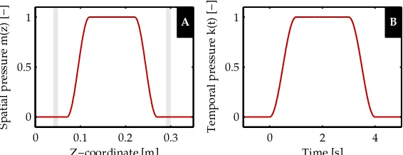
Figure 4: Extravascular pressure of the deep veins is increased to simulate a muscle con-traction. PlotAandBshow the spatialm(z)and temporalk(t) course of extravascular pressure as applied to the deep venous elements respectively (see Appendix A for the full equations ofm(z)andk(t)). The grey areas in the spatial plot indicate the location of the venous valves. [Keijsers et al., 2015]

which is derived from the CO2-production and the blood flow. The latter two regulatory

mechanism are included as described by Spronck et al. [2012], but the metabolic mecha-nism is adjusted to induce metabolic activation upon muscle contraction instead of cere-bral activity, as included by Spronck et al. [2012]. Furthermore, tissue specific parameters are updated to match muscle tissue. Finally, the baroreflex regulatory statexbarois based

on the carotid pressure, which is derived from the pressure at the heart level based on the hydrostatic column. The baroreflex implementation is based on the model based on the study of Ursino [1998]. The total regulatory state is calculated as the weighted sum of the three mechanisms, each having a specific gain:Gmyo,Gmeta andGbaro. The total

regula-tory state is translated to arteriolar wall tension, which is subsequently converted to the arteriolar radius using Laplace’s law. Finally, the arteriolar radius is used to determine the change in peripheral resistance and compliance. For completeness, the equations de-scribing the activation of the three regulation mechanisms and how they affect a change in resistance and compliance are given in Appendix B.

2.1.5 Boundary conditions

Both the inlet of the 1D arterial and the outlet of the 1D venous part are connected to a three element windkessel model representing the proximal vasculature. Each wind-kessel element consists of two resistances in series and a compliance connected to the extravascular pressurep0 (Equation (13)). The total windkessel resistance is the sum of the Poiseuille resistances of the proximal vasculature, based on the geometrical param-eters of the arterial and venous tree published by M ¨uller and Toro [2014]. Similarly, the inlet and outlet compliance is the sum of the compliances of the proximal vasculature based on Equation (4) and the derivative of Equation (5) times the length respectively. At the inlet and outlet the pressure is set to a time-averagedp_inletandp_outletrespectively. When a head up tilt position is simulated the hydrostatic column up to the heart is added to both the inlet and outlet pressure.

The model formulation described above is completed for the current application by defin-ing the form of the muscle contraction.

2.1.6 Simulating muscle contraction

pres-sure. Similar to Keijsers et al. [2015], a muscle contraction is simulated by an increase in extravascular pressure included in the equation for mass balance and the venous consti-tutive law (Equation (1) and (5) respectively). The extravascular pressure is defined by the following relation

pex=pex,max·k(t)·m(z), (16)

wherep_ex,max is the maximal extravascular pressure, and k(t) andm(z) are the tempo-ral and spatial course of extravascular pressure, respectively. The latter can be observed in Figure 4, and the full equations are give in Appendix A. The influence of the mus-cle contraction on the superficial veins is assumed to be negligible due to their location outside the muscle tissue. Furthermore, due to the high arterial pressure the influence of the muscle contraction on the arterial cross-sectional area is also assumed to be neg-ligible. Finally, the mechanical influence on the micro-circulation is also assumed to be negligible due to its viscous character (in Equation (13) and (24)) [Gray et al., 1967]. Al-though contradicted in some studies [Tschakovsky et al., 1996], few experimental studies hypothesize the decrease in transmural pressure could induce myogenic vasodilation [Tschakovsky and Sheriff, 2004], but implementation of this theory requires more accu-rate knowledge of the magnitude of extravascular pressure and is therefore neglected. The increase in metabolism due to a muscle contraction is included in the metabolic mechanism of the regulation of vascular tone via muscle activationAmc(Equation (37)).

Because the flow increase due to a muscle contraction increases linearly with increas-ing contraction intensity [Tschakovsky et al., 2004], muscle activation is defined to follow the contraction pattern defined by the extravascular pressure and reaches a maximum of Amc,maxcorresponding to the percentage of maximum electromyogram (EMG) activity:

A_mc=A_mc,max·k(t). (17)

2.1.7 Numerical implementation

The model equations were implemented in the finite element package SEPRAN (Inge-nieursbureau SEPRA, Leidschendam, the Netherlands) using the computational method described by Kroon et al. [2012]. Time discretization was included based on an implicit

Euler scheme with a time step of ∆t = 1.0 ms and spatial discretization based on the

trapezium rule with element size∆z = 1.0 cm for arterial and superficial venous

seg-ments, and∆z= 0.5cm for the deep venous segments, which is necessary to capture the collapse accurately. The model parameters that are not included in the sensitivity analy-sis are summarized in Table 2. Pre- and post-processing was performed using MATLAB R2012b (MathWorks, Natick, MA, USA).

2.2 Physiological data

Pressure and flow measurements were performed on twelve healthy subjects (29 ±3

years, six male, six female, BMI:23.4±2.3 kg m−2

) during muscle contraction in both the supine and70◦

head up tilt positions. These experiments were approved by the

ethi-cal committee of the Northern Rhine Mediethi-cal Association, Germany (Ethikkommission der

¨

Arztekammer Nordrhein). Subjects were asked to perform a contraction of the left calf

mus-cle corresponding to30%of maximal electromyography (EMG) activity (Ambu Blue

Table 2: Constant model parameters

Symbol Value Unit Description

ρ 1050 kg m−3

Blood mass density [Kenner, 1989]

g 9.81 m s−1

Gravitational acceleration

pref,A 13 kPa Arterial reference pressure [Bessems et al., 2007]

ν 0.5 - Poisson’s ratio [Westerhof et al., 1969]

E 1.6 MPa Arterial Young’s modulus [Westerhof et al., 1969]

Kp 425 Pa Bending stiffness [M ¨uller and Toro, 2014]

A+0 1.37 - Fitting constant [Keijsers et al., 2015]

p+

a -2.53 - Fitting constant [Keijsers et al., 2015]

p+b 3.02 - Fitting constant [Keijsers et al., 2015]

B 0.108 - Fitting constant [Keijsers et al., 2015]

A−

0 1.28 - Fitting constant [Keijsers et al., 2015]

p−

a -1.49 - Fitting constant [Keijsers et al., 2015]

p−

b 2.03 - Fitting constant [Keijsers et al., 2015]

γ 4 - Fitting constant [Keijsers et al., 2015]

η 4.5 mPa s Dynamic blood viscosity [Letcher et al., 1981]

βl 1.0 - Effective valve length ratio [Keijsers et al., 2016]

Aeff,min 1.0 10

−20

m2

Minimal effective valve cross-sectional area [Mynard et al., 2012]

βA 0.65 - Effective valve cross-sectional area ratio

[Keijsers et al., 2016]

Kvo 0.3 Pa

−1

s−1

Valve opening constant [Mynard et al., 2012]

Kvc 0.3 Pa

−1

s−1

Valve closing constant [Mynard et al., 2012]

dpvalve,0 0 Pa Valve opening and closing pressure drop

[Keijsers et al., 2016]

τRC 2.0 s Typical time constant for windkessel element [Keijsers et al., 2016]

pex,max 20 kPa Maximal extravascular pressure [Keijsers et al.,

2016]

frequency of10MHz. The blood flow measurement were performed in pulsed-Doppler

mode. Blood flow was estimated from mean blood flow velocity and vessel diameter using the Poiseuille formulation [Leguy et al., 2009].

To use the experimental data for validation of the simulated muscle flow, the in vivo

flow decay after muscle contraction (10s < t < 50 s) was captured using the following exponential decay relation and a non-linear least squares fit.

qfit(t) =q0+ (qmax−q0)e−(t−tmax)/τ, (18) wheretmax = 10 s,q0 is the baseline flow,qmax is the flow att = tmax andτ is the time

constant of the flow decay. Measurements are excluded from postprocessing when (1)

average arterial pressure is below50mmHg for a whole experiment, (2) femoral artery

flow was only measured successful during part of the experiment or (3) the quality of the flow fit was too low (R2

adj <0.6). An average of the pressure and femoral artery flow was

derived in the supine and head up tilt positions using the following relation

x(t) = 1

Nsubj

Nsubj X

isubj 1

NMC,isubj

NMC,isubj

X

iMC

x_isubj,iMC(t), (19)

whereNsubjis the number of subjects,NMC,isubj is the number of muscle contractions

per-formed by subjecti_subjandxisubj,iMC(t)is the waveform obtained during muscle

contrac-tioni_MCof subjecti_subj. The corresponding intersubject standard deviation was derived using the following relation:

σ2(t) = 1

N_subj−1 Nsubj

X

isubj

xisubj −x(t) 2

Art pres [mmHg]

A MC

A MC

−100 0 10 20 30 40 50

50 100

Time [s]

Fem art flow [m

3 /s] _BB MCMC

−10 0 10 20 30 40 50

0 5 10 15

x 10−6

Supine Tilted Supine fit Tilted fit

Figure 5: Heartbeat average ofAthe finger pressure andBfemoral artery flow response

to a muscle contraction in supine (red) and head up tilt (blue) position. The gray area indicates the 4-s muscle contraction (MC). Furthermore, the fit (−−) to the flow response is included, where its uncertainty is indicated with the shaded area around (light gray indicates the overlap). The dotted line (··;0 < t < 10s) indicates the uncertain part of the flow curve due to measurement difficulties. Fitting parameters and their standard deviation can be found in Table 3.

Table 3: Fitting parameters of the flow decay after muscle contraction using the following equation:q_fit(t) =q0+ (qmax−q0)e−(t−tmax)/τ

q0[mL/s] qmax[mL/s] τ[s] Supine 2_.8±1_.5 12_.1±5_.6 8_.4±1_.6

Head up tilt 1_.2±1_.1 9_.2±5_.0 6_.4±2_.2

wherexisubj(t)is the mean response of subjectisubj. The resulting time averaged pressure

and femoral artery flow are shown in Figure 5A and B respectively, with the supine mea-surement in red and the head up tilt in blue. The area around the fitted curve represents one standard deviation from the average fit.

2.3 Simulations and analysis

The first aim is to match the simulated flow response during a supine muscle contrac-tion to the fit of the measured data (Figure 5B), to gain insight into the importance of the various regulation mechanisms. An explorative local analysis including variation ofxinit,

Tmax,0,GmetaandGmyo, identifiedGmeta andGmyoas the major determinants. Therefore,

G_meta andG_myowere varied (−25 < G_meta < −15; dG_meta = 1and0.5 < G_myo < 1.5; dGmyo = 0.25) during the fitting procedure, while keeping all other regulation

param-eters at their baseline values (55 model evaluations). The best three sets of gains are derived based on the least square of the difference between the simulated flow response and thein vivofit.

ǫ=

Z 50s

t=10s

p

(qsim−qfit)2dt. (21)

Time [s]

B A

Sx1 S_x1,x2

Sx1,x3 S_x3 Sx1,x2,x3

MC Arterial flow

50 in vivo fit

q_hut,bl

ε

sup

ε

hut

simulation

10 0 q_sup,10 q_hut,10

30

supine

tilted

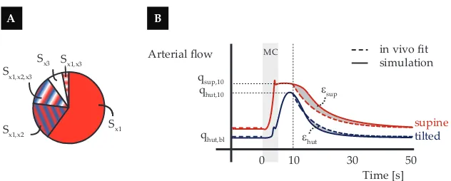
Figure 6: Sensitivity analysisASchematic visualisation of the distribution of the output

variance over the various input parameter and their interactions. Si =main sensitivity

index,Sij =second order effect,Sijk=third order effect.BOutput of interest visualized

in a plot of the flow response to a muscle contraction in supine and tilted position.

In the above mentioned analysis a constant pressure is used as an input for the baroreflex

and the inlet boundary condition. However,in vivothe systemic pressure shows a small

increase during and a decrease after muscle contraction (Figure 5). In a second analysis the influence of this pressure fluctuation via the systemic pressure and the baroreflex reg-ulation on the flow response was investigated. For this the best parameter set, derived in the first analysis, was used to repeat the supine and tilted simulations with the following adaptations: (1)in vivo pressure is used as an input for the baroreflex andp_inlet remains

unchanged compared to the previous simulations; (2)in vivopressure is used as an input

for the baroreflex as well as forpinlet.

2.4 Sensitivity analysis

To investigate the importance of all regulation parameters on the flow response to a mus-cle contraction and to validate the choice to derive the fit based on onlyGmeta andGmyo

as described in the previous section, a global sensitivity analysis was performed. Si-multaneous variation of the input parameters within their uncertainty range enables the derivation of the variance in the simulated flow response. Each fraction of this output variance can be allocated to individual parameters or interaction between two or more input parameters (Figure 6A). The influence of an individual input parameter is captured by the main sensitivity indexSi, which can be interpreted as the expected reduction in

output variance if the true value would have been known. The contribution of interac-tion between two or more parameters is captured by the higher order effects (Sij, Sijk, ...)

[Eck et al., 2016].

2.4.1 Output of interest

The following parameters, describing the flow response to a muscle contraction in both supine and tilted position, are used as outputs of interest:

• qsup,max: Flow in supine position10safter the onset of muscle contraction.

• ǫsup =R_t50₌₁₀s_s q

(qsim,sup−qfit,sup)2: Root mean square of the difference between the

simulation and the fit of the flow response to a muscle contraction in the supine position.

• q_hut,bl: Baseline flow in the tilted position.

• ǫ_hut =R50s

t=10s

p

(q_sim,hut−q_fit,hut)2_{: Root mean square of the difference between the} simulation and the fit of the flow response to a muscle contraction in the tilted position.

2.4.2 Input parameters

The sensitivity analysis was performed while varying all input parameters of the regula-tion model. A descripregula-tion of these parameters can be found in Table 4, along with their baseline value and the range used for the sensitivity analysis. The uncertainty ranges are based on literature values or values resulting in a physiological flow response determined by a local sensitivity analysis (results not shown). From this local sensitivity analysis, it was concluded thatrm(the radius at which maximal tension can be reached) andrt(the

constant defining the shape of the maximal tension curve) should be fixed, as even small variation resulted in non-physiological responses or decreased model stability.

Table 4: Model input parameters included in the sensitivity analysis. Uncertainty range is given in percentages, unless indicated with superscript ABS when the absolute range is given. The uncertainty range is based on literature values and is adapted when the local sensitivity analysis indicated unphysiological outputs or decreasing in model stability.

Symbol Value Unit Description Range

σe,0 1.49 kPa Parameter for elastic tension model (Laplace) [Ursino and Giammarco, 1991]

-10,7.5

Kσ 4.5 - Parameter in tension model

(Laplace) [Ursino and Giammarco, 1991]

-10,10

ra,0 75.0 µm Arteriolar radius in

un-stressed condition (Laplace) [Ursino and Giammarco, 1991]

-10,10

σc 5.51 kPa Stress contribution of

col-lagen fibers (Laplace)

[Ursino and Giammarco, 1991]

-10,10

rha,0 0.33 - Unstressed arteriolar wall

thick-ness relative to radius (Laplace) [Nordborg et al., 1985]

-10,10

ηa 6.37 kPa s Arteriolar wall viscosity (Laplace) [Ursino and Giammarco, 1991]

-10,10

nm 1.75 - Parameter for smooth

mus-cle tension model (Laplace) [Ursino and Giammarco, 1991, Ursino and Lodi, 1998]

-10,7.5

Tmax,0 5.0 Pa Smooth muscle tension in

basal condition (Laplace) [Ursino and Giammarco, 1991, Ursino and Lodi, 1998]

4.0,5.5ABS

xinit −0.5 - Offset regulation state (Laplace) -0.6,-0.45ABS

pn 13.3 kPa Reference pressure

barore-flex model (Baroreflex)

[Boron and Boulpaep, 2003]

-10,10

fab,min 2.52 s

−1

Minimal afferent firing rate (Baroreflex) [Ursino, 1998, Ursino and Magosso, 2000, van der Hout-van der Jagt et al., 2013]

-30,30

fab,max 47.78 s

−1

Maximal afferent firing rate (Baroreflex) [Ursino, 1998, Ursino and Magosso, 2000, van der Hout-van der Jagt et al., 2013]

Table 4 – continued from previous page

Symbol Value Unit Description Range

kdp 1.5676 kPa Parameter defining slope of affer-ent firing rate (Baroreflex) [Ursino, 1998, Ursino and Magosso, 2000]

-20,30

fsp,∞ 2.1 s −1

Sympathetic firing rate at infinite afferent firing rate (Baroreflex) [Ursino, 1998, Ursino and Magosso, 2000, van der Hout-van der Jagt et al., 2013]

-30,30

fsp,0 16.11 s

−1

Sympathetic firing rate at zero affer-ent firing rate (Baroreflex) [Ursino, 1998, Ursino and Magosso, 2000, van der Hout-van der Jagt et al., 2013]

-30,30

kes 0.0675 s Parameter defining the shape

of the sympathetic firing rate (Baroreflex) [Ursino, 1998, Ursino and Magosso, 2000, van der Hout-van der Jagt et al., 2013]

-30,20

fsp,max 60 s−1 Maximal sympathetic

firing rate (Baroreflex)

[Ursino and Magosso, 2000, van der Hout-van der Jagt et al., 2013]

-30,30

GR 0.33 MPa s m

−3

Gain baroreflex (Baroreflex) [Ursino and Magosso, 2000]

-30,15

DR 2.0 s Pure time delay sympathetic

firing rate (Baroreflex) [Ursino, 1998, Ursino and Magosso, 2000, van der Hout-van der Jagt et al., 2013]

-30,30

fes,min 2.66 s

−1

Minimal sympathetic firing rate affecting resistance (Baroreflex) [Ursino, 1998, Ursino and Magosso, 2000]

-30,20

τR 6.0 s Time constant low pass filter

baroreflex (Baroreflex) [Ursino, 1998, Ursino and Magosso, 2000, van der Hout-van der Jagt et al., 2013]

-30,30

V 300 _{mL Volume estimation of}

per-fused muscle tissue (Metabolic) [Elliott et al., 1997]

-10,10

Ca,CO2 20.65 mol m −3

Arterial CO2 concentration

(Metabolic)

20.0,20.9ABS

fm 75 - Ratio of metabolism in rest and

under maximal activity (Metabolic) [Boron and Boulpaep, 2003]

75,85ABS

Amc,max 0.3 − Percentage of maximum EMG

reached during muscle contraction (Metabolic) [Tschakovsky et al., 2004]

-30,15

ρm 1055 kg m

−3

Muscle density (Metabolic) [Segal et al., 1986]

1040,1070ABS

MCO₂,0,m 12.9 µmol s

−1

kg−1

Basal metabolic CO2 production

per kg muscle tissue (Metabolic) [Boron and Boulpaep, 2003]

9.0,13.5ABS

αt,v 0.49 - Fitting constant venous CO2

con-centration (Metabolic) [Irving et al., 1932]

Table 4 – continued from previous page

Symbol Value Unit Description Range

βt,v 11.5 mol m

−3

Fitting constant venous CO2

con-centration (Metabolic) [Irving et al., 1932]

9.7,13.3ABS

Cv,CO2,0 22.34 mol m −3

Venous CO2 concentration at rest

(Metabolic) [Geers and Gros, 2000]

22.1,23.0ABS

Gmeta −15 - Gain for metabolic mechanism

(Metabolic)

-25,-10ABS

τmeta 15.0 s Time-constant metabolic regulation (Metabolic) [Ursino and Lodi, 1998]

12,18ABS

Gmyo 0.75 - Gain for myogenic mechanism

(Myogenic)

0.1,5ABS

τmeta 7.0 s Time-constant myogenic regulation

(Myogenic) [Ursino and Lodi, 1998]

4,9ABS

2.4.3 Morris screening and general polynomial chaos expansion

To derive the output variance and the sensitivity indices in a computationally efficient manner, the two-step approach described by Donders et al. [2015] was used. In the first step non-important model parameters are identified by using a Morris screening. In the second step the generalized polynomial chaos expansion method is applied to the re-duced input space, resulting in a metamodel from which the sensitivity indices can be calculated straightforwardly [Huberts et al., 2014]. The metamodel consists of orthogonal polynomials dependent on the model parameters and with output-specific coefficients,

which are derived by a least-square regression of the metamodel andNsimulations. The

accuracy of the metamodel is determined by the quality of the regression, for which a sufficient number of model evaluations is needed. In the current study a metamodel con-taining orthogonal polynomials up to the third order is derived based on 13485 model evaluations (CP U ≈63h, using 25 cores). The number of model evaluations is based on: N = z+_zk

·q, wherez = 3is the order of the metamodel,k= 28is the number of input parameters of the reduced input space andqis set to 3 to have sufficient simulations to obtain a good regression.

2.4.4 Post sensitivity analysis

To investigate how well the important parameters identified in the sensitivity analysis

can fit thein vivo response two additional sets of simulations were performed. First,

all parameters withST > 0.05for at least one output of interest were varied randomly

overk∗ 500 simulations, withk the number of parameters. Second, the same process

was carried out for all parameters withST > 0.10. For both sets of simulations it was

investigated which simulations were in good agreement with thein vivofit, i.e. within the standard deviation of thein vivofit. A second subset is defined to include all simulation within half the standard deviation. Finally, it is analysed how the input parameters of these subsets of simulations were distributed over the input space.

3

Results

This section first reports how the activation of the regulation mechanisms influences the

agreement between the flow response and the in vivodata. Secondly, the influence of

Regulation state [−]

Supine position

A

vaso−constriction

vaso−dilation MC

−10 0 4 10 20 30 40 50 −3

−2 −1 0 1 2 3

Arterial flow [mL/s]

Time [s]

C _MC

−100 0 4 10 20 30 40 50 1

2 3 4 5

Tilted position

B _MC

−10 0 4 10 20 30 40 50 −3

−2 −1 0 1 2 3

Time [s]

D _MC

−100 0 4 10 20 30 40 50 1

2 3 4 5

x_baro x

meta x

myo x

tot

In vivo Simulations

Figure 7: Regulatory response to muscle contraction in supine and tilted position, de-picted in the left and right column respectively. In plotAandBthe regulation state of

the various mechanisms is shown over time: baroreflex (−−), metabolic (−·), myogenic

(··) regulation and the sum of the three (−). Here, the negative state corresponds to va-sodilation and the positive state to vasoconstriction. The resulting arterial flow is shown in plotCandDtogether with the fit to the in vivoresponse (−·). The three simulations

best matching thein vivoresponse are depicted in color. The remaining simulations (as

described in Section 2.3) are visualized together in the gray area. To show the general patterns some individual responses are depicted in dark gray.

3.1 Baseline simulations

The regulatory response to a muscle contraction in the supine position was simulated while varying the gain of the myogenic and metabolic mechanism. The variation in reg-ulatory responses and arterial flow are indicated by the gray region either side of the curve in Figure 7A and C respectively. The period of muscle contraction (MC) is indi-cated by the shaded region (0 < t < 4s). The arterial flow responses which best match

thein vivomeasurement (−·plus the standard deviation indicated by the blue area) are

visualised in color. These parameters values are used to repeat the simulation in the tilted position, for which the results are shown in Figure 7B and D. For the best flow results the regulatory state of the baroreflex (−−), metabolic (−·) and myogenic (··) mechanism are also shown in color.

the muscle contraction and a gradual decay starting att ≈ 10s, which closely matches

thein vivoresponse (Figure 7C). Most of the remaining flow responses show waveforms

that are parallel to each other, although some simulations cross due to a difference in decay (Figure 7C).

In the tilted position, the baroreflex and to a lesser extent the myogenic mechanisms induce a vasoconstriction at baseline (−10 < t <0s). After muscle contraction (t >4s), the metabolic response induces a vasodilation, slightly inhibited by the vasoconstrictive response of the myogenic mechanism and baroreflex (Figure 7B). Finally, arterial flow

increases after muscle contraction and decreases back to baseline, matching thein vivo

response (Figure 7D).

3.2 Influence of systemic pressure

The influence of the fluctuation in systemic pressure on the flow response to a muscle contraction is investigated. For this, the best fit found in the previous section is compared to a simulation with the pressure fluctuations included only in terms of the baroreflex regulation and a simulation with the pressure fluctuation applied at the inlet as well as the baroreflex. The regulatory (top) and flow (bottom) response to a muscle contraction in the supine (left) and tilted (right) position are shown in Figure 8.

In the supine position the three simulations all start at the same baseline and show a similar decay fort >10s(Figure 8C). Peak flow (5< t <10s) is lower once the pressure fluctuation is applied via baroreflex regulation (green line). In the case where the pressure fluctuation is also applied as an inlet boundary condition (orange line) a fast decrease is observed shortly after muscle contraction followed by a plateau. In the tilted position all three simulations start at the same baseline (Figure 8D). The flow decay fort >10 s is faster for both simulations with thein vivopressure applied compared to the original

simulation, but remain close to the fit of the in vivo response (dashed dark blue line).

Furthermore, peak flow is higher and is reached sooner following muscle contraction if

thein vivopressure is used.

3.3 Sensitivity analysis

3.3.1 Morris screening

From the Morris screening the following parameters were found to be unimportant:

pa-rameter for smooth muscle tension model nm, minimal afferent firing rate (baroreflex)

f_ab,min, parameter defining shape of sympathetic firing rate (baroreflex)kes, pure time

de-lay of sympathetic firing rate (baroreflex)D_R, percentage of maximum EMGA_muscle,max

and basal metabolic CO2-productionMCO2,0,m. Excluding these six parameters from the

polynomial chaos expansion reduces the required number of simulations from 23310 to 13485.

3.3.2 Polynomial chaos expansion

The quality of the derived metamodels, captured by the descriptive error, is shown in Table 5. This gives the part of the variance that could not be captured by the metamodel. For theǫsupandǫhutthe descriptive error is relatively large; 0.14 and 0.10 respectively.

The total sensitivity indices for all outputs of interest are shown in Table 6. The input

parameters are arranged in order of importance and only contributions greater than1%

are shown. The myogenic gainGmyo is the most important parameter for all outputs of

Regulation state [−]

Supine position

A

vaso−constriction

vaso−dilation MC

−10 0 4 10 20 30 40 50 −3

−2 −1 0 1 2 3

Arterial flow [mL/s]

Time [s]

C _MC

−100 0 4 10 20 30 40 50 1

2 3 4 5

Tilted position

B _MC

−10 0 4 10 20 30 40 50 −3

−2 −1 0 1 2 3

Time [s]

D _MC

−100 0 4 10 20 30 40 50 1

2 3 4 5

x baro x_meta x

myo x_tot

In vivo fit Original In vivo p_baro In vivo p

baro and p

inlet

Figure 8: Influence of variation in systemic pressure on the regulatory response to mus-cle contraction in supine and tilted position (left and right column respectively). In plot

AandBthe regulation state of the various mechanisms is shown over time: baroreflex

(−−), metabolic (··), myogenic (−·) regulation and the sum of the three (−). Here, the negative state corresponds to vasodilation and the positive state to vasoconstriction. The resulting arterial flow is shown in plotCandDtogether with the fit to thein vivoresponse (−·). The various colors represent the original simulation (red line),in vivo pressure ap-plied at the baroreflex (green line) andin vivopressure applied to both the baroreflex and the inlet boundary condition (orange line).

Table 5: Quality of the metamodel for each output of interest:qmax,sup,ǫsup,qbl,hut,qmax,hut

andǫ_hut. The error measure1−R2can be interpreted as the residual variance that could not be captured by the metamodel.

qmax,sup ǫsup qbl,hut qmax,hut ǫhut

Table 6: Total sensitivity indices of all the outputs of interest:qmax,sup,ǫsup,qbl,hut,qmax,hut

andǫ_hut. The input parameters are arranged in order of importance and only

contribu-tions starting at1%are shown.

qmax,sup ǫsup qbl,hut qmax,hut ǫhut

Gmyo 0.79 0.72 0.55 0.64 0.47

Gmeta 0.08 0.17 0.18 0.30

xinit 0.02 0.38 0.04 0.11

τmeta 0.16 0.02 0.09

Cv,CO₂,0 0.02 0.06 0.05 0.09

Ca,CO2 0.02 0.06 0.05 0.09

r0 0.06 0.06 0.02 0.01 0.02

Tmax,0 0.03 0.03 0.01 0.03 0.05

τmyo 0.08 0.03

fab,max 0.01 0.02 0.02 0.05

fm 0.02 0.05 0.01 0.02

GR 0.02 0.02 0.02 0.04

pn 0.01 0.02 0.04 0.01 0.02

kdp 0.01 0.01 0.02 0.03

Kσ 0.03 0.03

fes,min 0.02 0.01 0.03

fsp,∞ 0.01 0.01 0.03

fsp,0 0.02 0.01

σe0 0.02

rh0 0.02

V 0.02

αtv 0.02

σc 0.01

ηa 0.01

fsp,max 0.01

τR 0.01

ρm 0.01

βtv 0.01

metabolic time constantτmetaall contribute more than10%to the variance for at least one

output of interest. This is in line with the first local analysis where a fit was derived based onGmyo andGmeta. Four other parameters have a contribution larger than5%: Cv,CO2,0,

Ca,CO2, r0 andτmyo. All other parameters have a smaller contribution, but they do all

contribute to the variance of the output.

The main sensitivity indices and higher order interactions are shown in Figure 9, where the main sensitivity indicesSiare shown as ellipsoids, the second order interactions are

indicated by an arrow and the third order interactions by a shaded area. The myogenic gain contributes most to the output variance; it has the highest main sensitivity index for all outputs of interest and is present in all of the main interactions. Furthermore, the metabolic gainGmeta, the initial regulation statexinitand the metabolic time constantτmeta

all have a main sensitivity index and/or interaction larger than 0.05 for at least one output of interest. The sums of the sensitivity indices (bottom of each subfigure) show that most of the variance is captured by individual contributions (Si). However, forǫsup andǫhut

a significant contribution to the variance comes from interactions between parameters. The contribution of the parameters varies for each regulation mechanism. The influence

of the metabolic parameters is mainly observed in the maximum flow and ǫ outputs.

Σ _S

i = 0.87 Σ Sij = 0.06 Σ Sijk = 0.07

E q_max,hut

C_a,CO2 Si= 0.03 C_v,CO2,0 Si= 0.03 Tmax,0 Si= 0.02 xinit Si= 0.01 Gmyo Si= 0.58 Gmeta Si= 0.14

Σ _S

i = 0.87 Σ Sij = 0.09 Σ Sijk = 0.04 Sij= 0.03 Sij= 0.01

K_s r₀

B q_max,sup

C a,CO2 Si= 0.02

C v,CO2,0 Si= 0.02

T_max,0 Si= 0.02 f_m

Si= 0.02 G_myo Si= 0.71

Gmeta Si= 0.07 C v,CO2,0 Si= 0.03 C a,CO2 Si= 0.02

Σ _S

i = 0.59 Σ Sij = 0.26 Σ Sijk = 0.15

F ε

hut

T_max,0 Si= 0.02

f_ab,max Si= 0.01

G_R Si= 0.01 x_init

Si= 0.04

Sij= 0.02 Sij= 0.02

Sijk= 0.01 Sijk= 0.01

τ meta Si= 0.06

S_ij= 0.09

G_meta Si= 0.13

G_myo Si= 0.23 Σ _S

i = 0.92 Σ Sij = 0.07 Σ Sijk = 0.01

D qbl,hut

r₀ Si= 0.02 p_n

Si= 0.04

G_R f_ab,max Sij= 0.01 Sij= 0.01 Sij= 0.01 G_myo Si= 0.48

x_init Si= 0.36

G_meta C

v,CO2,0

C_a,CO2 f_m

Σ _S

i = 0.46 Σ Sij = 0.38 Σ Sijk = 0.16

C ε

sup

r₀ Si= 0.02 τ

myo Si= 0.04

τ meta Si= 0.04

Sij= 0.02

Sij= 0.03 Sij= 0.03

Sij= 0.04 Sij= 0.01

S_ij= 0.12

S_ij= 0.08

Gmyo Si= 0.34 x_i

Si = ...

Second order interaction Sij = ... if Sij > 0.05 xj

x_i Sij= ...

xi

x_k xj Sijk= ...

Third order interaction Main sensitivity index if S_i > 0.05

A Legend

Figure 9: Results of the sensitivity analysis for all the outputs of interest: Bqmax,sup,C

rmsqsup,Dqbl,hut,Eqmax,hutandFrmsqhut. The main sensitivity index is visualised in a

circle, the second order interaction with an arrow and the third order interaction with an

area. For clarity only the contributions larger than1%are shown. The most important

parameters and interactions (with a contribution more than 5%) are highlighted with

Flow supine [mL/s]

Variation parameters S T > 0.05

A

−100 0 10 20 30 40 50

2 4 6

Flow tilted [mL/s]

Time [s] C

−100 0 10 20 30 40 50

2 4 6

G_myo G_meta

x_init

τ_meta

C_v,CO 2,0 C_a,CO

2

τ_myo

r₀

Scaled input [−]

E

0 0.5 1

Variation parameters S T > 0.10

B

−100 0 10 20 30 40 50

2 4 6

Time [s] D

−100 0 10 20 30 40 50

2 4 6

All sims Good sims (std) Good sims (std/2) Best sims In vivo

G_myo G_meta

x_init

τ_meta

F

0 0.5 1

Figure 10: Post sensitivity analysis. The flow response of additional simulations varying the input parameters with ST > 0.05 (left column) and ST > 0.10 (right column) in

both supine (AB) and tilted position (CD). For both sets the good simulations (present within one standard deviation and half the standard deviation) are presented in dark gray and the best 10 simulations in color. In the bottom plots (EF) the distribution of the corresponding input parameter is shown.

3.3.3 Post sensitivity analysis

The important parameters identified though the sensitivity analysis were used to perform two sets of simulations: (1) varying all parameters withST >0.05(k= 8) and (2) varying

all parameters withST > 0.10 (k = 4). The flow response in both the supine and tilted

positions together with the distribution of the input parameters is shown in Figure 10. Both sets of simulations are divided into four subsets: (1) the simulations that converged (light gray) (2) the simulations that had a flow response within the standard deviation of thein vivofit (middle gray) (3) the simulation that had a flow response within half a standard deviation (dark gray) and (4) the 10 simulations which best matched the mean

in vivoresponse (colors).

For the first set of 4000 simulations (ST >0.05) 1610 of the 3880 (41%) converged

simu-lations had a flow response within one standard deviation of thein vivo response (mid

light gray area covers the whole input space. However, some combinations never occur;

e.g.GmyoandGmetanever have their maximum value simultaneously. When considering

the simulations within half a standard deviation, a decrease in the input range ofGmyois

observed (Figure 10E). The ten best simulations closely match the meanin vivoresponse

in both positions (Figure 10AC). The distribution of the input parameters is more spread over the input domain once the importance of the parameter decreases (parameter

im-portance decreases from left to right). Whereas the most important parameterGmyohas

relative values between 0.10 and 0.27, values of the less important parameters,Cv,CO2,0,

Ca,CO2,0andτmyo, cover the full input domain.

In the second set of 2000 simulations (ST >0.10) 1104 out of 1961 (56%) converged

simu-lations showed a flow response within thein vivouncertainty (mid gray in Figure 10BD). Considering only half a standard deviation results in only 277 (14%) simulations. Similar to the larger set of simulations, the input parameters of the good simulations (within one standard deviation) had values within their whole uncertainty range (mid gray Figure 10F). Again, not all combinations were present, especially at the lower and upper lim-its of the domains. For the subset within half a standard deviation a decrease in input range ofG_myois observed as for the first set of simulations. Although the value of ǫ_sup andǫhutslightly increased (same order of magnitude), the 10 best simulations still closely

matched thein vivofit. However, now the values ofGmeta show a stronger correlation

with the values ofG_myo, which is in line with the high values found in the sensitivity analysis for the interaction betweenGmyoandGmeta. Furthermore, the range ofGmetahas

shifted to the upper part of the domain, which indicatesGmeta could be fixed within this

range to obtain a good fit.

4

Discussion

The flow augmentation observed at the onset of exercise is hypothesized to be a result of the muscle pump effect, the regulation of vascular tone or a combination of both. In a previous study [Keijsers et al., 2015], we showed that the muscle pump effect alone cannot induce the flow increase observedin vivo. Therefore, in the current study the im-portance of the major mechanisms regulating blood flow during the different phases of a muscle contraction has been investigated in both the supine and tilted position. To inves-tigate these effects our arterio-venous 1D pulse wave propagation model [Keijsers et al., 2015] has been extended with a regulation model accounting for baroreflex, metabolic and myogenic regulation. Model parameters were either taken from literature or deter-mined by fitting the simulated arterial flow response to the measuredin vivoresponse to a muscle contraction in the supine position. The model was then validated by comparing

simulated results with thein vivo measurements in the tilted position without changing

the parameter values obtained from the fit in the supine position. Furthermore, a sensi-tivity analysis has been performed to quantify the importance of the input parameters in the regulation model.

The model was able to capture thein vivo response in the supine position when only

optimizing the values of the myogenic and metabolic gain (Figure 7C). When the same parameters were used to simulate a muscle contraction in the tilted position, again good agreement was found (Figure 7D). The model response replicates two of the main fea-tures of flow variation. Firstly, it matches the flow decay back to baseline after the va-sodilation is initiated following muscle contraction. Secondly, the model captures the decreased baseline flow in the tilted position observedin vivo. Examining the activation of the various regulation mechanisms, the metabolic mechanism is the main vasodilator after muscle contraction in both the supine and tilted position, which is in line within vivo

simu-lations support the hypothesis of N˚adland et al. [2009] that the decrease in baseline flow in the tilted position is a result of the global baroreflex and local myogenic activation. The latter is a result of the decreased carotid pressure and increased arteriolar pressure respectively.

The influence of the variation in systemic pressure via the baroreflex mechanism and the boundary conditions of the model is assessed and is most clearly observed within the first10safter the onset of muscle contraction (Figure 8). The lack of reliablein vivodata shortly after muscle contraction, does not allow any conclusions to be drawn on which implementation is closest to physiology. The relatively small effect during the remaining part of the response (t > 10s) can be explained by the fact that most of the variation in systemic pressure is present shortly after muscle contraction. In thein vivostudy of N˚adland et al. [2009] it was stated that the systemic pressure reduction was too small to have an effect on femoral artery flow. However, based on the combination of the current

model results andin vivomeasurements this statement can neither be confirmed nor

re-jected. Because the current study focusses on the flow decay after muscle contraction and the baseline flow, which are both hardly affected, the systemic pressure variation is not expected to have a large influence on the results.

Based on the sensitivity analysis, the spread in myogenic gainGmyois clearly the most

im-portant parameter (both individually and through interactions) of the regulation model for variance in the simulated flow response to muscle contraction (Figure 9). The uncer-tainty in metabolic gainGmetaalso has a significant contribution to the output variance.

The importance of both gains was expected, because they determine the magnitude of vasodilation. Furthermore, it confirms the choice to varyGmyoandGmetain the first

anal-ysis. The fact thatGmyo is more important than Gmeta may be a result of the sigmoid

function (Equation (30)) that is applied to the total regulation state. Even a small myo-genic activation (i.e. vasoconstriction) will shift the total regulation towards the more sensitive part of the regulation curve. A third important parameter isxinit, which is the

offset of the regulation state. A change inxinitcan shift the regulatory response to a less or

more sensitive region of the regulation curve. This explains the large importance ofxinit

forqbl,hut. The fourth important parameter is the metabolic time-constantτmeta, which is

expectedly important for both ǫoutputs. The fact that the metabolic parameters

dom-inate theǫ output is logical, because the metabolic activation was concluded to be the

main vasodilator after muscle contraction. The baroreflex is almost inactive in the supine position, which is confirmed by the fact that the baroreflex parameters are not present for the supine outputs. Whilst the current model may seem complex, the large contribution of the higher order terms (Sij andSijkin Figure 9) indicates the need of all parameter

in-teractions in capturing the complex physiology of the system and thereby that the model is not too complex.

In the post sensitivity analysis it was concluded that even when only varying the 4 most important parameters (each contributing more than10%), it was still possible to find sim-ulations that strongly resemble thein vivoresponse. The small range found forGmyofor

the 10 best fits confirms the importance ofGmyo. Furthermore, the interaction between

GmyoandGmetawas also confirmed, because high values of the two parameters never

oc-cur simultaneously. Examining the relation betweenGmyo andGmetafor the 10 best fits,

even suggests defining a relation between the two. The large spread of input parameters observed for the subset of simulations within the measurement uncertainty, could indi-cate that the whole input space is not covered. However, analysing the simulations with a flow response within half a standard deviation indicates that if one could reduce the

measurement uncertainty, the input space of the most important parameterGmyocould

be decreased.

ar-teriolar radius as a measure for the regulatory state, because the explicit representation of individual arterioles was not of interest in the current study. Metabolic regulation was included based on a single metabolite, whereas many metabolites are known to act as vasodilator and no single metabolite has been shown to account for the full vasodila-tory response [Joyner and Casey, 2015]. However, the current implementation is in good

agreement with thein vivoresponse, which indicates that the tissue CO2-concentration

is a good surrogate for the general metabolic response. For a correct myogenic activa-tion an accurate pressure level is necessary. As only the calf circulaactiva-tion is included in the 1D part, the hydrostatic column applied to the pressure boundary condition might be overestimated, especially on the venous side. This could be overcome if the proximal vasculature would also be included in the 1D part of the model. However, as the current

model is able to accurately match thein vivo response, it is concluded that the current

model contains sufficient detail to capture the flow response after muscle contraction.

For validation of the developed model,in vivoultrasound measurements were performed

capturing the flow response to a calf muscle contraction in both the supine and tilted po-sitions (Figure 5B). Measured baseline flow in the supine position was observed to be 2.3 times higher than in the70◦

head up tilt position (Table 3), which is in line with the flow decrease observed by N˚adland et al. [2009] in the30◦

head up tilt position. Flow

changes observed following muscle contraction reach peak flow within10sfollowed by

a decay back to baseline within a further minute. This is in accordance with the changes observed by Tschakovsky et al. [1996] following a single forearm contraction and those observed by Wesche [1986] following quadriceps contraction. Although the general flow response is in accordance with previousin vivo studies, the first10 safter the onset of muscle contraction are excluded from the validation, because this part of the measure-ment is less accurate due to measuremeasure-ment difficulties during and shortly after muscle contraction. Improved measurements are necessary for validation of the simulated flow

response in the first10 safter muscle contraction, which could possible be obtained by

fixing the ultrasound probe to the subject.

The quality of the metamodel, captured in the coefficient of determination (1−R2_{), was}

observed to be lower for the outputsǫsup andǫhut. Because both outputs cover a time

range of40s, they include more information, which is more likely to be hard to capture in a metamodel. Furthermore, these effects could be due to the fact that the importance of the parameters excluded by the Morris screening was underestimated. However, the post sensitivity analysis shows that even when varying only the four most important param-eters the model is capable to capture the flow response to a muscle contraction. Another more likely reason is that the variance that could not be captured by the metamodel is a result of the high frequency vibrations present in some simulations, because theǫ out-puts are affected most by these instabilities. Further research is needed to improve model stability. However, the values of the coefficient of determination are still acceptable and are not expected to influence the results.