This is a repository copy of Uncertainty of wheat water use: Simulated patterns and sensitivity to temperature and CO₂.
White Rose Research Online URL for this paper: http://eprints.whiterose.ac.uk/106088/
Version: Accepted Version
Article:
Cammarano, D, Rötter, RP, Asseng, S et al. (46 more authors) (2016) Uncertainty of wheat water use: Simulated patterns and sensitivity to temperature and CO . Field Crops ₂
Research, 198. pp. 80-92. ISSN 0378-4290 https://doi.org/10.1016/j.fcr.2016.08.015
© 2016 Elsevier B.V. This manuscript version is made available under the CC-BY-NC-ND 4.0 license http://creativecommons.org/licenses/by-nc-nd/4.0/
[email protected] https://eprints.whiterose.ac.uk/ Reuse
Unless indicated otherwise, fulltext items are protected by copyright with all rights reserved. The copyright exception in section 29 of the Copyright, Designs and Patents Act 1988 allows the making of a single copy solely for the purpose of non-commercial research or private study within the limits of fair dealing. The publisher or other rights-holder may allow further reproduction and re-use of this version - refer to the White Rose Research Online record for this item. Where records identify the publisher as the copyright holder, users can verify any specific terms of use on the publisher’s website.
Takedown
If you consider content in White Rose Research Online to be in breach of UK law, please notify us by
1
Uncertainty of wheat water use: simulated patterns and sensitivity to
temperature and CO
2Davide Cammarano1,*, Reimund P. Rötter2, Senthold Asseng1, Frank Ewert3, Daniel Wallach4, Pierre Martre5,6,$, Jerry L. Hatfield7, James W. Jones1, Cynthia Rosenzweig8, Alex C. Ruane8, Kenneth J. Boote1, Peter J. Thorburn9, Kurt Christian Kersebaum10, Pramod K. Aggarwal11, Carlos Angulo3, Bruno Basso12, Patrick Bertuzzi13, Christian Biernath14, Nadine Brisson15,16,#, Andrew J. Challinor17,18, Jordi Doltra19, Sebastian Gayler20, Richie Goldberg8, Lee Heng21, Josh
E. Hooker22,23, Leslie A. Hunt24, Joachim Ingwersen25, Roberto C. Izaurralde26,26, Christoph
Müller28, Soora Naresh Kumar29, Claas Nendel10, Garry O’Leary30, Jørgen E. Olesen31, Tom M. Osborne32, Taru Palosuo2, Eckart Priesack14, Dominique Ripochel3, Mikhail A. Semenov33, Iurii
Shcherbak12, Pasquale Steduto34, Claudio O. Stöckle35, Pierre Stratonovitch33, Thilo Streck25,
Iwan Supit36, Fulu Tao2, 37, Maria Travasso38, Katharina Waha28,^, Jeffrey W. White39, and Joost Wolf40
1Agricultural & Biological Engineering Department, University of Florida, Gainesville, FL
32611; 2Climate Impacts Group, Natural Resources Institute Finland (Luke), FI-00790 Helsinki, Finland; 3Institute of Crop Science and Resource Conservation (INRES), Universität Bonn, 53115, Germany; 4National Institute for Agricultural Research (INRA), UMR1248 Agrosystèmes et développement territorial, 31326 Castanet-Tolosan Cedex, France; 5INRA, UMR1095 Genetics, Diversity and Ecophysiology of Cereals (GDEC), F-63 100
Clermont-Ferrand, France; 6Blaise Pascal University, UMR1095 GDEC, F-63 170 Aubière, France;
7National Laboratory for Agriculture and Environment, Ames, IA 50011; 8National Aeronautics
and Space Administration (NASA), Goddard Institute for Space Studies, New York, NY 10025;
9Commonwealth Scientific and Industrial Research Organization (CSIRO), Ecosystem Sciences,
Dutton Park QLD 4102, Australia; 10Institute of Landscape Systems Analysis, Leibniz Centre for Agricultural Landscape Research, 15374 Müncheberg, Germany; 11Consultative Group on
International Agricultural Research, Research Program on Climate Change, Agriculture and
2
12Department of Geological Sciences and Kellogg Biological Station, Michigan State University,
East Lansing, MI; 13National Institute for Agricultural Research (INRA), US1116 AgroClim, F- 84 914 Avignon, France; 14Institute of Soil Ecology, Helmholtz Zentrum München, German Research Center for Environmental Health, Neuherberg, D-85764, Germany; 15National Institute for Agricultural Research (INRA), UMR0211 Agronomie, F-78750 Thiverval-Grignon, France;
16AgroParisTech, UMR0211 Agronomie, F-78750 Thiverval-Grignon, France; 17Institute for
Climate and Atmospheric Science, School of Earth and Environment, University of Leeds, Leeds
LS29JT, UK; 18CGIAR-ESSP Program on Climate Change, Agriculture and Food Security,
International Centre for Tropical Agriculture (CIAT), A.A. 6713, Cali, Colombia; 19Cantabrian Agricultural Research and Training Centre (CIFA), 39600 Muriedas, Spain; 20Water & Earth System Science Competence Cluster, c/o University of Tübingen, 72074 Tübingen, Germany;
21International Atomic Energy Agency, 1400 Vienna, Austria; 22School of Agriculture, Policy
and Development, University of Reading, RG6 6AR, United Kingdom; 23Joint Research Center, via Enrico Fermi, 2749 Ispra, 21027 Italy; 24Department of Plant Agriculture, University of Guelph, Guelph, Ontario, Canada, N1G 2W1; 25Institute of Soil Science and Land Evaluation, Universität Hohenheim, 70599 Stuttgart, Germany; 26Dept. of Geographical Sciences, Univ. of Maryland, College Park, MD 20742; 27Texas A&M AgriLife Research and Extension Center, Texas A&M Univ., Temple, TX 76502; 28Potsdam Institute for Climate Impact Research, 14473 Potsdam, Germany; 29Centre for Environment Science and Climate Resilient Agriculture, Indian Agricultural Research Institute, New Delhi 110 012, India; 30Landscape & Water Sciences, Department of Primary Industries, Horsham 3400, Australia; 31Department of Agroecology, Aarhus University, 8830, Tjele, Denmark; 32National Centre for Atmospheric Science, Department of Meteorology, University of Reading, RG6 6BB, United Kingdom;
33Computational and Systems Biology Department, Rothamsted Research, Harpenden, Herts,
AL5 2JQ, United Kingdom; 34Food and Agriculture Organization of the United Nations (FAO),
Rome, Italy; 35Biological Systems Engineering, Washington State University, Pullman, WA
99164-6120; 36Earth System Science-CALM, Wageningen University, 6700AA, The
Netherlands; 37Institute of Geographical Sciences and Natural Resources Research, Chinese
3
AZ 85138; 40Plant Production Systems, Wageningen University, 6700AA Wageningen, The Netherlands.
* Present address: James Hutton Institute, Invergowrie, Dundee, DD2 5DA, Scotland, UK $ Present address: INRA, Montpellier SupAgro, UMR759 Laboratoire d'Ecophysiologie des
Plantes sous Stress Environnementaux, F-34 060 Montpellier, France
^ Present address: Commonwealth Scientific and Industrial Research Organization (CSIRO),
Agriculture, 306 Carmody Road, 4067 St.Lucia, Australia
Corresponding author:
Davide Cammarano
Agricultural & Biological Engineering Department, University of Florida, Gainesville, FL,
32611, U.S.A.
Phone: +1 352-392-1864 ext.237; E-mail: [email protected]
Present Address: The James Hutton Institute, Invergowrie, Dundee, DD2 5DA, U.K.
4
Abstract
Projected global warming and population growth will reduce future water availability for
agriculture. Thus, it is essential to increase the efficiency in using water to ensure crop
productivity. Quantifying crop water use (WU; i.e. actual evapotranspiration) is a critical step
towards this goal. Here, sixteen wheat simulation models were used to quantify sources of model
uncertainty and to estimate the relative changes and variability between models for simulated
WU, water use efficiency (WUE, WU per unit of grain dry mass produced), transpiration
efficiency (Teff, transpiration per kg of unit of grain yield dry mass produced), grain yield, crop
transpiration and soil evaporation at increased temperatures and elevated atmospheric carbon
dioxide concentrations ([CO2]). The greatest uncertainty in simulating water use, potential
evapotranspiration, crop transpiration and soil evaporation was due to differences in how crop
transpiration was modelled and accounted for 50% of the total variability among models. The
simulation results for the sensitivity to temperature indicated that crop WU will decline with
increasing temperature due to reduced growing seasons. The uncertainties in simulated crop WU,
and in particularly due to uncertainties in simulating crop transpiration, were greater under
conditions of increased temperatures and with high temperatures in combination with elevated
atmospheric [CO2] concentrations. Hence the simulation of crop WU, and in particularly crop
transpiration under higher temperature, needs to be improved and evaluated with field
measurements before models can be used to simulate climate change impacts on future crop
water demand.
5
1. Introduction
Globally, agriculture uses about 70% of all freshwater withdrawals for irrigation, although
discrepancies exist in the quantified amount (Alcamo et al., 2007; Howell, 2001; Shen et al.,
2008). About 70% of the world’s wheat production comes from irrigated or high rainfall regions,
with the majority of irrigation concentrated in developing countries with high population density,
particularly large producers like China and India (Dixon et al., 2009; Reynolds and Braun, 2013).
Projections that global food demand will double by 2050 highlight the challenges agriculture is
facing with the need to produce more food with less land and less water (Foley et al., 2011;
Godfray et al., 2010). Due to continued population growth, urbanization and industrialization,
agriculture will increasingly compete with other sectors for freshwater (Godfray et al., 2010;
Siebert and Doll, 2010; Tilman et al., 2011), and climate change may further limit water
availability for irrigation in many cropping areas (Elliott et al., 2014). In rainfed agricultural
environments, where crops rely on rainfall alone, future changes in rainfall patterns, temperature
conditions, and increases in atmospheric carbon dioxide concentrations ([CO2]) will affect crop
production (Challinor et al., 2014; Knox et al., 2012; Müller and Robertson, 2014; Rosenzweig
and Parry, 1994; Rötter and Van de Geijn, 1999).
Passioura (2006) discussed how the term “water productivity”, in the context of agriculture,
has different meanings to different people in terms of significance and timescale of interest.
Similarly, different aspects of the water used in agriculture are of interest to different actors and
stakeholders. These aspects are often characterized in terms of crop water use (WU, known also
as actual evapotranspiration), water use efficiency (WUE, defined in eq. 7), and transpiration
6
(e.g. grain yield) to cumulated WU (WUE) as a basis for identifying crop ideotypes with better
productivity, agronomists use WUE as a benchmark for identifying management practices
suitable for irrigated or rainfed cultivation, while farmers may be more interested in WUE from
an economic point of view (e.g. the monetary outcome such as marketable yield, given a unit of
input used to produce it) (Blum, 2005; Condon et al., 2002; Passioura, 2006; Passioura and
Angus, 2010; Sadras and Angus, 2006; Semenov et al., 2014). The improvement of crop
productivity through management and breeding for high WUE has been the subject of numerous
studies (Condon et al., 2004; Condon et al., 2002; Sinclair and Muchow, 2001). Tools that
extrapolate the effects of future temperature and [CO2] changes on how WU, WUE, and Teff are
likely to respond can complement information from field/greenhouse-based experiments for
developing guidance on suitable climate change adaptations.
Crop simulation models (CSMs) are increasingly used to explore and assess climate change
impacts on agriculture (Angulo et al., 2013; Osborne et al., 2013; White et al., 2011a). CSMs can
account for multiple interactions among climate, crop, soil and management. CSMs differ in the
way they simulate soil-plant-atmosphere processes and in the number of parameters and inputs
required (Rötter et al., 2012; White et al., 2011a). Some CSMs have been developed, evaluated
and applied in specific agro-environments, and these models don’t perform equally well across
all environments.
Single CSMs have usually been used to assess biophysical impacts due to climate change, but
it is not possible to evaluate various sources of uncertainty with a single CSM (White et al.,
2011a). One method of studying uncertainties in climate models that has become common
practice is to use ensembles of multiple global and regional climate models (Mearns et al., 1997;
7
climate change impact on agriculture (Rötter et al., 2011). Mean or median simulations from
multi-model ensembles are usually more accurate than any individual model (Asseng et al.,
2013; Martre et al., 2015; Rötter et al., 2012). A further benefit of ensembles is that the
variability among the simulations from an ensemble can be used to estimate the uncertainty
range when using different CSMs.
In this paper we used simulations from a recent multi-model study (Asseng et al., 2013) that
focused solely on wheat grain yield, to explore simulations of crop WU, WUE, and Teff and their
variability and sensitivity to temperature and [CO2] changes.
The objectives of this study were to: i) quantify the contributions of sources of model
uncertainty to calculations of crop transpiration, soil evaporation, and potential
evapotranspiration; and to ii) estimate the relative changes, the patterns and the variability
between models for the simulated WU, WUE, Teff, yield, crop transpiration and soil evaporation
at elevated temperatures and [CO2].
2. Materials and methods
2.1 Experimental sites
Experimental data from four locations with contrasting growing season rainfall and
temperature were used which were described in details in Asseng et al. (2013). The locations
were Wageningen–NL (Groot et al., 1991), Balcarce – AR (Travasso et al., 1995), New Delhi –
IN (Naveen, 1986), and Wongan Hills – AU (Asseng et al., 1998). In particular, the experimental
sites were defined in terms of yield and season length as high yielding and long season in the
8
yielding, rainfed, short season in AU (Asseng et al., 2013). These locations were chosen to
represent four different wheat mega-environments, a concept used by wheat breeders for testing
cultivars (Monfreda et al., 2008) that accounts for about 80% of the wheat-growing area of the
world (Additional details were provided in Tables S1 and S2).
The data were quality controlled and standardized using the AgMIP data protocols
(Rosenzweig et al., 2011). The management information used at each site was obtained from the
experimentalists. The crops were kept weed and disease-free. Daily weather data of solar
radiation, maximum and minimum temperature and rainfall were recorded at weather stations on
site, with the exception of IN, where solar radiation was obtained from the NASA POWER
dataset (White et al., 2011b). At NL, the average daily wind speed at 2-meter height was
measured. At the three other locations daily wind speed was estimated using the NASA Modern
Era Retrospective-Analysis for Research and Applications (MERRA) (Rienecker et al., 2011). At
all locations dew-point temperature was estimated using MERRA. Atmospheric [CO2] was
assumed to be at 360 ppm for all the locations, in line with measured atmospheric [CO2] for the
mid-point (year 1995) of the baseline climate period 1980-2009.
Measured experimental field data used for this study were harvested grain dry matter yield (Y,
t ha-1), in-season measurements of total aboveground biomass (dry matter) (AGB; t ha-1), leaf
area index (LAI, m2 m-2), water use (WU, mm), and soil water content to maximum rooting depth (SWC, Vol%). For each location soil the soil layers were supplied to all modelling groups
(Table S2). For each soil layer (i for up to n layers) and from the layer-specific SWC, the plant
available soil water content to maximum rooting depth (PAW, mm) was calculated using the
lower limit of water extraction for each soil layer (LL, Vol%) which is similar to the soil
9
[1]
At NL, the SWC was measured down to 1 m, so the SWC and PAW were calculated assuming
that the soil between 1 m and maximum rooting depth of 2 m was similar to the 0.6-1 m layers.
At AR, the SWC was measured down to 1.2 m and the maximum rooting depth was 1.3 m.
While, in IN and AU the SWC was measured up to 1.5 m and 2.1m, and the maximum rooting
depth was 160 and 210, respectively.
Soil water balance (SWB) was calculated for each simulation run using the simulated drainage
(mm), runoff (mm), crop transpiration (mm), soil evaporation (mm), and rainfall (mm) for NL,
AR, AU, while for IN irrigation was also considered (mm). To calculate the Soil Water Change
(SWB) the following equation was used:
SWB = Rain + Irrigation – Drainage – Runoff – Transpiration – Evaporation [2]
2.2 Crop Models
Based on a twenty-six member multi-model ensemble study conducted by Asseng et al.
(2013), sixteen crop models which simulate crop transpiration (Ta) and soil evaporation (Es) as
separate fluxes were selected for detailed analysis of water use simulations (for more detailed
information on the simulated processes see Table S3). The models, which varied in complexity
and functionalities, have all been described and used in modelling wheat crops. Additional
details on modelling procedures were described in Asseng et al. (2013), for this study we used
the models calibrated against phenology and yield. At the beginning of the study a questionnaire
was sent to the modelers to provide information on which type of ET0 was used in the crop
10
using the Penman (P; Penman, 1948), Penman-Monteith (PM; Allen et al., 1998) or
Priestley-Taylor (PT; Priestly and Priestley-Taylor, 1972) equations (Tab. S3). Analysis of variance (ANOVA) for
unbalanced designs was used to test the differences among the three ET0 formulas at each
location.
2.4 Data analysis
The partitioning of uncertainty of simulated WU was made to explore which component was
responsible for most of the variability. WU can be expressed as follows, based on simulated
cumulative ET0, Ta and Es:
WU [3]
The variance is calculated as follows:
WU [4]
where was transpiration as a fraction of evaporative demand and was soil
evaporation as a fraction of evaporative demand. A way of quantifying the contribution of
, , and ET0 to the overall uncertainty was through the first-order
sensitivity coefficients (S1):
[5]
[6]
11
If there are no interactions among terms, S1(x) is the fraction of overall variance contributed by
factor x and the sum of the S1 can be somewhat larger or smaller than 1, depending on whether
there were positive or negative correlations between terms. The larger the values of S1(x), the
greater the contribution of factor x to the overall variance. From the sum of the first-order
sensitivity coefficients, we calculated the percentage contribution of each term.
Water use efficiency (WUE) was calculated as:
WUE [8]
where Y is the simulated grain dry matter yield and WU was the cumulative evapotranspiration
calculated from sowing to harvest. Transpiration efficiency (Teff) on a grain yield basis was
calculated following the definition of Angus and van Herwaarden (2001):
[9]
where Ta is the cumulative water transpired from sowing to harvest.
2.5 Sensitivity analysis
In addition to the simulations based on the measured experimental conditions, simulations
were conducted using daily weather data for the period 1980-2010 for all the locations to create a
baseline. A sensitivity analysis of the sixteen models to temperature and [CO2] was done using a
partly-factorial design. Daily minimum and maximum temperature were increased by either 3°C
(+3C) or 6°C (+6C) and [CO2] was increased in 90 ppm increments from a baseline to a
maximum of 720 ppm. Wind speed and relative humidity were kept unchanged with the
12
order to understand the effects of climate factors alone on crop responses, soil and crop
management were kept the same for all the simulations except that dates of irrigation and
fertilization were adapted to the changed phenology.
The relative changes in Y, WU, Ta, Es, WUE, and Teff were calculated as:
[10]
where is the predicted relative change with respect to the 30-year baseline according to model
k, is any of the above variables averaged over the 30 years of climate sensitivity
according to model k, and are the variables averaged over the 30 years of baseline
climate according to model k.
More detailed analysis of the multi-model intercomparison in terms of decomposition of the
mean square error and other statistical indicators can be found in Martre et al. (2015).
3. Results
3.1 Decomposition of the variability
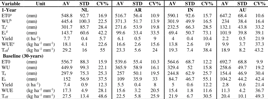
The simulated growing season ET0 using the three methods (PM, PT, and P) ranged from 786
mm for AU to 483 mm for the NL (Fig. 1a). Total season ET0 values calculated by the three
methods differed at each location (P < 0.05; Fig. 1a).
When the uncertainty of simulated WU was partitioned between Ta, Es, and ET0, and
following equations [2] to [6], the first-order sensitivity coefficient S1(Ta) contributed the most
to the variability in WU among models (Fig. 1b-d). For the single year dataset the term S1(Ta)
13
averaged over the 30-year baseline, S1(Ta), S1(Es), and S1(ET0) were 51%, 28% and 21%,
respectively (Fig. 1b). There was little change in the first order sensitivity coefficients as
temperature increased. The S1(Ta), S1(Es), and S1(ET0) values were 46, 37, and 18% at +3C
and 50, 36 and 14% at +6C (Fig. 1c). Simulations with four [CO2] showed similar results with
S1(Ta) ranging between 53 and 54% (Fig. 1d).
3.2 Observed and simulated data
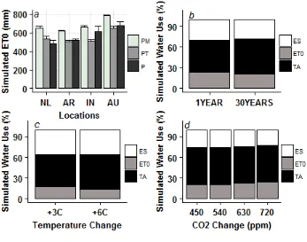
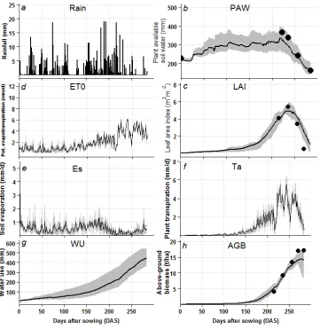
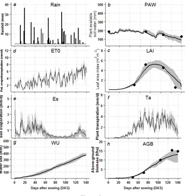
The daily patterns of growing season rainfall, observed and simulated PAW, ET0, LAI, Es,
Ta, WU, and AGB are shown for NL, AR, IN, and AU in Figs. 2-5, respectively. The four
wheat-growing locations differed in terms of the evaporative demand of the atmosphere, soil
conditions, and the temporal variability of growing season rainfall and temperature (Figs. 2-5).
For example, at AU rainfall occurred frequently throughout the season with occasional days of
heavy rainfall in spring and summer (Fig. 5a). In contrast, there was no rainfall at the IN site
(Fig. 4a). NL and AR had frequent heavy rainfall during the growing season (Figs. 2a and 3a).
The in-season observed values for the plant available soil water, aboveground biomass, water
use, and LAI were within the range of the simulations in NL, AR, and AU (Figs. 2,3, and 5).
There were some discrepancies between observed and simulated values in IN for the LAI, PAW
and WU (Fig. 4).
The end-of-season cumulative WU, WUE, Ta, Es, Teff, and Y for the single experimental year,
and for the 30-year period from 1980 to 2009 are shown in Table 1. Simulated average values for
WU was less variable than for WUE and Teff. The coefficient of variation (CV) across locations
14
for WUE. Average CV of simulated values varied between 20 and 33% for Ta, between 34 and
73% for Es, and between 24 and 55% for Teff (Table 1).
3.3 Crop simulation models sensitivity to average daily air temperature and atmospheric CO2
concentration
The average simulated WU, Y, Ta, Es, WUE, and Teff decreased with increased temperature for
all four locations (Fig. 6). However, the variability of the models increased as temperature
increased for all the variables (Fig. 6). The models showed higher uncertainties for Australia,
where except for the simulated WU which had little variability. In Australia simulated Teff varied
between -100 and +100% when temperature was increased by +6C (Fig. 6).
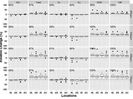
Simulated average WU, Ta, and Es decreased with increasing [CO2] while Y, WUE, and Teff
increased with increasing [CO2] at all locations (Fig. 7). The simulated relative changes to [CO2]
showed less variability than temperature. This outcome seemed to be consistent across the
models, with the exception of few outliers. At 720 compared to 360 ppm [CO2] in the four
locations, the overall simulated values changed by -4% for WU, +31% for Y, -2% for Ta, -9% for
Es, +38% for WUE, and +34% for Teff (Fig. 7). Only the variability of WUE and Teff was higher
at 720 ppm than at 360 ppm, ranging between 0 and 100% changes at 720 ppm (Fig. 7).
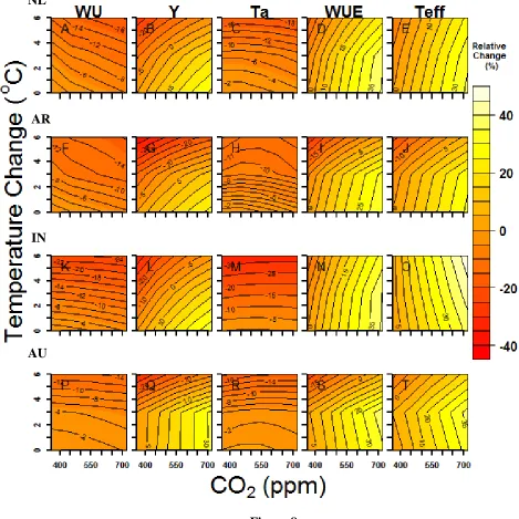
The respective effects of changing temperature and [CO2] interact in generating model
outputs of the 16 crop models. For simulated WU, increasing [CO2] to 720 ppm does not offset
its reduction caused by temperature increase (Figure 8). The effects of [CO2] in compensating
15
example, with a 6°C increase, WUE increased if [CO2] was above 450 ppm in NL and IN, or
above 550 ppm in AR and AU (Fig. 8).
Of particular interest is the variability in the direction of change in simulated responses to
increased temperature or [CO2]. It was studied by counting how many models showed similar
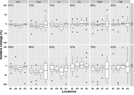
trend; for example how many models simulated a decrease in WU at +6C, and how many
simulated an increase in WU at +6C. Overall, with a 6°C increase across the four locations, 94%
of the models computed that WU decreased, 83% that Ta decreased, 52% that Es decreased, 78%
that WUE decreased, and 63% that Teff decreased (Fig. 6). Modelling the effect of 720 ppm CO2,
69% of the models agreed that WU decreased, 97% that Y increased, 56% that Ta decreased, and
83% that Es decreased. All models projected that WUE and Teff would increase (Fig. 7).
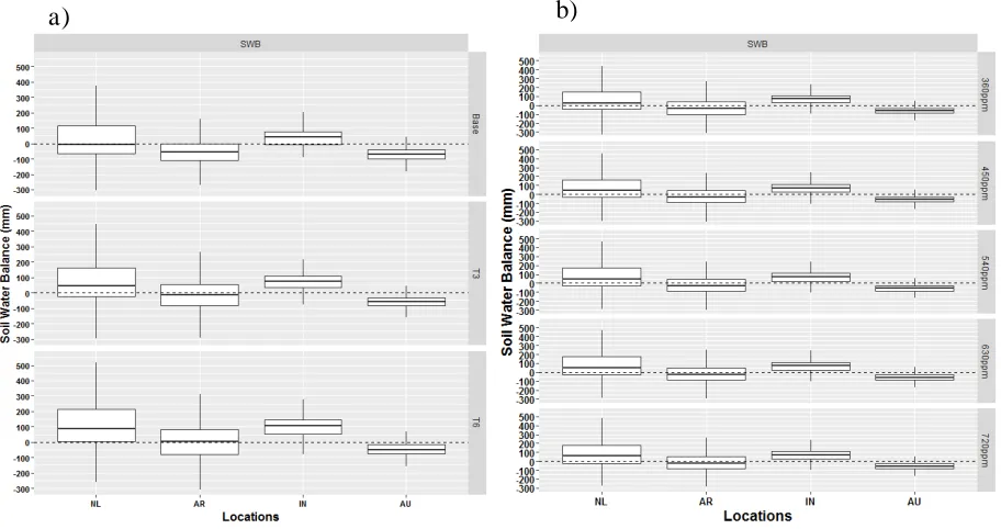
The calculated SWB using eq. [2] showed that for both baseline and sensitivity to temperature
and CO2 the NL had a higher variability among the models with respect to the other locations
(Fig. 9). The variability among the different components of eq. [2] showed that transpiration (Ta)
was the component having the higher variability followed by the drainage (Fig. 10). For
example, in the NL the simulated transpiration varied between 100 and 500 mm for the baseline
runs (No temperature changes) and drainage between 0 and 400 mm, for the upper and lower
hinge representing the 25th and 75th percentile, respectively. At +6C the variability of simulated
crop transpiration among models ranged between 10 and 540 mm while simulated drainage
ranged between 0 and 350 mm (Fig. 10a).
16
In this study, most of the variability in simulated WU was due to model differences in
and rather than the choice of the ET0 formula. This is true for the experimental years, the
30-year baseline and for the simulations with increased temperature or CO2. While differences in
the choice of the ET0 formula have been shown to be important (Kingston et al., 2009; McAfee,
2013; McKenney and Rosenberg, 1993; Utset et al., 2004; Xu and Singh, 2002), studies focusing
on the ET0 formula have not analyzed how the partitioning of ET0 between Es and Ta would
influence the simulations of crop WU. Other studies have focused on the partitioning within the
growing season of the Es and Ta only, showing that Es can account for 20% to 40% of WU
(Kool et al., 2014; French and Sculz, 1984).
Although the overall first order effect of accounted for 51% of the total of first order
effects on WU for both different temperature and CO2 changes across the four locations, no
experimental data were available to validate these aspects of the simulation. Differences among
models in simulating rooting depth/distribution and soil water extraction by roots could be an
important reason for differences in Ta estimation (Wu and Kersebaum, 2008).
Understanding the partitioning of WU between crop transpiration and soil evaporation is
critical because of its implications for agricultural, ecological, and hydrological studies. In
addition, considering the variability in the simulation of PAW, and particularly of simulated LAI,
the differences in are not surprising because the water is transpired by crops through
stomata that are on leaves.
Given the variability of the simulated SWB, and of the other components like drainage,
further research into the reasons of variation of different sub-routines among models is
necessary. The hardest part is to get detailed and accurate measurements of each sub-component
17
The large variability between models indicates that there are major differences in the way the
processes that affect water use are modeled. Differences among models in simulating soil water
extraction by roots could be an important reason for differences in Ta estimation (Wu and
Kersebaum, 2008). Variability in the simulation of PAW and LAI would have a direct effect on
the differences in Ta/ETo. Since PAW was among the given soil parameters, causes are primarily
related to differences in the models’ crop interfaces to soil (roots) and atmosphere (LAI).
Models have been tested against the same limited set of CO2 response data, which are from
open-top chamber or Free Air Carbon dioxide Enrichment Experiments (FACE) data. Models
also typically include many processes that respond to temperature, while the response to CO2 is
often lumped at a higher level of integration as discussed in details by Kersebaum and Nendel
(2014). Some models used an empirical relationship between CO2 and radiation use efficiency
while other models used the CO2 dependency of the photosynthesis light response curve
(Tubiello and Ewert, 2002) or directly simulated stomatal conductance and rubisco-kinetics
based photosynthesis.
However, there is no clear relationship between model results and model’s structure because
models are complex and many elements of structure interact with each other (Bassu et al., 2014;
Li et al., 2015; Martre et al., 2015). Further research into the sources of variation of different
sub-routines among models is necessary.
Increased [CO2] in field crops has led to decreases in WU of 3 to 8%, and an increase in Y of
8 to 31% (Hatfield et al., 2011; Kimball et al., 2002; Long et al., 2006; Manderscheid and
Weigel, 2007; Tao and Zhang, 2013). The variability in the experimental results depends on crop
management, CO2 concentrations used in the experiments, the type of experiment (e.g. open-top
18
response to CO2 concentrations across different experiments (Long, 2012). A meta-analysis of
wheat studies found that increasing [CO2] from 400 to 800 ppm increases WUE by between 5
and 38% (Hatfield et al., 2011; Kimball et al., 2002; Long et al., 2006; Manderscheid and
Weigel, 2007; Tao and Zhang, 2013; Wang et al., 2013). The results of this study regarding the
simulated response at the four locations for WU, Y, and WUE to [CO2] was in line with these
studies. This concordance contrasts with claims that on average models overestimate [CO2]
effects (Ewert et al., 2007; Long et al., 2006; Tubiello et al., 2007).
Another important outcome of our study is to have traced the average pattern of WU, WUE,
and Teff change with temperature and [CO2] increases. Despite variability, the majority of models
had the same direction of change in Y, WU, WUE, and Teff in the sensitivity to temperature and
[CO2]. This allowed us to draw conclusions about general crop responses when temperature and
[CO2] both change. The interaction between increase in temperature and increase in [CO2]
showed that, depending on the location, Y, WUE, and Teff reductions due to temperature can be
largely offset by increasing [CO2]. The response of WUE to temperature is of particular interest
since this response may be driving yield changes in many regions with limited rainfall and water
for irrigation (Pirttioja et al., 2015).
The changes in temperature used in this study (+3°C and +6°C) caused more model output
variability than the changes in atmospheric [CO2] (from 360 ppm to 720 ppm at 90 ppm
intervals). But, the crop models’ agreement related to the magnitude of changes is
variable-specific. For example, crop models showed good agreement in terms of relative change of
simulated Y under temperature and elevated [CO2] changes, WU showed good agreement under
temperature changes and lower agreement under [CO2], while WUE, and Teff showed less
19
5. Conclusion
The largest uncertainty in simulated crop WU among CSMs is due to differences in how
models simulate crop transpiration. The simulated response to increased temperature caused a
decline in WU. The sixteen models showed greatest uncertainty of simulated WUE, and Teff at
increased temperatures and with interactions between temperature and [CO2]. To improve the
simulated impacts of climate change on crop water dynamics, crop transpiration in CSMs needs
to be improved with detailed experimental data.
Acknowledgments
We thank the anonymous referees for the valuable comments and suggestions that helped
improve the manuscript.
S.G. was supported by a grant from the Ministry of Science, Research and Arts of
Baden-Württemberg (AZ Zu 33-721.3-2) and the Helmholtz Center for Environmental Research,
Leipzig (UFZ); R.P.R., T.P. and F.T. were supported by funds from the European FACCE
MACSUR project through the Finnish Ministry of Agriculture and Forestry; P.M., P.B., N.B.
and D.R. were supported by INRA Environment and Agronomy Division and by the funding
within the framework of JPI FACCE MACSUR project through the INRA Metaprogram on the
Adaptation of Agriculture and Forests to Climate Change; K.C.K. and C.N. received support
from the German Federal Office for Agriculture and Food with FACCE MACSUR
(2812ERA147) and from COST ES1106; C.M. acknowledges financial support from the
20
through the German Federal Ministry of Education and Research (BMBF); C.O.S. was supported
by the project of Regional Approaches to Climate Change for Pacific Northwest Agriculture
(REACCH-PNA) funded through award #2011-68002-30191 from the National Institute for
Food and Agriculture.
1
2
Reference
3
Alcamo, J., Florke, M. and Marker, M., 2007. Future long-term changes in global water 4
resources driven by socio-economic and climatic changes. Hydrolog Sci J, 52(2): 247-5
275. 6
Allen, R.G., Pereira, L.S., Raes, D. and Smith, M., 1998. Crop evapotranspiration: guidelines for 7
computing crop water requirements - FAO irrigation and drainage paper 56. FAO, via 8
Terme di Caracalla, Rome. 9
Angulo, C. et al., 2013. Implication of crop model calibration strategies for assessing regional 10
impacts of climate change in Europe. Agr Forest Meteorol, 170: 32-46. 11
Angus, J.F. and van Herwaarden, A.F., 2001. Increasing water use and water use efficiency in 12
dryland wheat. Agronomy Journal, 93(2): 290-298 13
Asseng, S. et al., 2013. Uncertainty in simulating wheat yields under climate change. Nature 14
Climate Change, 3(9): 827-832. 15
Asseng, S. et al., 1998. Performance of the APSIM-wheat model in Western Australia. Field 16
Crops Research, 57(2): 163-179. 17
Bassu, S. et al., 2014. How do various maize crop models vary in their responses to climate 18
change factors? Global Change Biology, 20(7): 2301-2320. 19
Blum, A., 2005. Drought resistance, water-use efficiency, and yield potential - are they 20
compatible, dissonant, or mutually exclusive? Australian Journal of Agricultural 21
Research, 56(11): 1159-1168. 22
Brisson, N., Itier, B., L'Hotel, J.C. and Lorendeau, J.Y., 1998. Parameterisation of the 23
Shuttleworth-Wallace model to estimate daily maximum transpiration for use in crop 24
models. Ecological Modelling, 107(2-3): 159-169. 25
Challinor, A.J. et al., 2014. A meta-analysis of crop yield under climate change and adaptation. 26
Nat Clim Change, 4(4): 287-291. 27
Condon, A., Richards, R., Rebetzke, G. and Farquhar, G., 2004. Breeding for high water-use 28
21
Condon, A.G., Richards, R.A., Rebetzke, G.J. and Farquhar, G.D., 2002. Improving intrinsic 30
water-use efficiency and crop yield. Crop Science, 42(1): 122-131. 31
Dixon, J., Braun, H.J. and Crouch, J., 2009. Overview: Transitioning Wheat Research to Serve 32
the Future Needs of the Developing World In: J. Dixon, H.J. Braun, P. Kosina and J. 33
Crouch (Editors), Wheat Facts and Futures 2009. CIMMYT, Mexico, D.F. 34
Elliott, J. et al., 2014. Constraints and potentials of future irrigation water availability on 35
agricultural production under climate change. P Natl Acad Sci USA, 111(9): 3239-3244. 36
Ewert, F., Porter, J.R. and Rounsevell, M.D.A., 2007. Crop models, CO2, and climate change. 37
Science, 315(5811): 459-459. 38
Foley, J.A. et al., 2011. Solutions for a cultivated planet. Nature, 478: 337-342. 39
French, R.J., Schultz, J.E., 1984. Water use efficiency of wheat in a Mediterranean-type 40
environment. I the relationship between yield, water use and climate. Australian Journal 41
of Agricultural Research, 35: 743–764. 42
Godfray, H.C.J. et al., 2010. Food Security: The Challenge of Feeding 9 Billion People. Science, 43
327(5967): 812-818. 44
Groot, J.J.R., De Willigen, P. and Verberne, E.L.J., 1991. Nitrogen turnover in the soil-crop 45
system. Developments in Plant and Soil Sciences, 44. Kluver Academic Publisher, Haren. 46
Hansen, S., 1984. Estimation of potential and actual evapotranspiration. Nordic Hydrology, 47
15(4-5): 205-212. 48
Hatfield, J.L. et al., 2011. Climate Impacts on Agriculture: Implications for Crop Production. 49
Agronomy Journal, 103(2): 351-370. 50
Howell, T.A., 2001. Enhancing water use efficiency in irrigated agriculture. Agronomy Journal, 51
93(2): 281-289. 52
Kersebaum, K.C. and Nendel, C., 2014. Site-specific impacts of climate change on wheat 53
production across regions of Germany using different CO2 response functions. European 54
Journal of Agronomy, 52: 22-32. 55
Kimball, B.A., Kobayashi, K. and Bindi, M., 2002. Responses of agricultural crops to free-air 56
CO2 enrichment. Advances in Agronomy, Vol 77, 77: 293-368. 57
Kingston, D.G., Todd, M.C., Taylor, R.G., Thompson, J.R. and Arnell, N.W., 2009. Uncertainty 58
in the estimation of potential evapotranspiration under climate change. Geophys Res Lett, 59
36. 60
Knox, J., Hess, T., Daccache, A. and Wheeler, T., 2012. Climate change impacts on crop 61
productivity in Africa and South Asia. Environ Res Lett, 7(3). 62
Kool, D. et al., 2014. A review of approaches for evapotranspiration partitioning. Agricultural 63
and Forest Meteorology, 184: 56-70. 64
Li, T. et al., 2015. Uncertainties in predicting rice yield by current crop models under a wide 65
22
Long, S.P., 2012. Virtual Special Issue on food security - greater than anticipated impacts of 67
near-term global atmospheric change on rice and wheat. Global Change Biol, 18(5): 68
1489-1490. 69
Long, S.P., Ainsworth, E.A., Leakey, A.D.B., Nosberger, J. and Ort, D.R., 2006. Food for 70
thought: Lower-than-expected crop yield stimulation with rising CO2 concentrations. 71
Science, 312(5782): 1918-1921. 72
Manderscheid, R. and Weigel, H.J., 2007. Drought stress effects on wheat are mitigated by 73
atmospheric CO2 enrichment. Agron Sustain Dev, 27(2): 79-87. 74
Martre, P. et al., 2015. Multimodel ensembles of wheat growth: many models are better than one. 75
Global Change Biology, 21(2): 911-925. 76
McAfee, S.A., 2013. Methodological differences in projected potential evapotranspiration. 77
Climatic Change, 120(4): 915-930. 78
McKenney, M.S. and Rosenberg, N.J., 1993. Sensitivity of some potential evapotranspiration 79
estimation methods to climate change. Agricultural and Forest Meteorology, 64(1-2): 81-80
110. 81
Mearns, L.O., Rosenzweig, C. and Goldberg, R., 1997. Mean and variance change in climate 82
scenarios: Methods, agricultural applications, and measures of uncertainty. Climatic 83
Change, 35(4): 367-396. 84
Monfreda, C., Ramankutty, N. and Foley, J.A., 2008. Farming the planet: 2. Geographic 85
distribution of crop areas, yields, physiological types, and net primary production in the 86
year 2000. Global Biogeochem Cy, 22(1). 87
Müller, C. and Robertson, R.D., 2014. Projecting future crop productivity for global economic 88
modeling. Agricultural Economics, 45(1): 37-50. 89
Naveen, N., 1986. Evaluation of soil water status, plant growth and canopy environemtn in 90
relation to variable water supply to wheat, Indian Agricultural Research Institute, New 91
Delhi, India. 92
Osborne, T., Rose, G. and Wheeler, T., 2013. Variation in the global-scale impacts of climate 93
change on crop productivity due to climate model uncertainty and adaptation. Agr Forest 94
Meteorol, 170: 183-194. 95
Palosuo, T. et al., 2011. Simulation of winter wheat yield and its variability in different climates 96
of Europe: A comparison of eight crop growth models. European Journal of Agronomy, 97
35(3): 103-114. 98
Passioura, J., 2006. Increasing crop productivity when water is scarce - from breeding to field 99
management. Agricultural Water Management, 80(1-3): 176-196. 100
Passioura, J.B. and Angus, J.F., 2010. Improving productivity of crops in water-limited 101
environments. Advances in Agronomy, Vol 106, 106: 37-75. 102
Penman, H.L., 1948. Natural Evaporation from Open Water, Bare Soil and Grass. Proc R Soc 103
23
Pirttioja, N., Carter, T.R., Fronzek, S., 2015. A crop model ensemble analysis of temperature and 105
precipitation effects on wheat yield across a European transect using impact response 106
surfaces. Climate Research, 65: 87–105. 107
Priestley, C. and Taylor, R.J., 1972. On the assessment of surface heat flux and evaporation 108
using large scale parameters. Monthly Weather Review, 100(2): 10. 109
Reynolds, M. and Braun, H., 2013. Achieving yield gains in wheat: Overview. In: M. Reynolds 110
and H. Braun (Editors), Proceedings of the 3rd International Workshop of the Wheat 111
Yield Consortium. CIMMYT, Obregón, Sonora, Mexico. 112
Rienecker, M.M. et al., 2011. MERRA: NASA's Modern-Era Retrospective Analysis for 113
Research and Applications. J Climate, 24(14): 3624-3648. 114
Rosenzweig, C., Jones, J.W., Hatfield, J. and Antle, J., 2011. AgMIP Protocols 115
http://www.agmip.org/agmip-protocols/, accessed July 2014. 116
Rosenzweig, C. and Parry, M.L., 1994. Potential Impact of Climate-Change on World Food-117
Supply. Nature, 367(6459): 133-138. 118
Rötter, R. and Van de Geijn, S.C., 1999. Climate change effects on plant growth, crop yield and 119
livestock. Climatic Change, 43(4): 651-681. 120
Rötter, R.P., Carter, T.R., Olesen, J.E. and Porter, J.R., 2011. Crop-climate models need an 121
overhaul. Nat Clim Change, 1(4): 175-177. 122
Rötter, R.P. et al., 2012. Simulation of spring barley yield in different climatic zones of Northern 123
and Central Europe: A comparison of nine crop models. Field Crop Res, 133: 23-36. 124
Sadras, V.O. and Angus, J.F., 2006. Benchmarking water-use efficiency of rainfed wheat in dry 125
environments. Aust J Agr Res, 57(8): 847-856. 126
Semenov, M.A., Stratonovitch, P., Alghabari, F. and Gooding, M.J., 2014. Adapting wheat in 127
Europe for climate change. J Cereal Sci, 59(3): 245-256. 128
Shen, Y.J., Ok, T., Utsumi, N., Kanae, S. and Hanasaki, N., 2008. Projection of future world 129
water resources under SRES scenarios: water withdrawal. Hydrolog Sci J, 53(1): 11-33. 130
Siebert, S. and Doll, P., 2010. Quantifying blue and green virtual water contents in global crop 131
production as well as potential production losses without irrigation. J Hydrol, 384(3-4): 132
198-217. 133
Sinclair, T.R. and Muchow, R.C., 2001. System analysis of plant traits to increase grain yield on 134
limited water supplies. Agronomy Journal, 93(2): 263-270. 135
Tao, F.L. and Zhang, Z., 2013. Climate change, wheat productivity and water use in the North 136
China Plain: A new super-ensemble-based probabilistic projection. Agr Forest Meteorol, 137
170: 146-165. 138
Taylor, S.L., Payton, M.E. and Raun, W.R., 1999. Relationship between mean yield, coefficient 139
of variation, mean square error, and plot size in wheat field experiments. Commun Soil 140
Sci Plan, 30(9-10): 1439-1447. 141
Tebaldi, C. and Knutti, R., 2007. The use of the multi-model ensemble in probabilistic climate 142
24
Tilman, D., Balzer, C., Hill, J. and Befort, B.L., 2011. Global food demand and the sustainable 144
intensification of agriculture. P Natl Acad Sci USA, 108(50): 20260-20264. 145
Travasso, M.I., Magrin, G.O., Rodriguez, R. and Grondona, M.O., 1995. Comparing CERES-146
Wheat and SUCROS2 in the Argentinean Cereal Region. In: A. Zerger and R.M. Argent 147
(Editors), Internationa Congress on Modelling and Simulation. Modelling and Simulation 148
Society of Australia and New Zealand, The University of Newcastle, Newcastle, NSW, 149
pp. 366-369. 150
Tubiello, F.N. et al., 2007. Crop response to elevated CO2 and world food supply - A comment 151
on "Food for Thought..." by Long et al., Science 312 : 1918-1921, 2006. Eur J Agron, 152
26(3): 215-223. 153
Tubiello, F.N. and Ewert, F., 2002. Simulating the effects of elevated CO2 on crops: approaches 154
and applications for climate change. European Journal of Agronomy, 18(1-2): 57-74. 155
Utset, A., Farre, I., Martinez-Cob, A. and Cavero, J., 2004. Comparing Penman-Monteith and 156
Priestley-Taylor approaches as reference-evapotranspiration inputs for modeling maize 157
water-use under Mediterranean conditions. Agricultural Water Management, 66(3): 205-158
219. 159
Wang, L., Feng, Z.Z. and Schjoerring, J.K., 2013. Effects of elevated atmospheric CO2 on 160
physiology and yield of wheat (Triticum aestivum L.): A meta-analytic test of current 161
hypotheses. Agr Ecosyst Environ, 178: 57-63. 162
White, J.W., Hoogenboom, G., Kimball, B.A. and Wall, G.W., 2011a. Methodologies for 163
simulating impacts of climate change on crop production. Field Crop Res, 124(3): 357-164
368. 165
White, J.W., Hoogenboom, G., Wilkens, P.W., Stackhouse, P.W. and Hoel, J.M., 2011b. 166
Evaluation of Satellite-Based, Modeled-Derived Daily Solar Radiation Data for the 167
Continental United States. Agron J, 103(4): 1242-1251. 168
Wu, L. and Kersebaum, K.C., 2008. Modeling water and nitrogen interaction responses and their 169
consequences in crop models. In: L.R. Ahuja, V.R. Reddy, S.A. Saseendran and Q. Yu 170
(Editors), Response of crops to limited water: understanding and modeling water stress 171
effects on plant growth processes. Advances in Agricultural Systems Modeling. ASA, 172
CSSA, SSSA, Madison, WI, USA, pp. 215-249. 173
Xu, C.Y. and Singh, V.P., 2002. Cross comparison of empirical equations for calculating 174
potential evapotranspiration with data from Switzerland. Water Resources Management, 175
16(3): 197-219. 176
25
Table 1. Average (AV), standard deviation (STD), and coefficient of variability (CV%) for the
Netherlands (NL), Argentina (AR), India (IN), and Australia (AU) for seven parameters using
the 16 crop simulation models.
Variable Unit AV STD CV% AV STD CV% AV STD CV% AV STD CV%
1-Year NL AR IN AU
ET0a (mm) 548.8 92.7 16.9 516.7 56.4 10.9 590.1 92.6 15.7 647.2 68.4 10.6
WUb
(mm) 445.4 100.3 22.5 371.3 51.7 13.9 301.9 49.9 16.5 234 38.4 16.4 Tac (mm) 301.7 85.7 28.4 271.6 53.9 19.8 232.5 66.3 28.5 132.1 43.8 33.2
Esd (mm) 143.7 60.6 42.2 99.6 33.4 33.5 69.4 50.7 73.1 101.9 39.8 39.1
Yield (t ha-1) 7.7 0.4 5.7 6.1 0.5 9 4 0.4 10.4 2.2 0.5 21.9
WUEe
(kg ha-1
mm-1
) 18.1 4.1 22.6 16.6 2.6 15.6 13.8 2.6 19 9.9 3.7 37.3 Tefff (kg ha-1 mm-1) 29.2 16 55 23.3 5.6 24 19.3 7.4 38.4 18.9 8.2 43.2
Baseline (30-years)
ET0 (mm) 556.7 88.3 15.9 539.6 55.4 10.3 564.6 68.7 12.2 692.7 68.8 9.9 WU (mm) 449.9 99.3 22.1 365.9 58.9 16.1 329.4 52 15.8 258.6 49.7 19.2 Ta (mm) 297.9 75.3 25.3 257 50.1 19.5 244.8 62.9 25.7 154.4 46.9 30.4
Es (mm) 152 56.9 37.5 109 35.9 33 84.7 46.7 55.1 104.2 44.2 42.4
Yield (t ha-1) 7.4 0.9 12.3 5.5 0.4 8 5 0.6 12.2 2.8 0.6 21.4
WUE (kg ha-1
mm-1
) 17.3 4.9 28.1 15.6 3.2 20.5 15.4 1.8 11.6 11.3 4.2 36.7 Teff (kg ha-1 mm-1) 27.5 13.4 48.6 22.5 5.8 25.9 21.9 6.7 30.5 20.4 10.1 49.3 a
Potential evapotranspiration; b
Water use; c
Crop transpiration; d
Soil evaporation; e
Water use efficiency; f
26
Figure Caption
Figure 1. Simulated potential reference evapotranspiration (ET0) and percentage of simulated
water use variance. (a) Simulated seasonal ET0 for the 30-year baseline calculated from the
average of those models using Penman-Monteith (PM, 7 models), Priestley-Taylor (PT, 6
models), and Penman (P, 3 models) equations. Different letters indicate significant differences at
= 0.05. (b-d) Simulated proportion of variance for water use explained by ET0 (light grey),
crop transpiration (Ta; black), and soil evaporation (Es; white) for (b) the experimental year and
the 30-year baseline, (c) average daily air temperature increases, and (d) increasing atmospheric
CO2 concentrations.
Figure 2. Daily variability in plant water use and crop growth-related variables for an
experimental site in the Netherlands (NL). (a) Daily growing season rainfall. (b-h) Average of 16
crop models (black line) with the interval between the 20th and 80th percentiles (shaded grey area) for plant available water (PAW), daily potential evapotranspiration (ET0), leaf area index (LAI),
soil evaporation (Es), plant transpiration (Ta), water use (WU), and aboveground biomass
(AGB). Observed values (closed symbols) are shown for plant available soil water, LAI, and
above-ground biomass.
Figure 3. Daily variability in plant water use and crop growth-related variables for an
experimental site in Argentina (AR). (a) Daily growing season rainfall. (b-h) Average of 16 crop
models (black line) with the interval between the 20th and 80th percentiles (shaded grey area) for plant available water (PAW), daily potential evapotranspiration (ET0), leaf area index (LAI), soil
evaporation (Es), plant transpiration (Ta), water use (WU), and aboveground biomass (AGB).
Observed values (closed symbols) are shown for plant available soil water, LAI, and
above-ground biomass.
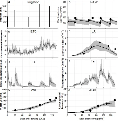
Figure 4. Daily variability in plant water use and crop growth-related variables for an
experimental site in India (IN). (a) Irrigation. (b-h) Average of 16 crop models (black line) with
the interval between the 20th and 80th percentiles (shaded grey area) for plant available water
(PAW), daily potential evapotranspiration (ET0), leaf area index (LAI), soil evaporation (Es),
plant transpiration (Ta), water use (WU), and aboveground biomass (AGB). Observed values
(closed symbols) are shown for plant available soil water, LAI, water use, and above-ground
27
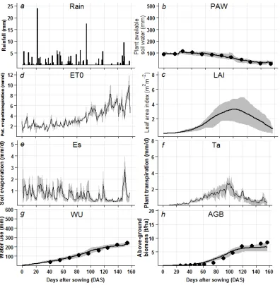
Figure 5. Daily variability in plant water use and crop growth-related variables for an
experimental site in Australia (AU). (a) Daily growing season rainfall. (b-h) Average of 16 crop
models (black line) with the interval between the 20th and 80th percentiles (shaded grey area) for plant available water (PAW), daily potential evapotranspiration (ET0), leaf area index (LAI), soil
evaporation (Es), plant transpiration (Ta), water use (WU), and aboveground biomass (AGB).
Observed values (closed symbols) are shown for plant available soil water, water use, and
above-ground biomass.
Figure 6. Effects of higher temperatures, respect to the 30 years historical data, on simulated
water use related variables and grain yield. Boxplot of the relative change of multi-model
simulations with increases in average daily air temperature of 3°C and 6°C for water use (WU),
grain yield (Y), cumulative crop transpiration (Ta), cumulative soil evaporation (Es), water use
efficiency (WUE), and transpiration efficiency (Teff), for experimental sites in the Netherlands
(NL), Argentina (AR), India (IN), and Australia (AU). The percentage of individual models that
predict the same trend is shown above each set of points.
Figure 7. Effects of increases in atmospheric CO2 concentrations on simulated water use related
variables and grain yield. Boxplot of the relative change of multi-model simulation with
increased atmospheric CO2 concentrations for water use (WU), grain yield (Y), cumulative crop
transpiration (Ta), cumulative soil evaporation (Es), water use efficiency (WUE), and
transpiration efficiency (Teff), for experiment sites in the Netherlands (NL), Argentina (AR),
India (IN), and Australia (AU). The percentage of individual models that predict the same trend
as the multi-model mean is shown above each set of points.
Figure 8. Interaction patterns between temperature and atmospheric CO2 concentration on
simulated water use related variables and grain yield. Relative change in (a, f, k, and p) water use
(WU), (b, g, l, and q) grain yield (Y), (c, h, m, and r) cumulative crop transpiration (Ta), (d, i, n,
and s) water use efficiency (WUE), and (e, j, o, and t) transpiration efficiency (Teff) simulations
for experimental sites in (a-e) the Netherlands, (f-j) Argentina, (k-o) India, and Australia (p-t)
with increases in average daily air temperature versus atmospheric CO2 concentration.
Figure 9. Boxplots of the simulated Soil Water Balance (SWB) calculated using eq. [2] for the
Netherlands (NL), Argentina (AR), India (IN), and Australia (AU); (a) Effect of temperature on
28
daily air temperature of 3°C (T3) and 6°C (T6); (b) for the increases in atmospheric CO2
concentrations.
Figure 10. Boxplots of the simulated components of the Soil Water Balance (SWB) calculated
using eq. [2]. Simulated Drainage (Drain), Runoff (Runoff), crop transpiration (Ta), and soil
evaporation (Es) are shown for the Netherlands (NL), Argentina (AR), India (IN), and Australia
(AU); (a) Effect of temperature on each of the model simulation of the baseline 30-years period
(Base), the increases in average daily air temperature of 3°C (T3) and 6°C (T6); (b) for the
29
30
[image:31.612.116.477.73.444.2]31
[image:32.612.117.500.73.475.2]32
[image:33.612.116.495.76.468.2]33
34
35
36
Figure 8. NL
AR
IN
37
Figure 9.
38
Figure 10.
39 SUPPLEMENTAL INFORMATION
Table S1. Field experiments, crop management and climate characteristics of the four sites where models were
calibrated modified after Asseng et al. (2013).
Experiment
Location Wageningen Balcarce New Delhi Wongan Hills
Country The Netherlands Argentina India Australia
Latitudea 51.97 -37.5 28.38 -30.89
Longitudea 5.63 -58.3 77.12 116.72
Environment High-yielding
long-season
High/medium-yielding medium-season
Irrigated short-season
Low-yielding rain-fed
short-season Soils
Soil type Silty clay loam Clay loam Sandy loam Loamy sand
Maximum root depth (cm) 200 130 160 210
Plant available soil water content (mm to
maximum rooting depth) 354 205 121 125
Crop management
Cultivar Arminda Oasis HD 2009 Gamenya
Sowing date (day of year) 294 223 328 164
Total applied N fertilizer (kg N ha-1) 160 120 120 50
Total irrigation (mm) 0 0 383 0
Phenology
Anthesis (day of year) 178 328 49 275
Maturity (day of year) 213 363 93 321
Growing Season Length (days) 284 140 130 157
Environmental Characteristics
Experimental year 1982/1983 1992 1984/1985 1984
Mean growing season air temperature (°C) 8.8 13.7 17.3 14.0
Mean growing season rainfall (mm) 595 336 0 164
30 years average 1981-2010 1981-2010 1981-2010 1981-2010
Mean growing season air temperature (°C) 8.5 12.0 18.9 16.2
Mean growing season rainfall (mm) 716 395 84 246
a
Geographical degrees and minutes – the latter expressed in decimals; the minus sign before latitude and
40
Table S2. Soil depth, hydraulic limits, bulk density, organic carbon, and soil pH provided to the modelling group
for each site.
Location Depth LL DUL SAT BD OC pH
(cm) (cm3 cm-3) (cm3 cm-3) (cm3 cm-3) (g cm-3) (%)
the Netherlands 5 0.18 0.39 0.49 1.35 2.80 6
10 0.18 0.39 0.49 1.35 2.80 6
20 0.18 0.39 0.49 1.35 2.80 6
30 0.18 0.39 0.49 1.35 2.80 6
40 0.18 0.37 0.49 1.35 1.40 6
60 0.20 0.37 0.49 1.35 1.40 6
80 0.20 0.37 0.49 1.35 1.20 6
100 0.20 0.37 0.49 1.35 1.20 6
130 0.20 0.37 0.49 1.35 1.00 6
200 0.20 0.37 0.49 1.35 1.00 6
Argentina 5 0.16 0.38 0.47 1.05 3.15 6.2
20 0.17 0.35 0.45 1.10 3.30 5.9
40 0.18 0.36 0.43 1.15 1.20 6.0
60 0.18 0.38 0.48 1.30 0.70 6.4
80 0.26 0.40 0.49 1.35 0.30 6.6
100 0.14 0.30 0.40 1.30 0.10 6.5 120 0.14 0.30 0.40 1.30 0.10 6.5
India 15 0.11 0.17 0.37 1.56 0.45 7.9
30 0.11 0.17 0.37 1.59 0.35 8.0
60 0.11 0.18 0.37 1.50 0.31 8.0
90 0.11 0.18 0.37 1.50 0.20 8.2
120 0.12 0.19 0.37 1.55 0.19 8.5 150 0.12 0.19 0.37 1.54 0.19 8.6 180 0.12 0.19 0.37 1.58 0.19 8.6
Australia 5 0.07 0.13 0.35 1.31 1.23 4.70
41
Table S3. Modeling approaches of 26 wheat simulation models used in this study, modified after Asseng et al. (2013).
Model L
ea f a re a / lig ht inte rc ept io n a L ig ht utiliza tio n b Yield f o rma tio n c P heno lo g y d Ro o t dis tributio n o v er depth e E nv iro nm e nta l co ns tra ints inv o lv ed f T y pe o f wa ter s tre ss g T y pe o f hea t st re ss h Wa ter dy na mics i E v a po tra ns pira tio n j So il CN -mo del k P ro ce ss mo dified by elev a ted CO 2 l No . cult iv a r pa ra met er s Clima te inp ut v a ria bles m M o del r ela tiv e n M o del t y pe o
APSIM-Nwheat S RUE Prt T/DL/V EXP W/N/A S V C PT CN/P(3)/B RUE/TE 7 R/Tx/Tn/Rd C P
APSIM-wheat S RUE Prt/Gn/B T/DL/V/O O W/N/A E - C/R PT/PM CN/P(3)/B RUE/TE /CLN
7 R/Tx/Tn/Rd/e/W C P
AquaCrop S TE HI/B T/DL/V/O EXP W/N/H E/S V/R C FAO
PM
none TE 2 R/Tx/ETo none P
CropSyst S TE/RUE HI/B T/DL/V EXP W/N/H E R C/R PM N/P(4) TE/RUE 16 R/Tx/Tn/Rd/RH/W none P
DSSAT-CROPSIM-CERES S RUE B/Gn T/DL/V EXP W/N E/S - C PT CN/P(4)/B RUE/TE 7 R/Tx/Tn/Rd/RH/W C P DSSAT-CROPSIM S RUE Prt T/DL/V LIN W/N E/S V C PT CN/P(4)/B RUE/TE 21 R/Tx/Tn/Rd/ none p
EPIC wheat S RUE HI T/V EXP W/N/H E V C P/PM/P
T/HAR
N/P(5)/B RUE/TE /GY
16 R/Tx/Tn/Rd/RH/W E P
Expert-N – CERES S RUE B/Gn T/DL/V EXP W/N E/S - R PM CN/P(3)/B RUE 7 R/Tx/Tn/Rd/RH/W C P
Expert-N – GECROS D P-R/TE Gn/Prt T/DL/V EXP W/N E/S - R PM CN/P(3)/B RUE/TE 10 R/Tx/Tn/Rd/RH/W S P
Expert-N – SPASS D P-R Gn/Prt T/DL/V EXP W/N E/S - R PM CN/P(3)/B RUE 5 R/Tx/Tn/Rd/RH/W C/S P
Expert-N – SUCROS D P-R Prt T EXP W/N E/S - R PM CN/P(3)/B RUE 2 R/Tx/Tn/Rd/RH/W S P
FASSET D RUE HI/B T/DL EXP W/N E/S - C MAK CN/P(6)/B RUE 14 R/Tx/Tn/Rd none P
GLAM-Wheat S RUE/TE B/HI T/DL/V LIN W/H E R C PT none RUE/TE 22 R/Tx/Tn/Td/Ta/e none G
HERMES D P-R Prt T/DL/V/O EXP W/N/A E/S - C PM/TW
/PT
N/P(2) RUE/F 6 R/Tx/Tn/Rd/e/RH/W S/C P
InfoCrop D RUE Prt/Gn T/DL EXP W/N/H E V/R C PM/PT CN/P(2)/B RUE/TE 10 R/Tx/Tn/Rd/W/E S P
LINTUL-4 D RUE Prt/B T/DL LIN W/N/A E - C P N/P(0)/-* RUE/TE 4 R/Tx/Tn/Rd/e/W L P
LINTUL -FAST D RUE Prt T/DL/V EXP W E C P CN/P(3) RUE/TE 4 R/Tx/Tn/Rd/RH L P
LPJmL S P-R HI_mws/B T/V EXP W E - C PT none F 3 R/Ta/Rd/Cl E G
42
MONICA S RUE Prt T/DL/V/O EXP W/N/A/H E V C PM CN/P(6)/B F 15 R/Tx/Tn/Rd/RH/W S/C P
[image:43.792.7.768.71.219.2]O’Leary-model S TE Gn/Prt T/DL SIG W/N/H E/S V C P N/P(3)/B TE 18 R/Tx/Tn/Rd/RH/W none P
Table A2. Continued
SALUS S RUE Prt/HI T/DL/V EXP W/N/H E V C PT CN/P(3)/B
(2)
RUE 18 R/Tx/Tn/Rd C P
Sirius D RUE B/Prt T/DL/V EXP W/N E - C P/PT N/P(2) RUE 14 R/Tx/Tn/Rd/e/W P
SiriusQuality D RUE B/Prt T/DL/V EXP W/N S - C P/PT N/P(2) RUE 14 R/Tx/Tn/Rd/e/W I P
STICS D RUE Gn/B T/DL/V/O SIG W/N/H E/S V/R C P/PT/S
W
N/P(3)/B RUE/TE 15 R/Tx/Tn/Rd/e/W C P
WOFOST D P-R Prt/B T/DL LIN W/N* E/S - C P P(1) RUE/TE 3 R/Tx/Tn/Rd/e/W S G
a S, simple approach (e.g. LAI); D, detailed approach (e.g. canopy layers).
b RUE, radiation use efficiency approach; P-R, gross photosynthesis – respiration; TE, transpiration efficiency biomass growth.
c HI, fixed harvest index; B, total (above-ground) biomass; Gn, number of grains; Prt, partitioning during reproductive stages; HI_mw, harvest index modified by
water stress.
d T, temperature; DL, photoperiod (day length); V, vernalization; O, other water/nutrient stress effects considered. e LIN, linear, EXP, exponential, SIG, sigmoidal, Call, carbon allocation; O, other approaches.
f W, water limitation; N, nitrogen limitation; A, aeration deficit stress; H, heat stress. g E, actual to potential evapotranspiration ratio; S, soil available water in root zone. h V, vegetative organ (source); R, reproductive organ (sink).
i C, capacity approach; R, Richards approach.
j P, Penman; PM, Penman-Monteith; PT, Priestley –Taylor; TW, Turc-Wendling; MAK, Makkink; HAR, Hargreaves; SW, Shuttleworth and Wallace (resistive
model), (“bold” indicates approached used during the study).
kCN, CN model; N, N model; P(x), x number of organic matter pools; B, microbial biomass pool.
l RUE, radiation use efficiency; TE, transpiration efficiency; GY, grain yield; CLN, critical leaf N concentration; F, Farquhar model.
m Cl, cloudiness; R, rainfall; Tx, maximum daily temperature; Tn, minimum daily temperature; Ta, average daily temperature; Td, dew point temperature; Rd,
radiation; e, vapor pressure; RH, relative humidity; W, wind speed.
n C, CERES; L, LINTUL; E, EPIC; S, SUCROS; I, Sirius.
o P, point model; G, global or regional model (regarding the main purpose of model).