i ABSTRACT
ii ABSTRAK
iii
ACKNOWLEDGEMENTS
First and above all, I praise Allah the almighty for providing me this opportunity and granting me the capability to proceed successfully.
This project appears in its current form due to the assistance and guidance of several people. Special appreciation goes to my supervisor, Dr. Md Fahmi bin Abd Samad @ Mahmood, for his relentless support, thoughtful guidance and correction of the project. I attribute the level of my bachelor degree to his encouragement and effort and without him, this project would not have been completed or written. One simply could not wish for a better or friendlier supervisor. I am grateful to Dr. Mohd Basri Bin Ali for his encouragement and practical advice. I am also thankful to him for reading my reports, commenting on my views and helping me understand and enrich my ideas. My thanks also go to Dr Siti Hajar for providing many valuable comments that improved the presentation and contents of this dissertation.
My deepest gratitude goes to my beloved parents, Mr. Hj Mohd Rafie bin Hj Tibek and Mrs. Hjh Noorafizah bt Abdul Aziz for their material and spiritual support in all aspects of my life. Thank you both for giving me strength to reach for the stars and chase my dreams. I also would like to thank to all my siblings for their endless love, prayers and encouragement. I am particularly grateful to my sweetheart for his devoted support throughout my study.
Last but not least, thanks to all my close friends Nurfa bt Fahar and Siti Nur Ariffah Alia for the joyful gatherings and all their supports. I deeply appreciate to all my friends that helped me stay through these difficult years. Their support and care helped me overcome setbacks and stay focused on my graduate study. I greatly value their friendship. To those who indirectly contributed in this research, your kindness means a lot to me. Thank you very much.
iv
TABLE OF CONTENTS
ABSTRACT _______________________________________________________________ i ACKNOWLEDGEMENTS __________________________________________________ iii TABLE OF CONTENTS ____________________________________________________ iv LIST OF TABLE __________________________________________________________ vii LIST OF FIGURES _______________________________________________________ viii LIST OF ABBREVIATIONS ________________________________________________ xii LIST OF SYMBOLS/NOTATIONS _________________________________________ xiii
CHAPTER ONE ____________________________________________________________ 1 INTRODUCTION __________________________________________________________ 1
v
vi
vii
LIST OF TABLE
TABLE TITLE PAGE
2.1 Differences between white box, gray box and back box models 8
3.1 MATLAB windows 19
3.2 Result of arx441 and iv441 model 46
4.1 Model estimation and validation result for first equation 63 4.2 Parameter values for first equation 64 4.3 Summarize model estimation and validation results for second
equation
71
4.4 Parameter values for second equation 72 4.5 Summarize model estimation and validation results for third
equation
76
viii
LIST OF FIGURES
FIGURE TITLE PAGE
2.1 The system identification loop 5
2.2 Estimation of parameters of a mathematical model from timeseries of the input variable and the output variable
13
3.1 The default view of MATLAB desktop 19 3.2 The main ―ident‖ information window 21 3.3 The different areas in the System Identification application 21
3.4 Import Data dialog box 22
3.5 Import Data window 23
3.6 System Identification Tool GUI with icon named Dryer 24
3.7 List preprocess commands 25
3.8 New Dataset 25
3.9 Mean-centered dataset (dryerd) for working and validation data 26
3.10 Estimate menu window 27
3.11 Parametric model window 27
ix
3.13 Linear parametric models window 29
3.14 Order editor window. 29
3.15 Model view palette after estimate model 30
3.16 Residual analysis 31
3.17 Zeros and Poles window 32
3.18 Step response plot 33
3.19 Impulse response plot 33
3.20 Model output plot 34
3.21 Noise spectrum window 35
3.22 Quantitative diagnostic window 35
3.23 Summary in MATLAB window 36
3.24 IV method in linear parametric model window 37
3.25 System identification window 37
3.26 Analysis of arx441 and iv441 autocorrelation plot 38 3.27 Analysis of arx441 and iv441 poles and zeros plot 39 3.28 Analysis of arx441 and iv441 step response plot 40 3.29 Zoom in analysis of arx441 and iv441 step response plot 41 3.30 Analysis of arx441 and iv441 model output plot 42 3.31 Analysis of arx441 and iv441 noise spectrum plot 43
3.32 Information of arx441 model 44
x
3.34 Editor window 48
3.35 Click Debug>>Run (F5) at Editor window 49
3.36 Figure 1 window 49
3.37 Command Window 50
3.38 System Identification Tool window 50
3.39 Import Data dialog box 51
3.40 Import Data window 52
3.41 Sim1 data had been imported to the data board 53
3.42 Time Plot 53
3.43 Linear Parametric Models and Order Editor window for Least Square method
55
3.44 System Identification window with arx352 model 55 3.45 System Identification window with arx352, arx322 and arx382
models
56
3.46 System Identification window with arx352, arx322, arx382, iv352, iv322 and iv382 models
57
4.1 Analysis of model output plot for first equation 61 4.2 Residuals analysis for first equation 62
4.3 Data Information of arx352 model 63
[image:10.612.82.494.65.717.2]xi
xii
LIST OF ABBREVIATIONS
AR - AutoRegressive
ARMAX - AutoRegressive Moving Average with eXogenous input ARX - AutoRegresive with eXogenous input
FPE- Final Prediction Error GUI - Graphical User Interface IV- Instrumental Variable LS - Least squares
MATLAB- Matrix Laboratory NAR - Nonlinear AutoRegressive
NARMAX - Nonlinear AutoRegressive Moving Average with eXogenous input NARX - Nonlinear AutoRegresive with eXogenous input
xiii
LIST OF SYMBOLS/NOTATIONS
^
= Estimated parameter vector = Matrix regressor
M
=Model set
2
=Constant variance = Constraints = Parameter vector
M
D =Open subset
1
CHAPTER ONE
INTRODUCTION
1.1 Background Study
2
model structure in order to fit the model output to measured system output data. The fitting can be done either manually by graphical methods, or by having a computer perform an optimization procedure. In this project, fit the model will be performed using GUI ‗ident‘ in MATLAB. Parameter is a set of methods to obtain a physical model of a dynamic system from experimental data. In this project will explore the various existing methods of parameter estimation but more focused on instrumental variable and least square method. Both methods are based on a prediction model structure which is linearly parameter.
1.2 Problem Statement
3
output data. While, instrumental variable method has ability to counteract the effects of a more general class of noise signals. For more detailed information, the difference between least square and instrumental variable will be discussed in Chapter 3.
1.3 Objective
There are an objectives that need to be achieved at the end of this project, which are:
i) To perform system identification using linear differential equation model.
ii) To investigate the performance of difference parameter estimation method in identification.
1.4 Scope of Project
The scope of this project are:
i) Identification will be performed using GUI ‗ident‘ in MATLAB.
ii) Model to be used is autoregressive with exogeneous input (ARX) model.
4
CHAPTER TWO
LITERATURE REVIEW
2.1 System Identification
5
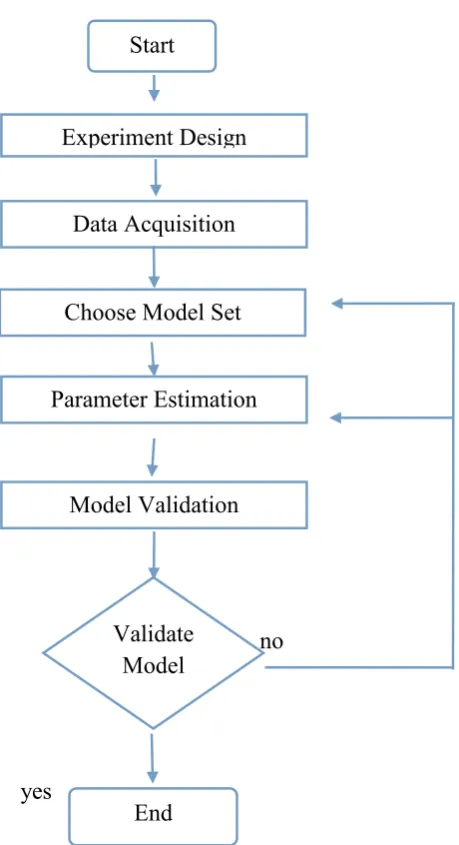
(Abd Samad,2014). The third step in system identification is the parameter estimation where the estimations of parameters taking into account the selected model structure are assessed. The fourth step is the model validity tests expected to confirm or validate the representation of the last model chose. The flow chart is given as Figure 2.1.
no
[image:18.612.213.443.216.639.2]yes
Figure 2.1: The system identification loop Experiment Design
Data Acquisition
Choose Model Set
Parameter Estimation
Model Validation
Validate Model
6 2.2 Mathematical Modeling
Mathematical models of natural and man-made systems play an essential role in today‘s science and technology. Mathematical model is a portrayal of a system utilizing mathematical concepts and language. Mathematical modeling is the process of developing a mathematical model. Choosing a suitable model structure is important procedure before its estimation. The choise of model structure is based upon comprehension of the physical systems.
2.2.1 Types of Mathematical Models
A model is a mathematical representation of a physical, biological or data system. Models permit us to reason about a system and make predictions about how a system will act. There are a variety of model structures available to assist in modeling a system. There are three main types of models are common in system identification: theoretical or white-box model, empirical or black-box model and semi-empirical or gray-box model. System identification methods can deal with an extensive variety of system dynamics without knowledge of the actual system physics,there by lessening the designing exertion required to create models.
2.2.1.1 Theoretical or White-box Identification
7
priori knowledge dominates the model. The strength of this box identification is that it will permit the user to endeavor invariant prior knowledge.
2.2.1.2 Empirical or Black box Identification
An assortment of parametric model structures are accessible to help in modeling an unknown system. Parametric models despict systems in terms of differential equations and transfer functions. These models give understanding into the system physics and compact model structures. It is often valuable to test a various structures to decide the best one. A parametric model structure is otherwise called a black-box model. The black box is an abstract class that represents a concrete open system that can be viewed purely in terms of stimulus input and output reaction. Both model structure and parameter are determined from experimental modeling. For building black box model, no or very little prior knowledge is exploited. The model parameters have no direct relationship to first principle.
2.2.1.3 Gray box Identification
8
2.2.1.4 Comparison of White Box, Black Box and Gray Box Model.
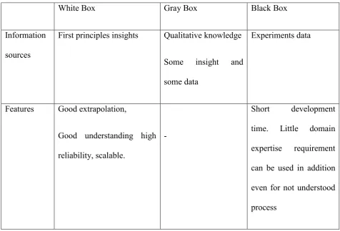
[image:21.612.78.555.333.657.2]Table 2.1 gives an overview of the differences between these modeling approaches. The blank fields for gray box models can be almost any combination of white and black box models. The advantages and drawbacks of gray box models lie somewhere between white and black box models, make them a good compromise in practice.
Table 2.1: Differences between white box, gray box and back box models.
White Box Gray Box Black Box
Information sources
First principles insights Qualitative knowledge
Some insight and some data
Experiments data
Features Good extrapolation,
Good understanding high reliability, scalable.
-
9 Drawbacks Time consuming, detailed
domain expertise requirement knowledge restricts accuracy only for well understood process.
-
No reliable extrapolation,
Not scalable,
Data restricts accuracy,
Little understanding
Application areas
Planning, construction, design rather simple processes
-
Only for existing processes rather complex processes
2.2.2 Classification of Mathematical Models
Mathematical models may be classified according to their structure and nature. Thus, mathematical models may be linear or non-linear, static or dynamic,deterministic or stochastic and discrete or continuous.
10
to vary throughout the course of a simulation run, and its utilization gets to be vital where interdependencies between parameter cannot be considered.
Static or Dynamic, according to the time variations in the system are not or are taken into account. A static model or steady-state model computes the system in equilibrium, and along these lines is time-invariant. A static model cannot be changed, and one cannot enter alter mode when static model is open for detail view. A dynamic model covers for time-dependent changes in the state of the system. Dynamic models are normally represented by differential equations.
Deterministic or Stochastic, as indicated by the chance variables are not or are considered. A deterministic model is one in which each arrangement of variable states is uniquely determined by parameters in the model and by sets of past states of these variables. Deterministic models depict conduct on the basic of some physical laws. A stochastic model is one where exact prediction is impractical and irregularity is present and variable states are not described by unique values, but rather by probability distributions.
11
All dynamic system models may be isolated into two major types based on whether
they characterize a continuous-time or discrete-time process (Unbehauen and Rao, 1987). Much of the current literature on identification is currently worried with the identification of continuous-time models (Subrahmanyam, 1993). Furthermore, for many applications, continuous time models are more appealing to engineers than discrete-time models on the grounds that they are closely related to the underlying physical systems, while discrete-time model is considered to be defined at a sequence of time-instants related to measurement. In other hand, the most common classification of models is based on whether the model represents time-varying or time-invariant systems. For time-invariant systems, difference equation models are normally preferred. For time-varying systems, among prominent choices are cascaded block model, neural network, wavelet network and cellular automata (Abd Samad,2014). In difference equation it can be separated into linear and nonlinear models. For linear difference equation model, ARX (Average Model with eXternal input), ARMAX (AutoRegressive Moving Average with eXogenous input) and Output-Error model (OE) are the most used model. While examples of nonlinear difference equation model include NARX (Nonlinear AutoRegressive with eXogenous input), NARMAX (Nonlinear ARMAX) and NOE (Nonlinear Output Error) models.
Since the system identification handles a wide variety of different model structures, it is important that these can be defined in a flexible way. For ARX model, the most used model structure is the simple linear difference equation is (Paktos and Fassois, 2003):
) 1 ( ... ) ( ) ( ... ) 1 ( )
(t a1y t a y tna b1u tnk b u tnknb