Modelling subject-specific childhood growth using linear mixed-effect models with cubic regression splines.

RESEARCH ARTICLE

Modelling subject-specific childhood

growth using linear mixed-effect models

with cubic regression splines

Laura M. Grajeda

_{, Andrada Ivanescu}

_{, Mayuko Saito}

_{, Ciprian Crainiceanu}

_{, Devan Jaganath}

_,

Robert H. Gilman

_{, Jean E. Crabtree}

_{, Dermott Kelleher}

_{, Lilia Cabrera}

_{, Vitaliano Cama}

and William Checkley

Abstract

Background: Childhood growth is a cornerstone of pediatric research. Statistical models need to consider individual trajectories to adequately describe growth outcomes. Specifically, well-defined longitudinal models are essential to characterize both population and subject-specific growth. Linear mixed-effect models with cubic regression splines can account for the nonlinearity of growth curves and provide reasonable estimators of population and subject-spe-cific growth, velocity and acceleration.

Methods: We provide a stepwise approach that builds from simple to complex models, and account for the intrinsic complexity of the data. We start with standard cubic splines regression models and build up to a model that includes subject-specific random intercepts and slopes and residual autocorrelation. We then compared cubic regression splines vis-à-vis linear piecewise splines, and with varying number of knots and positions. Statistical code is provided to ensure reproducibility and improve dissemination of methods. Models are applied to longitudinal height measure-ments in a cohort of 215 Peruvian children followed from birth until their fourth year of life.

Results: Unexplained variability, as measured by the variance of the regression model, was reduced from 7.34 when using ordinary least squares to 0.81 (p < 0.001) when using a linear mixed-effect models with random slopes and a first order continuous autoregressive error term. There was substantial heterogeneity in both the intercept (p < 0.001) and slopes (p < 0.001) of the individual growth trajectories. We also identified important serial correlation within the structure of the data (ρ ₌ 0.66; 95 % CI 0.64 to 0.68; p < 0.001), which we modeled with a first order continuous autoregressive error term as evidenced by the variogram of the residuals and by a lack of association among residuals. The final model provides a parametric linear regression equation for both estimation and prediction of population- and individual-level growth in height. We show that cubic regression splines are superior to linear regression splines for the case of a small number of knots in both estimation and prediction with the full linear mixed effect model (AIC 19,352 vs. 19,598, respectively). While the regression parameters are more complex to interpret in the former, we argue that inference for any problem depends more on the estimated curve or differences in curves rather than the coefficients. Moreover, use of cubic regression splines provides biological meaningful growth velocity and accelera-tion curves despite increased complexity in coefficient interpretaaccelera-tion.

© 2016 Grajeda et al. This article is distributed under the terms of the Creative Commons Attribution 4.0 International License (http://creativecommons.org/licenses/by/4.0/), which permits unrestricted use, distribution, and reproduction in any medium, provided you give appropriate credit to the original author(s) and the source, provide a link to the Creative Commons license, and indicate if changes were made. The Creative Commons Public Domain Dedication waiver (http://creativecommons.org/ publicdomain/zero/1.0/) applies to the data made available in this article, unless otherwise stated.

Open Access

*Correspondence: wcheckl1@jhmi.edu

†_{Laura M. Grajeda and Andrada Ivanescu indicates joint first authorship} 9 _{Division of Pulmonary and Critical Care, Department of Medicine,} Johns Hopkins University, 1800 Orleans Ave Suite 9121, Baltimore, MD, USA

Background

Childhood growth is a cornerstone of pediatric research and many centuries of work have been undertaken to understand and model how children grow [1–5]. In stud-ies of childhood growth, anthropometric data are often collected at multiple time points to describe growth in a population, evaluate the role of exposures on growth, investigate the effects of an intervention, and assess indi-vidual growth in clinical practice [6–11]. Height is com-monly monitored longitudinally as a marker of chronic malnutrition; however, estimation and prediction of subject-specific height curves with age, as in the study we consider here, can present several methodological chal-lenges to researchers.

Cross-sectional studies are an attractive option for surveillance because of their feasibility and cost-effec-tiveness in populations, but this approach for growth monitoring has several inherent limitations. For example, they can be confounded by secular trends, such as selec-tive mortality that leads to perceived improved growth at older ages due to the better health of the survivor pop-ulation [12]. Additionally, cross-sectional growth data may display large skewness and kurtosis and may exhibit substantial heteroskesdasticity, and marginal analyses to describe population trajectories require transformations to normality, weighting or both to achieve an adequate fit [13]. While longitudinal data may also suffer from the same problems, linear mixed effects models natu-rally take skewness, kurtosis, and even heteroskedasticity into account, making transformations not necessary. The utility of transformation techniques remains controver-sial. Indeed, while transformations may lead to a better fit of Gaussian models, they require a priori knowledge of the data structure. The flexible Box-Cox transforma-tion family of distributransforma-tions [14, 15] can be used, but it may fail when data are clustered. Moreover, interpreta-tion of transformed data is problematic, and producing predictions at the subject and population level is not straightforward.

Longitudinal studies provide a more realistic view of child growth, in which a cohort of children are monitored over time and repeated measurements of height are collected. Longitudinal studies provide information about individual growth patterns, and allow the estimation and analysis of growth velocity and acceleration at either the individual or population level. However, longitudinal growth data has complex characteristics that need to be accounted for

including: within-subject clustering of growth observations, heterogeneity of individual baseline and dynamic growth characteristics, and autocorrelation within individuals.

Linear mixed-effect models combine the components of fixed effects, random effects, and repeated measure-ments in a single unified approach [16, 17]. Analysis of longitudinal data using mixed effects models does not require the same assumptions as a cross-sectional study and may not require transformations. The use of linear mixed-effect models, while widely described in the statis-tical literature, has been only slowly adopted by applied researchers. This was due in part to the limited avail-ability of user-friendly software tools; this is now rapidly changing with many commercial and open source soft-ware providing fitting capabilities for increasingly com-plex mixed effects models [18]. To address this problem, ensure reproducibility of methods, and provide a wider dissemination, we provide examples of statistical code in an open-source platform for fitting models described in this paper. Another reason for the slow adoption of lin-ear mixed-effect models is their complexity relative to standard regression models and the modeling structures necessary to capture non-linear trajectories. These ele-ments require a higher level of statistical and computa-tional expertise [19]. Utilizing longitudinal length/height data from a child cohort in Peru, we describe a natural and intuitive stepwise approach to the development of a linear mixed-effect model with cubic splines for the anal-ysis of longitudinal childhood growth in height. We then derive individual height velocity and acceleration curves from the longitudinal model based on height. Our objec-tive is to describe the use of these methods to analyze height and height velocity data in a way that can be eas-ily used by an applied researcher. While we have a pref-erence to use the raw measurements of growth, methods introduced here extend directly to Z-scores relative to the WHO standard.

Methods

Study setting

The study was conducted in Las Pampas de San Juan Miraflores and Nuevo Paraíso, both peri-urban shanty towns with high population density located on the south-ern edge of Lima city in Peru. The shanty towns had approximately 40,000 residents of whom 25 percent are under 5 years of age. These communities are described in detail elsewhere [10, 11].

Conclusions: Through this stepwise approach, we provide a set of tools to model longitudinal childhood data for non-statisticians using linear mixed-effect models.

Study participants

A simple census was conducted to find pregnant women and children less than 3 months of age. Eligible newborns and pregnant women were randomly selected from the census and invited to participate in the study. Only one newborn was recruited per household. Written informed consent was required from parents or guardians before enrollment. Exclusion criteria for the study were: severe disease that required hospitalization, severe or chronic conditions, child of a multiple pregnancy, birth weight less than 1500 g and plans to move to another commu-nity within the study time. Our analysis excluded data of children whose follow-up ended before they reached one year of age, those who were followed up for less than 60 days during the first 6 months of life, or followed up for less than 120 days during the first year of life.

Study design

We conducted a birth cohort study between May 2007 and February 2011. Child growth data presented in this paper is a part of a larger longitudinal study conducted in Brazil and Peru. The objective of the cohort study was to assess if infection with Helicobacter pylori increases the risk of diarrhea and in turn adversely affects growth in children less than 2 years of age [20]. For the purposes of illustration, this study utilizes longitudinal height data from Peru only.

Outcomes

We measured anthropometrics weekly until the child was 3 months of age, every 2 weeks between three and 11  months of age, and once monthly thereafter for the remainder of follow-up. Both height and recumbent length (supine length) was measured using a wooden length platform and sliding head-footboard (Shorr sta-diometers, Shorr Productions, Olney, Maryland). We followed calibration procedures as per manufacturer instructions. Height or length were measured to the nearest 0.1  cm. Anthropometric standardization was conducted at the beginning of the study, and once yearly thereafter. Outcomes of this study were height in cen-timeters and height velocity in cencen-timeters per month. Child length at birth was obtained from the perinatal care booklet given to mothers from the health care pro-viders. Children less than 2 years of age were measured in a horizontal position (recumbent length), whereas chil-dren aged 2 years and older were measured in a vertical position (height). Length (or height) was measured using a wooden length platform and sliding footboard (or head-board) to the nearest 0.1 cm.

Height velocity was calculated in two ways. First, we calculated empirical height velocity by subtracting

previous height from current height and dividing by the time gap between both measurements:

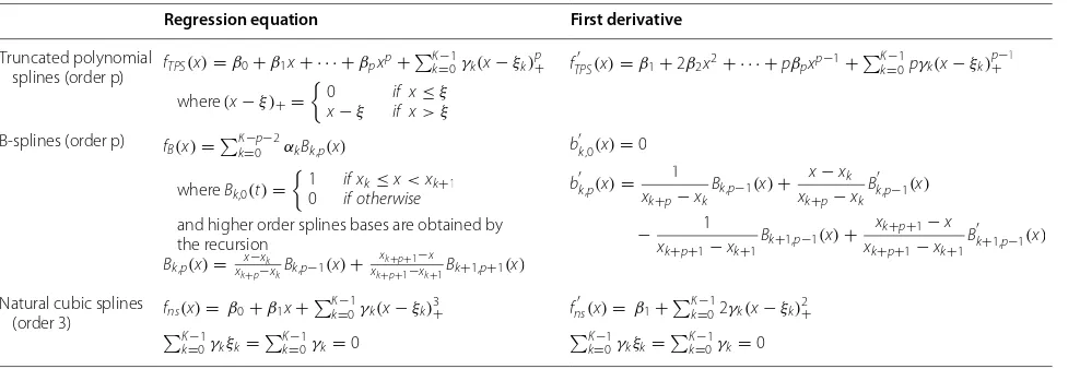
Second, we computed an estimated height velocity using the first time derivative of the longitudinal height models using standard methods (Table 1).

Biostatistical methods

The primary aim of our analysis was to model height and height velocity. We included the following predic-tors in our models: age in months, an indicator variable for greater than 24 months to account for unit differences in length vs. height measurement methods, and sex. To model the non-linear relationship between age and height over time, we used smooth, flexible functions known as cubic regression splines. While there are several forms of regression splines that can be used to model non-lin-ear relationships between a predictor (i.e., age) and an outcome (i.e., height), we chose to use cubic regression splines because they are simple to construct and under-stand [21]. We purposely varied the number and positions of the interval knots in several of our examples to demon-strate that our models are not affected by these changes. As mentioned, derivation of different types of splines to calculate height velocity is straightforward (Table 1). Since other investigators [6] have proposed the use of lin-ear splines to model child growth because of their ease of use, in this paper, we compared adequacy of both esti-mation and prediction between cubic and linear regres-sion splines with variations in the number and positions of the knots. We compared cubic and linear regression spline models using an in-sample (i.e., estimation) mean square error (MSE) and out-of-sample (i.e., prediction) MSE using standard methods. For out-of-sample predic-tion, we used 80 % of the data for training and 20 % of the data for validation. For each individual growth curve, we randomly sampled 80 % of the data values and used them to construct the model fit. The validation data consisting of 20 % of the data was then used to generate predicted height values. The predicted height and observed height were used to compute subject-specific prediction MSEs.

As described in detail below, the following statisti-cal methods were used in the model: a cubic regression spline with knots at 3, 6, 12, 18, 24 and 40 months, ran-dom intercepts and slopes to capture the heterogeneity in growth curves, and a first-order continuous autore-gressive error [CAR(1)] to capture residual serial cor-relation that arises from repeated measurements of the same child [22–24]. At each step of model building, we

∆height(tij)=

height

tij

−height(tij−1)

conducted exploratory analysis in which we visualized standardized residuals with age, a sample variogram of the residuals [25], and pairwise scatterplots of residuals at different time points to assess goodness-of-fit. We lim-ited the number of internal knots for our statistical mod-els between three and six because this number is likely sufficient to model the inflexion of linear/height growth curves in children under 5 years of age. Moreover, we also tested slight variations in the numbers and positioning of knots to determine if the model fit was affected. We con-ducted our statistical analyses in STATA 11 (StataCorp LP, College Station, TX, USA) and R ( http://www.r-pro-ject.org). Examples of statistical code in R are provided to ensure reproducibility and improve dissemination of methods (Additional file 1).

Research ethics

This study was approved by the internal review boards of A.B. PRISMA (Lima, Peru), Johns Hopkins Univer-sity (Baltimore, USA), and the European Union Ethics Committee.

Results

Baseline characteristics

We included a total of 215 children in this analysis. The initial cohort started with 304 children: however, 11 did not have available anthropometric data and 78 were lost to follow up before 1 year of age. Average follow-up was 34  months (range 12–45  months). Average number of observations per children was 50, giving a total of 10,838 observations. Of 215 children, 109 were girls (51.0 %).

Initial observations

We conducted exploratory data analysis as the first step to gain insight into the structure and nature of the data. In exploratory analysis for longitudinal data, we obtained

an understanding of the non-linear relationship of height with age but also the heterogeneity in growth curves for the study population (Fig. 1). Using a spaghetti plot of empirical height velocity, we found that it declined with age and the change was steepest at the young-est ages. In addition, in longitudinal growth data with repeated height measures, it is important to evaluate the serial autocorrelation, or the relationship between these measures. The variogram is a useful tool, as it evaluates autocorrelation by comparing the half square difference between each pair of heights within an individual to the time gap associated with each pair of heights. A nonpara-metric smooth fit is added to the variogram to describe the pattern. The exponential nonparametric smooth fit indicates that data exhibit both strong serial autocorrela-tion and heterogeneity (Fig. 1).

Building a longitudinal growth model

Our exploratory data analysis highlighted several chal-lenges that need to be addressed in modeling growth data. Specifically, we had to account for the shape of the curve, the clustering of values, the heteroge-neity among individuals, and the individual effects of serial correlation. To emphasize the role of each of these factors, we used combinations of random effects and serial correlation components in a linear model (Table 2). The steps to build the final model are described below.

Ordinary least squares model

Ordinary least squares (OLS) estimates growth param-eters by minimizing the sum of the squared vertical dis-tances between the observed and predicted responses. It provides efficient and valid predictions with the following assumptions: height can be explained by a linear com-bination of predictors, values of height are determined

Table 1 Representation of three common forms of regression splines and calculation of first derivatives

Regression equation First derivative

Truncated polynomial

splines (order p) fTPS(x)=β0+β1x+ · · · +βpx p₊K−1

k=0γk(x−ξk)p₊ where (x−ξ )₊₌

0 if x≤ξ

x−ξ if x> ξ

f_TPS′ (x)=β1+2β2x2+ · · · +pβpxp−1+Kk=−01pγk(x−ξk) p−1 +

B-splines (order p) fB(x)=K_k=−₀p−2αkBk,p(x)

where Bk,0(t)=

1 if xk≤x<xk+1 0 if otherwise

and higher order splines bases are obtained by the recursion

Bk,p(x)= xkx+−p−xkxkBk,p−1(x)+ xk+p+1−x

xk+p+1−xk+1Bk+1,p+1(x)

b′_k,0(x)=0

b′_k,p(x)= 1 xk+p−xk

Bk,p−1(x)+

x−xk xk+p−xk

B′_k,p−1(x)

− 1

xk+p+1−xk+1

Bk+1,p−1(x)+

xk+p+1−x

xk+p+1−xk+1

B′_k+1,p−1(x)

Natural cubic splines

(order 3) fns(x)= β0+β1x+

K−1

k₌0γk(x−ξk)3₊

K−1

k=0γkξk= K₋1 k=0γk=0

f_ns′(x)= β1+ K₋1

k₌02γk(x−ξk)2₊

K−1

independently of each other, height has a normal distri-bution at any particular age, and height has equal vari-ances at any particular age.

Unfortunately, growth data violates all of these assump-tions. First, growth does not follow a linear pattern with age. This can be addressed through the use cubic

Fig. 1 Panels a, c shows a spaghetti plot of the height and height velocity raw data from 50 participants respectively. Panels b, d show the

vari-ograms corresponding with each data set, where values in the x-axis represent the distance in time between two measurements and values in the y-axis (vijk) represent the square distance between those two observations [29]

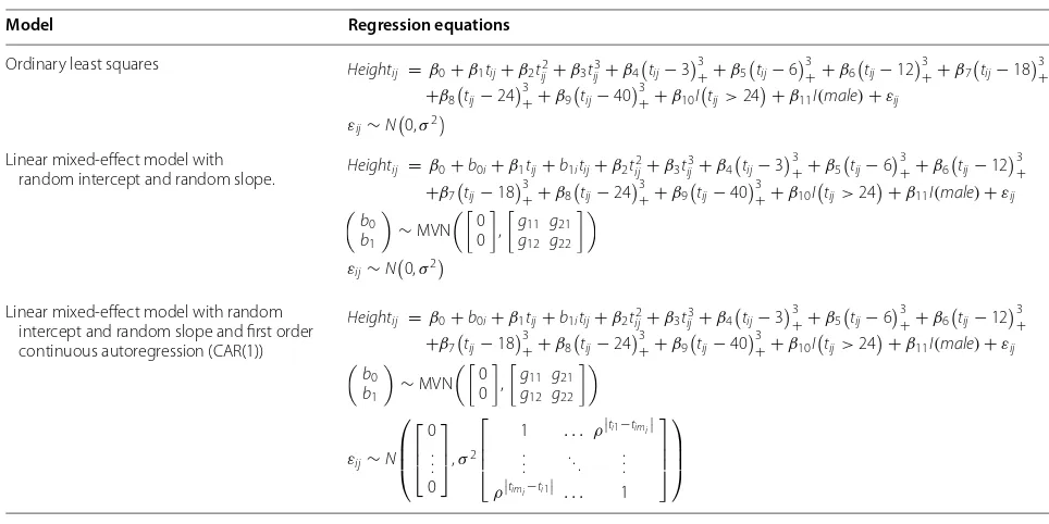
Table 2 Linear models used in our analyses

Model Regression equations

Ordinary least squares Heightij = β0+β1tij+β2t2ij+β3tij3+β4

tij−33₊+β5tij−63₊+β6tij−123₊+β7tij−183₊ +β8

tij−243₊+β9

tij−403₊+β10Itij>24+β11I(male)+εij

Linear mixed-effect model with

random intercept and random slope. Heightij = β0+b0i+β1tij+b1itij+β2t 2

ij+β3t3ij+β4

tij−33₊+β5

tij−63₊+β6

tij−123₊

+β7

tij−18 3

++β8

tij−24 3

++β9

tij−40 3

++β10I

tij>24

+β11I(male)+εij

Linear mixed-effect model with random intercept and random slope and first order continuous autoregression (CAR(1))

Heightij = β0+b0i+β1tij+b1itij+β2tij2+β3t3ij+β4

tij−33₊+β5tij−63₊+β6tij−123₊

+β7

tij−183₊+β8

tij−243₊+β9

tij−403₊+β10I

tij>24+β11I(male)+εij

εij∼N

0,σ2

b0 b1 ∼MVN 0 0 ,

g11 g21

g12 g22

εij∼N0,σ2

b0 b1 ∼MVN 0 0 ,

g11 g21

g12 g22

εij∼N        0 . . . 0   ,σ

2 

  

1 . . . ρ

� �ti1−t_imi�

� . . . . .. ... ρ � �t_imi−ti1��

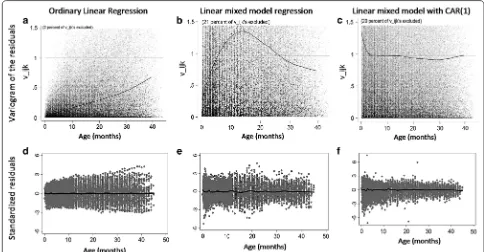
regression spline to model the curvature with age. How-ever, there are other concerns that cannot be as eas-ily adjusted by OLS. Several height measurements were taken from each child; however, these serial measure-ments of height for the same child are not independ-ent of each other. This is confirmed by a variogram of the residuals from the OLS (Fig. 2, panel a). Next, the height data did not follow a normal distribution as per the Shapiro–Wilk test (p < 0.001), the Mardia skewness test (p < 0.001), and the Mardia Kurtosis test (p < 0.001). Finally, a display of residuals versus age revealed a heter-oskedastic distribution implying that the variance of the error was not constant across ages (Fig. 2, panel d). Het-eroskedasticity was confirmed with the Breusch–Pagan test (p  <  0.001). OLS model is therefore insufficient to model longitudinal growth.

Linear mixed‑effect model without repeated measurements

The OLS model indicated that additional modeling com-ponents are necessary to account for individual-level clustering and residual autocorrelation. Linear mixed-effect models allow for non-independence and cluster-ing by describcluster-ing both between and within individual differences. We added random intercepts and slopes to the OLS model described above. Specifically, we added the parameters of the variance–covariance matrix to the

fitted model (Table 2). Our model assumes that the vari-ance–covariance of the random effects is unstructured.

At first, we only included random intercepts (b0i). The

model assumes that the random intercepts are normally distributed with mean 0 and variance g11. We found that

this parameter was statistically significant with a variance (g11) of 6.31 (95  % CI 5.21–7.62; p  <  0.001). This result

suggests that the growth of individual children diverge from the population prediction by a shift in the intercept; in other words, individual growth is shifted up or down but parallel to the population prediction.

Then, in a second step, we included both random inter-cepts and random slopes (b1i). The variance of the

inter-cept (g11) was 3.60 (95  % CI 2.97–4.36; p  <  0.001), the

range is -5.27 cm to 3.57 cm and the mean is 0.0056 cm. In addition, the variance of the slope (g22) was 0.0091 cm/

month (95  % CI 0.0075–0.011; p  <  0.001), the range is

−0.27  cm/month to 0.24  cm/month and the mean is

0.00077 cm/month (Table 3). Following the same reason-ing as for random intercepts, the random slopes repre-sent the individual variability in growth velocity around the population prediction: some individual children grow faster or slower than the population. A statistically sig-nificant variance, close to 0, as in this case, means that the shift of the individual growth velocity from the popu-lation is statistically supported but it is small. Therefore, the data exhibit less heterogeneity in the random slope

Fig. 2 Panels a, d shows the variogram and standardized residuals for the fit using OLS. Panels b, e shows for mixed model regression. Panels c, f

than in the random intercept, indicating that the main source of difference between trajectories is encapsulated in their birth height. The story could be different in other growth cohorts or on other outcomes different than growth such as blood pressure.

In our data, it was suitable to assume that the ran-dom effects follow an unstructured matrix because the random intercepts and random slopes have different variance estimates; this flexibility confers individuality to each child’s pattern of growth. The covariance (g12)

describes how the random intercept varies with the ran-dom slope. The covariance for this data set was 0.019 (95 % CI −0.0059 to 0.044; p < 0.001; Table 3). A positive covariance, as what is shown from these data, suggested that children with greater individual intercept tend to have a greater rate of growth.

The unexplained or residual variance in this model is 0.60 (95  % CI 0.59–0.62). The introduction of random effects reduced the residual variance by an order of mag-nitude from 7.34 to 0.60, implying that individual effects explain a considerable portion of the outcome variation.

To evaluate the fit of our model, we visualized stand-ardized residuals with age (Fig. 2, panel e). The linear mixed-effect model eliminated heteroskedasticity of residuals. The mixed model assumes errors are normal and conditionally independently distributed with mean zero and common variance. However, the estimated residuals did not appear randomly distributed; instead, they show symmetry in wider or narrower areas across the horizontal axis. Additionally, the variogram of the

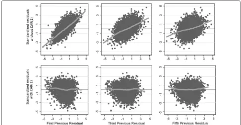
residuals still displays a degree of autocorrelation (see Fig. 2, panel b). The correlation in the residuals was con-firmed by plotting the residual versus the residual of the previous observation within a child (Fig. 3). Taken together, a mixed model was able to address the non-independence and clustering that OLS could not, and in doing so account for a greater proportion of unexplained variance and reduce the heteroskedasticity. However, it still had limitations in addressing the serial correlation from repeated measures in growth data.

Linear mixed‑effect model with CAR (1) error for repeated measurements

From the exploratory data analysis, we noted that serial height measurements within children were auto-related. We used a CAR(1) error to capture serial cor-relation in our statistical model. This structure assumes that errors are correlated and the degree of correlation is greater in those closer with age than in those further apart. The third model adds a new parameter of correla-tion ρ = 0.66 (95 % CI 0.64–0.68; p < 0.001). To evalu-ate the fit of this model, we visualized residuals with age (Fig. 2, panel f). The autocorrelation was further reduced as evidenced by the variogram of the residuals and by the lack of relationship in scatter plots of residuals ver-sus the previous observation’s residuals (Fig. 3). Both the random intercept and the random slope were statisti-cally significant and followed the same growth patterns as before (Table 3). The covariance was 0.036 (95  % CI 0.013–0.059; p  <  0.001). The unexplained variance was

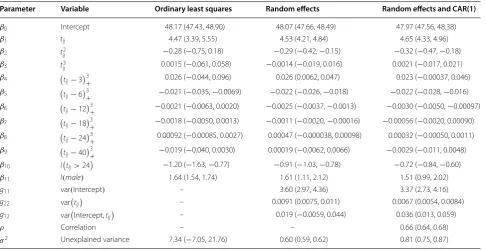
Table 3 List of estimated parameters for each individual model

Parameter Variable Ordinary least squares Random effects Random effects and CAR(1)

β0 Intercept 48.17 (47.43, 48.90) 48.07 (47.66, 48.49) 47.97 (47.56, 48.38)

β1 tij 4.47 (3.39, 5.55) 4.53 (4.21, 4.84) 4.65 (4.33, 4.96)

β2 tij2 −0.28 (−0.75, 0.18) −0.29 (−0.42, −0.15) −0.32 (−0.47, −0.18)

β3 t_ij3 0.0015 (−0.061, 0.058) −0.0014 (−0.019, 0.016) 0.0021 (−0.017, 0.021)

β4

tij−3

3

+ 0.026 (−0.044, 0.096) 0.026 (0.0062, 0.047) 0.023 (−0.00037, 0.046)

β5

tij−6

3

+ −0.021 (−0.035, −0.0069) −0.022 (−0.026, −0.018) −0.022 (−0.028, −0.016)

β6

tij−12

3

+ −0.0021 (−0.0063, 0.0020) −0.0025 (−0.0037, −0.0013) −0.0030 (−0.0050, −0.00097)

β7

tij−183₊ −0.0018 (−0.0050, 0.0013) −0.0011 (−0.0020, −0.00016) −0.00056 (−0.0020, 0.00090)

β8

tij−243₊ 0.00092 (−0.00085, 0.0027) 0.00047 (−0.000038, 0.00098) 0.00032 (−0.00050, 0.0011)

β9

tij−403₊ −0.019 (−0.040, 0.0030) 0.00019 (−0.0062, 0.0066) −0.0029 (−0.011, 0.0048)

β10 I

tij>24

−1.20 (−1.63, −0.77) −0.91 (−1.03, −0.78) −0.72 (−0.84, −0.60)

β11 I(male) 1.64 (1.54, 1.74) 1.61 (1.11, 2.12) 1.51 (0.99, 2.02)

g11 var(Intercept) – 3.60 (2.97, 4.36) 3.37 (2.73, 4.16)

g22 vartij – 0.0091 (0.0075, 0.011) 0.0067 (0.0054, 0.0084)

g12 var

Intercept,tij – 0.019 (−0.0059, 0.044) 0.036 (0.013, 0.059)

ρ Correlation – – 0.66 (0.64, 0.68)

0.81, it remained low and was similar to the unexplained variance of the linear mixed-effect model. Since there can be sex differences in child growth, we also evaluated the contribution of sex as a covariate. If all the variables remained constant, boys were on average 1.5 cm (95 % CI 0.99–2.01) taller than girls during the follow up period (Table 3).

Cubic versus linear regression splines

Cubic regression splines were superior to linear regres-sion splines in both estimation and prediction at each modeling step, and even when varying the number and position of knots. In Table 4, we report the values of AIC and BIC for OLS, LME, and LME with CAR(1) models even when the number of knots and their positions are varied. All results indicate that mixed effects models with cubic splines by far outperform the other models con-sidered and that cubic splines outperform linear splines for every level of model complexity. AIC and BIC results show that cubic splines outperform linear splines even when cubic splines use three knots and linear splines use five knots. This is probably because the growth curvature is better captured by a cubic function than by multiple piecewise linear splines. Equally importantly, however, is the important reduction in AIC and BIC noted when a CAR(1) error structure was incorporated into the regres-sion model.

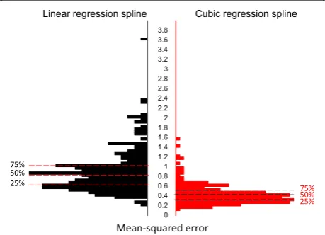
Cubic regression splines models were also better at both estimation and prediction than were linear regres-sion splines. Using three knots (at 3, 10, and 29 months) we obtained a median subject-specific estimation MSEs of 0.65 for linear regression splines and 0.51 for cubic regression splines (Fig. 4). A Kolmogorov–Smirnov test comparing the MSE distributions indicates that the two MSE distributions were different (D = 0.186, p = 0.001). Differences in the median subject-specific estima-tion MSE were similar even when the number of knots were increased, or their positions were varied (data not shown). Specifically, the out-of-sample prediction MSE was 0.86 for linear regression splines and 0.80 for cubic regression splines. These findings suggest that objective of inference in child growth problems should be primar-ily the curve and only secondarprimar-ily the coefficients.

Longitudinal models for height velocity and acceleration

With an appropriate model for height, the model for height velocity using a cubic regression spline is sim-ply obtained from its first derivative (Table 1). Similarly, growth acceleration can be obtained by taking the deriva-tive of the height velocity (formulas not shown). As a result of the derivation, the height velocity model loses the indicator variable of a difference between length and height. Also, sex is not included because our model assumes there is no interaction between sex and age. In

Fig. 3 This graph plots the standardized residuals versus the first, third and fifth previous residual. The first lane (top row) are residuals form a fit

this height velocity model, the random slope component is represented by bˆ1i.

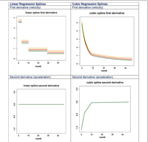
An interesting characteristic of the height velocity and acceleration curves from a cubic regression model is that they are continuous and make biological sense. In con-trast, a linear regression spline would assume that growth velocity is piecewise constant within knots but discontin-uous across knots. Moreover, growth acceleration curve is zero. Both these assumptions of linear spline approaches contradict scientific knowledge about growth trajecto-ries and the data in our application. For example, in Fig. 5

we estimated growth velocity (top panels) and accelera-tion (bottom panels) for three subjects in the study using

linear (left panels) and cubic (right panels) splines with three knots (at 3, 10, and 29 months.) A different num-ber of knots and knot locations would result in slightly different plots, but with the same qualitative interpreta-tion. The linear spline plot assumes that growth velocity is piecewise constant between the knots, an assumption that once highlighted is very difficult to accept from a sci-entific perspective. In contrast, the cubic spline estimate of the velocity curve is much more aligned with the cur-rent knowledge of human growth with the velocity curve being continuous and smooth. Even more striking, the acceleration curve estimated using linear splines is always zero. In contrast, cubic regression splines estimate a neg-ative acceleration, which is especially large in absolute terms in the first part of the curve. This corresponds to the obvious patterns we observe in growth curves: they have a slightly concave shape, with concavity much more pronounced immediately after birth (indicating decelera-tion of growth). Interestingly, the cubic spline estimator gets much closer to zero after month 10, but continues to be negative, which may indicate continuous concavity of the function, though much subtler.

Interpretation of the final model

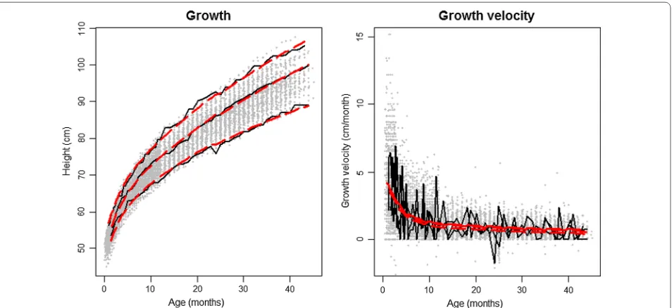
By displaying the individual growth of three children at three different percentiles and their predicted values, we can see how our model effectively reflects individual and population growth patterns (Fig. 6). Differences between children appear to be largely from shifts in intercepts, with minimal differences in growth rates. This is further supported in the height velocity model in which the three individuals have almost the same rate of growth, only dif-fering by a minimal vertical shift (Fig. 6). Therefore, the last model was able to effectively predict both population growth and differences between and within individuals in a population of Peruvian children from a peri-urban shanty town.

Table 4 Comparing the Akaike information criterion and Bayesian information criterion for linear and cubic spline mod-els using OLS (fixed effects only), LME (random slope random intercept) and LME with CAR(1) errors

Linear splines Cubic splines

Akaike information criterion

3 knots (3, 10, 29) 5 knots (3, 6, 18, 24) 3 knots (3, 10, 29) 5 knots (3, 6, 18, 24, 40)

Ordinary least squares 52,495.44 52,472.74 52,399.32 52,397.75

Random effects 28,608.28 28,345.14 27,560.38 27,541.87

Random effects and CAR(1) 19,719.72 19,495.80 19,222.76 19,235.37

Bayesian information criterion

Ordinary least squares 52,553.77 52,545.24 52,472.23 52,485.24

Random effects 28,688.47 28,439.91 27,655.15 27,651.22

Random effects and CAR(1) 19,807.21 19,597.86 19,329.66 19,352.00

0 0.2 0.4 0.6 0.81 1.2 1.4 1.6 1.8 2 2.2 2.4 2.6 2.8 3 3.2 3.4 3.6 3.8

Linear regression spline Cubic regression spline

50% 25% 75%

50% 25% 75%

Mean-squared error

Fig. 4 Subject-specific distributions of the square root MSEs for the

Discussion

The final statistical model for the prediction of height was obtained by applying a linear mixed-effect model with ran-dom intercepts and slopes, and a first-order continuous autocorrelation structure for the error term. To account for the curvature of growth with age, we used cubic regres-sion splines. To describe this modeling process, we build longitudinal growth data using a stepwise process. At each step, we examined standardized residuals with age, the

sample variogram of the residuals and pairwise scatter-plots of residuals at different time points to assess good-ness-of-fit. We also compared estimation and prediction of cubic regression spline models vis-à-vis linear regres-sion splines, and found that the former outperform the lat-ter. This suggests that inference of child growth problems should focus on differences in growth curves based on the regression parameters rather than on direct interpretation of the regression parameters themselves.

Fig. 5 Estimated growth velocity (top panels) and acceleration (bottom panels) for three subjects in the study using linear (left panels) and cubic

While a sizeable literature on modeling child growth data already exists [1–11], it should be recognized that estimation and, more importantly, prediction of subject-specific growth trajectories continues to be a problem under active methodological development and much attention needs to be given to the various choices and refinements to address the wide variety of applications. Our modeling framework adds to the literature in at least three directions. First, we are interested in fitting and predicting both at the population and subject-specific level, whereas previous related papers focus exclusively on population-level parameters [6–11]. In large studies with more than 100 children, estimating the population level parameters is relatively easy and straightforward and there is not a lot of need for modeling the subject-specific deviations. However, subject-subject-specific estima-tion and predicestima-tions is more complicated and requires a higher level of technical detail. Second, cubic regression splines provide a better fit than linear splines to non-lin-ear growth curves when the number of knots is small, as proposed by us and others. This happens because cubic regression splines capture better the non-linear trajec-tories between knots and are especially well-suited for modeling child growth immediately after birth when both acceleration and velocity are the greatest. Second, cubic regression splines assume that the velocity of growth in children is continuous and smooth whereas linear splines assume that velocity is constant in a small number of intervals, an assumption that is biologically difficult to support. Moreover, growth acceleration is a piecewise

linear and continuous function when data are modeled as cubic splines, whereas a linear spline approach assumes that growth acceleration is exactly zero. Our results indi-cate that, for this growth data set, cubic splines outper-forms linear splines when the same number and location of knots is used, and these findings are consistent with previously published work [26, 27]. In general, we rec-ommend conducting application-specific simulations to assess which model performs better. Third, modeling residuals as a continuous auto-regressive process is a fun-damentally important feature of unbalanced data that needs to be taken carefully into account.

Linear mixed-effect models are an advantageous and appropriate statistical method for longitudinal growth in children under 5 years of age. Linear mixed models not only provide information about the population predic-tion of growth but also give insight on individual patterns of growth through the random component. Our analysis also points to the importance of adequately accounting for autocorrelation of repeated measurements. Inclu-sion of cubic regresInclu-sion splines when compared to linear splines to model the curvature of growth is supported by our data because more measurements were taken when growth was faster. Also, linear mixed models allow for the analysis of unbalanced data with ease, e.g. subjects with a different number of observations and observa-tions measured at different points in time. From a meth-odological and logistical perspective, this is an advantage because sometimes it is hard to ensure that subjects do not miss any visits and that they are measured at the

Fig. 6 Observed and predicted growth for 3 individual children at different percentiles. In black are the observed growth curves and in red the

exact scheduled time. Linear mixed-effect models can account for some bias because subjects with complete follow up time might differ from subjects lost during the follow up period [28]. In addition, linear mixed-effect models support several variance–covariance matrices and structure of the residuals, allowing flexibility for vari-ous types of data with different levels of clustering, the inclusion of time-varying and time-invariant covariates and an efficient method to account for repeated measure-ments [17, 18].

A limitation of linear mixed-effect model approach presented in this paper is that not all the statistical soft-ware packages support the generation of variograms for longitudinal data, and may therefore require program-ming. Our analysis has some additional shortcomings. First, our inferences are based on the analysis of a single dataset. Second, the population under study consisted of a rather homogenous group of children with a high number of height measurements in early childhood. We acknowledge that there may be differences in statistical modeling approaches in study samples that exhibit more heterogeneity and have fewer measurements during early childhood. Third, our analytical approach requires the assumption that growth data are missing at random, in which case mixed effects models are very robust. If outcome data were not missing at random (e.g. the child was sick for a long period of time), then this can lead to larger prediction errors due to subject-specific biases. Finally, we did not include an interaction between sex and age to simplify our illustration of the statistical prin-ciples of our analysis; however, this model may not be realistic for human growth or perhaps for other longitu-dinal outcomes.

In conclusion, we present a stepwise approach to devel-oping longitudinal growth models using linear mixed-effect models that account for random mixed-effects and serial autocorrelation with cubic regression splines to capture the non-linear relationship between age and growth in height. As compared to other approaches, this mod-eling approach is simpler, direct and does not require multiple steps of transformation, analyzing age intervals separately or estimating LMS parameters. The growth velocity model obtained from the derivative eliminates measurement error directly from the growth without the need of assuming negative increments as no growth. Moreover, models based on cubic regression splines out-perform those based on linear regression splines, sug-gesting that inferences should be based on differences in growth curves based on parameters and not on the interpretation of the parameters themselves. Therefore, researchers who seek to model longitudinal child growth in their investigations would benefit from using these steps for mixed modeling in future analyses.

Abbreviations

CAR(1): continuous autoregression of order 1; OLS: ordinary least squares; TPS: truncated polynomial spline.

Authors’ contributions

LM: Developed the analytical plan, drafted the initial manuscript, and approved the final manuscript as submitted. AI: Developed and applied mixed effects model software, conducted simulations, provided results, and contrib-uted to manuscript development and responses to reviewers. MS: Coordi-nated and supervised data collection of the original study in Peru, critically reviewed the manuscript and approved the final manuscript as submitted. CC: Critically reviewed and provided input to develop the linear mixed-effect models, critically reviewed the manuscript and approved the final manu-script as submitted. DJ: Critically reviewed the manumanu-script, contributed to writing and approved the final manuscript as submitted. RHG, JC, DK, VC: Involved in study design and conduct, critically reviewed the manuscript and approved the final manuscript as submitted. LC: Coordinated and supervised data collection of the original study at the site at Peru. WC: Conceptualized and designed the original study and developed the analytical plan, critically reviewed the manuscript, and approved the final manuscript as submitted. All authors read and approved the final manuscript.

Author details

1 _{Program in Global Disease Control and Epidemiology, Department} of International Health, Bloomberg School of Public Health, Johns Hopkins University, Baltimore, USA. 2 _{Department of Mathematical Sciences, Montclair} State University, Montclair, NJ, USA. 3 _{Asociación Benéfica PRISMA, Lima, Peru.} 4 _{Departamento de Microbiología, Universidad Peruana Cayetano Heredia,} Lima, Peru. 5 _{Department of Biostatistics, Bloomberg School of Public Health,} Johns Hopkins University, Baltimore, USA. 6 _{Leeds Institute of Molecular} Medicine, St James’s University Hospital, Leeds, UK. 7 _{School of Medicine,} Trinity College Dublin and Dublin Molecular Medicine Centre, Dublin, Ireland. 8 _{Division of Parasitic Disease, Centers for Disease Control, Atlanta, USA.} 9 Divi-sion of Pulmonary and Critical Care, Department of Medicine, Johns Hopkins University, 1800 Orleans Ave Suite 9121, Baltimore, MD, USA.

Acknowledgements

This study was funded by the European Union CONTENT Framework VI project INCO-CT-2006-032136. We are grateful to the community of Pampas de San Juan de Miraflores for their long-term collaboration.

Competing interests

The authors declare that they have no competing interests.

Funding sources

Data collection was supported by the Sixth Framework Programme of the European Union, Project CONTENT (INCO-DEV-3-032136). William Checkley and Ciprian Crainiceanu were further supported by a Bill & Melinda Gates Foundation Grant (OPP1114097).

Financial disclosure statement

The authors have no financial relationships relevant to this article to disclose.

Received: 23 July 2015 Accepted: 4 December 2015

References

1. Quetelet A. Sur l’homme et le développement de ses facultés, ou Essai de physique sociale. Paris: Bachelier, imprimeur-libraire, quai des Augustins, no. 55, 1835.

Additional file

• We accept pre-submission inquiries

• Our selector tool helps you to find the most relevant journal • We provide round the clock customer support

• Convenient online submission • Thorough peer review

• Inclusion in PubMed and all major indexing services • Maximum visibility for your research

Submit your manuscript at www.biomedcentral.com/submit

Submit your next manuscript to BioMed Central

and we will help you at every step:

2. Roberts C. The Physical development and proportions of the human body. St. George’s Hosp Rep. London, vol 8, 1874–76. p 1–48. 3. Boas F. Observations on the growth of children. Science. 1930;72:44–8. 4. Falkner F, Tanner JM. Human growth: a comprehensive treatise. New York:

Plenum Press; 1986.

5. Tanner JM. A history of the study of human growth. Cambridge: Cam-bridge University Press; 1981.

6. Howe LD, Tilling K, Matijasevich A, Petherick ES, Santos AC, Fairley L, Wright J4, Santos IS, Barros AJ, Martin RM, Kramer MS, Bogdanovich N, Matush L, Barros H, Lawlor DA. Linear spline multilevel models for sum-marizing childhood growth trajectories: a guide to their application using examples from five birth cohorts. Stat Methods Med Res 2013 [Epub ahead of print].

7. Fairley L, Petherick ES, Howe LD, Tilling K, Cameron N, Lawlor DA, West J, Wright J. Describing differences in weight and length growth trajectories between white and Pakistani infants in the UK: analysis of the Born in Bradford birth cohort study using multilevel linear spline models. Arch Dis Child. 2013;98:274–9.

8. Tilling K, Davies N, Windmeijer F, Kramer MS, Bogdanovich N, Matush L, Patel R, Smith GD, Ben-Shlomo Y, Martin RM. Promotion of Breastfeeding Intervention Trial (PROBIT) study group. Is infant weight associated with childhood blood pressure? Analysis of the Promotion of Breastfeeding Intervention Trial (PROBIT) cohort. Int J Epidemiol. 2011;40:1227–37. 9. Roth DE, Perumal N, A Al Mahmud, Baqui AH. Maternal vitamin D3

supplementation during the third trimester of pregnancy: effects on infant growth in a longitudinal follow-up study in Bangladesh. J Pediatr. 2013;163:1605–11.

10. Checkley W, Epstein LD, Gilman RH, Black RE, Cabrera L, Sterling CR. Effects of Cryptosporidium parvum infection in Peruvian children: growth faltering and subsequent catch-up growth. Am J Epidemiol. 1998;148:497–506.

11. Checkley W, Epstein LD, Gilman RH, Cabrera L, Black RE. Effects of acute diarrhea on linear growth in Peruvian children. Am J Epidemiol. 2003;157:166–75.

12. Louis TA, Robins J, Dockery DW, Spiro A 3rd, Ware JH. Explaining discrep-ancies between longitudinal and cross-sectional models. J Chronic Dis. 1986;39(10):831–9.

13. Borghi E, de Onis M, Garza C, Van den Broeck J, Frongillo EA, Grummer-Strawn L, et al. Construction of the World Health Organization child growth standards: selection of methods for attained growth curves. Stat Med. 2006;25:247–65.

14. Rigby RA, Stasinopoulos DM. Generalized additive models for location, scale and shape. Applied Stat. 2005;54:507–54.

15. Rigby RA, Stasinopoulos DM. Smooth centile curves for skew and kurtotic data modelled using the Box-Cox power exponential distribution. Stat Med. 2004;23:3053–76.

16. Goldstein H. Efficient statistical modelling of longitudinal data. Ann Hum Biol. 1986;13:129–41.

17. Laird NM, Ware JH. Random-effects models for longitudinal data. Biomet-rics. 1982;38:963–74.

18. Cnaan A, Laird NM, Slasor P. Using the general linear mixed model to analyse unbalanced repeated measures and longitudinal data. Stat Med. 1997;16:2349–80.

19. Naumova EN, Must A, Laird NM. Tutorial in biostatistics: evaluating the impact of ‘critical periods’ in longitudinal studies of growth using piece-wise mixed effects models. Int J Epidemiol. 2001;30:1332–41.

20. Jaganath D, Saito M, Gilman RH, Queiroz DM, Rocha GA, Cama V, Cabrera L, Kelleher D, Windle HJ, Crabtree JE, Checkley W. First detected Helicobac-ter pylori infection in infancy modifies the association between diarrheal disease and childhood growth in Peru. Helicobacter. 2014;19:272–9. 21. Crainiceanu CM, Ruppert D, Wand MP. Bayesian analysis for penalized

spline regression using Win BUGS. J Stat Softw. 2005;14:1–24. 22. Funatogawa I, Funatogawa T, Ohashi Y. An autoregressive linear mixed

effects model for the analysis of longitudinal data which show profiles approaching asymptotes. Stat Med. 2007;26:2113–30.

23. Jones RH, Boadi-Boateng F. Unequally spaced longitudinal data with AR(1) serial correlation. Biometrics. 1991;47:161–75.

24. Ugrinowitsch C, Fellingham GW, Ricard MD. Limitations of ordinary least squares models in analyzing repeated measures data. Med Sci Sports Exerc. 2004;36:2144–8.

25. Diggle PJ. An approach to the analysis of repeated measurements. Biom-etrics. 1988;44:959–71.

26. Ruppert D, Wand MP, Carroll RJ. Semiparametric Regression. Cambridge: Cambridge University Press; 2003.

27. Wood S. Generalized additive models: an introduction with R. New York: Chapman & Hall; 2006.