Turing learning: a metric-free approach to inferring behavior and its application to swarms

DOI 10.1007/s11721-016-0126-1

Turing learning: a metric-free approach to inferring

behavior and its application to swarms

Wei Li1 _{· Melvin Gauci}2 _{·Roderich Groß}1

Received: 13 March 2016 / Accepted: 29 July 2016 / Published online: 30 August 2016 © The Author(s) 2016. This article is published with open access at Springerlink.com

Abstract We proposeTuring Learning, a novel system identification method for inferring the behavior of natural or artificial systems.Turing Learningsimultaneously optimizes two populations of computer programs, one representingmodelsof the behavior of the system under investigation, and the other representingclassifiers. By observing the behavior of the system as well as the behaviors produced by the models, two sets of data samples are obtained. The classifiers are rewarded for discriminating between these two sets, that is, for correctly categorizing data samples as either genuine or counterfeit. Conversely, the models are rewarded for ‘tricking’ the classifiers into categorizing their data samples as genuine. Unlike other methods for system identification,Turing Learningdoes not require predefined metrics to quantify the difference between the system and its models. We present two case studies with swarms of simulated robots and prove that the underlying behaviors cannot be inferred by a metric-based system identification method. By contrast,Turing Learninginfers the behaviors with high accuracy. It also produces a useful by-product—the classifiers— that can be used to detect abnormal behavior in the swarm. Moreover, we show thatTuring Learningalso successfully infers the behavior of physical robot swarms. The results show

All authors have contributed equally to this work.

Electronic supplementary material The online version of this article (doi:10.1007/s11721-016-0126-1) contains supplementary material, which is available to authorized users.

B

wei.li11@sheffield.ac.uk Melvin Gauci

mgauci@g.harvard.edu

1 _{Department of Automatic Control and Systems Engineering, The University of Sheffield, Mappin} Street, Sheffield S1 3JD, UK

that collective behaviors can be directly inferred from motion trajectories of individuals in the swarm, which may have significant implications for the study of animal collectives. Further-more,Turing Learningcould prove useful whenever a behavior is not easily characterizable using metrics, making it suitable for a wide range of applications.

Keywords System identification·Turing test·Collective behavior·Swarm robotics· Coevolution·Machine learning

1 Introduction

System identification is the process of modeling natural or artificial systems through observed data. It has drawn a large interest among researchers for decades (Ljung 2010;Billings 2013). A limitation of current system identification methods is that they rely on predefined metrics, such as the sum of square errors, to measure the difference between the output of the models and that of the system under investigation. Model optimization then proceeds by minimizing the measured differences. However, for complex systems, defining a metric can be non-trivial and case-dependent. It may require prior information about the systems. Moreover, an unsuitable metric may not distinguish well between good and bad models, or even bias the identification process. This paper overcomes these problems by introducing a system identification method that does not rely on predefined metrics.

A promising application of such a metric-free method is the identification of collective behaviors, which are emergent behaviors that arise from the interactions of numerous simple individuals (Camazine et al. 2003). Inferring collective behaviors is particularly challenging, as the individuals not only interact with the environment but also with each other. Typically, their motion appears stochastic and is hard to predict (Helbing and Johansson 2011). For instance, given a swarm of simulated fish, one would have to evaluate how close its behavior is to that of a real fish swarm, or how close the individual behavior of a simulated fish is to that of a real fish. Characterizing the behavior at the level of the swarm is difficult (Harvey et al. 2015). Such a metric may require domain-specific knowledge; moreover, it may not be able to discriminate among distinct individual behaviors that lead to similar collective dynamics (Weitz et al. 2012). Characterizing the behavior at the level of individuals is also difficult, as even the same individual fish in the swarm is likely to exhibit a different trajectory every time it is being looked at.

In this paper, we proposeTuring Learning, a novel system identification method that allows a machine to autonomously infer the behavior of a natural or artificial system.Turing Learningsimultaneously optimizes two populations of computer programs, one representing

modelsof the behavior, and the other representingclassifiers. The purpose of the models is to imitate the behavior of the system under investigation. The purpose of the classifiers is to discriminate between the behaviors produced by the system and any of the models. InTuring Learning, all behaviors are observed for a period of time. This generates two sets of data samples. The first set consists ofgenuinedata samples, which originate from the system. The second set consists ofcounterfeitdata samples, which originate from the models. The classifiers are rewarded for discriminating between samples of these two sets: Ideally, they should recognize any data sample from the system as genuine, and any data sample from the models as counterfeit. Conversely, the models are rewarded for their ability to ‘trick’ the classifiers into categorizing their data samples as genuine.

are produced as a by-product of the identification process. The method is inspired by the Turing test (Turing 1950;Saygin et al. 2000;Harnad 2000), which machines can pass if behaving indistinguishably from humans. Similarly, the models could pass the tests by the classifiers if behaving indistinguishably from the system under investigation. We hence call our methodTuring Learning.

In the following, we examine the ability ofTuring Learningto infer the behavioral rules of a swarm of mobile agents. The agents are either simulated or physical robots. They execute known behavioral rules. This allows us to compare the inferred models to the ground truth. To obtain the data samples, we record the motion trajectories of all the agents. In addition, we record the motion trajectories of an agentreplica, which is mixed into the group of agents. The replica executes the rules defined by the models—one at a time. As will be shown, by observing the motion trajectories of agents and of the agent replica,Turing Learning

automatically infers the behavioral rules of the agents. The behavioral rules examined here relate to two canonical problems in swarm robotics: self-organized aggregation (Gauci et al. 2014c) and object clustering (Gauci et al. 2014b). They are reactive; in other words, each agent maps its inputs (sensor readings) directly onto the outputs (actions). The problem of inferring the mapping is challenging, as the inputs are not known. Instead,Turing Learning

has to infer the mapping indirectly, from the observed motion trajectories of the agents and of the replica.

We originally presented the basic idea ofTuring Learning, along with preliminary simu-lations, inLi et al.(2013,2014). This paper extends our prior work as follows:

• It presents an algorithmic description ofTuring Learning;

• It shows thatTuring Learningoutperforms a metric-based system identification method in terms of model accuracy;

• It proves that the metric-based method is fundamentally flawed, as the globally optimal solution differs from the solution that should be inferred;

• It demonstrates, to the best of our knowledge for the first time, that system identification can infer the behavior of swarms of physical robots;

• It examines in detail the usefulness of the classifiers;

• It examines through simulation howTuring Learningcan simultaneously infer the agent’s brain (controller) and an aspect of its morphology that determines the agent’s field of view;

• It demonstrates through simulation thatTuring Learningcan infer the behavior even if the agent’s control system structure is unknown.

This paper is organized as follows. Section2discusses related work. Section3describes

Turing Learningand the general methodology of the two case studies. Section4investigates the ability ofTuring Learningto infer two behaviors of swarms of simulated robots. It also presents a mathematical analysis, proving that these behaviors cannot be inferred by a metric-based system identification method. Section5presents a real-world validation of Turing Learningwith a swarm of physical robots. Section6concludes the paper.

2 Related work

This section is organized as follows. First, we outline our previous work onTuring Learning

coevolutionary algorithms (but with predefined metrics), as well as work on the evolution of physical systems. Finally, works using replicas in ethological studies are presented.

Turing Learningis a system identification method that simultaneously optimizes a pop-ulation of models and a poppop-ulation of classifiers. The objective for the models is to be indistinguishable from the system under investigation. The objective for the classifiers is to distinguish between the models and the system. The idea ofTuring Learningwas first proposed inLi et al.(2013); this work presented a coevolutionary approach for inferring the behavioral rules of a single agent. The agent moved in a simulated, one-dimensional envi-ronment. Classifiers were rewarded for distinguishing between the models and the agent. In addition, they were able to control the stimulus that influenced the behavior of the agent. This allowed the classifiers to interact with the agent during the learning process.Turing Learning

was subsequently investigated with swarms of simulated robots (Li et al. 2014).

Goodfellow et al.(2014) proposedgenerative adversarial nets (GANs). GANs, while independently invented, are essentially based on the same idea asTuring Learning. The authors used GANs to train models for generating counterfeit images that resemble real images, for example, from the Toronto Face Database [for further examples, see (Radford et al. 2016)]. They simultaneously optimized a generative model (producing counterfeit images) and a discriminative model that estimates the probability of an image to be real. The optimization was done using a stochastic gradient descent method.

In a work reported inHerbert-Read et al.(2015), humans were asked to discriminate between the collective motion of real and simulated fish. The authors reported that the humans could do so even though the data from the model were consistent with the real data according to predefined metrics. Their results “highlight a limitation of fitting detailed models to real-world data.” The authors argued that “observational tests […] could be used to cross-validate models” [see alsoHarel(2005)]. This is in line withTuring Learning. Our method, however, automatically generates both the models and the classifiers, and thus does not require human observers.

metrics were critical for evaluating the performance of models. Moreover, the algorithms are not applicable to the scenarios we consider here, as the system’s inputs are assumed to be unknown (the same would typically also be the case for biological systems).

Some studies also investigated the implementation of evolution directly in physical envi-ronments, on either a single robot (Floreano and Mondada 1996;Zykov et al. 2004;Bongard et al. 2006;Koos et al. 2013;Cully et al. 2015) or multiple robots (Watson et al. 2002; O’Dowd et al. 2014;Heinerman et al. 2015). InBongard et al.(2006), a four-legged robot was built to study how it can infer its own morphology through a process of continuous self-modeling. The robot ran a coevolutionary algorithm on its onboard processor. One pop-ulation evolved models for the robot’s morphology, while the other evolved actions (inputs) to be conducted on the robot for gauging the quality of these models. Note that this approach required knowledge of the robot’s inputs (sensor data).O’Dowd et al.(2014) presented a dis-tributed approach to coevolve onboard simulators and controllers for a swarm of ten robots. Each robot used its simulators to evolve controllers for performing foraging behavior. The best performing controller was then used to control the physical robot. The foraging per-formances of the robot and of its neighbors were then compared to inform the evolution of simulators. This physical/embodied evolution helped reduce thereality gapbetween the simulated and physical environments (Jakobi et al. 1995). In all these approaches, the model optimization was based on predefined metrics (explicit or implicit).

The use of replicas can be found in ethological studies in which researchers use robots that interact with animals (Vaughan et al. 2000;Halloy et al. 2007;Faria et al. 2010;Halloy et al. 2013;Schmickl et al. 2013). Robots can be created and systematically controlled in such a way that they are accepted as conspecifics or heterospecifics by the animals in the group (Krause et al. 2011). For example, inFaria et al.(2010), a replica fish, which resembled sticklebacks in appearance, was created to investigate two types of interaction: recruitment and leadership. InHalloy et al.(2007), autonomous robots, which executed a model, were mixed into a group of cockroaches to modulate their decision making of selecting a shelter. The robots behaved in a similar way to the cockroaches. Although the robots’ appearance was different from that of the cockroaches, the robots released a specific odor such that the cockroaches would perceive them as conspecifics. In these works, the models were manually derived and the robots were only used for model validation. We believe that this robot–animal interaction framework could be enhanced throughTuring Learning, which autonomously infers the collective behavior.

3 Methodology

In this section, we present theTuring Learningmethod and show how it can be applied to two case studies in swarm robotics.

3.1 Turing learning

Algorithm 1Turing Learning

1:procedureTuring learning

2: initialize population ofMmodels and population ofNclassifiers 3: whiletermination criterion not metdo

4: for allclassifiersi∈ {1,2, . . . ,N}do

5: obtain genuine data samples (system,classifieri) 6: for each sample, obtain and store output of classifieri

7: for allmodelsj∈ {1,2, . . . ,M}do

8: obtain counterfeit data samples (modelj,classifieri) 9: for each sample, obtain and store output of classifieri

10: end for

11: end for

12: reward models (rm) for misleading classifiers (classifier outputs)

13: reward classifiers (rc) for making correct judgements (classifier outputs)

14: improve model and classifier populations based onrmandrc

15: end while 16:end procedure

Turing Learningsimultaneously optimizes two populations of computer programs, one representingmodelsof the behavior, and the other representingclassifiers. The purpose of the models is to imitate the behavior of the system under investigation. The models are used to produce data samples—we refer to these data samples ascounterfeit. There are thus two sets of data samples: one containing genuine data samples, and the other contain-ing counterfeit ones. The purpose of the classifiers is to discriminate between these two sets. Given a data sample, the classifiers need to judge where it comes from. Is it gen-uine, and thus originating from the system under investigation? Or is it counterfeit, and thus originating from a model? This setup is akin of a Turing test; hence the nameTuring Learning.

The models and classifiers are competing. The models are rewarded for ‘tricking’ the clas-sifiers into categorizing their data samples as genuine, whereas the clasclas-sifiers are rewarded for correctly categorizing data samples as either genuine or counterfeit.Turing Learningthus optimizes models for producing behaviors that are seemingly genuine, in other words, indis-tinguishablefrom the behavior of interest. This is in contrast to other system identification methods, which optimize models for producing behavior that isas similar as possibleto the behavior of interest. The Turing test inspired setup allows for model generation irrespective of whether suitable similarity metrics are known.

The model can be any computer program that can be used to produce data samples. It must however be expressive enough to produce data samples that—from an observer’s perspective—are indistinguishable from those of the system.

The classifier can be any computer program that takes a sequence of data as input and produces a binary output. The classifier must be fed with sufficient information about the behavior of the system. If it has access to only a subset of the behavioral information, any system characteristic not influencing this subset cannot be learned. In principle, classifiers with non-binary outputs (e.g., probabilities or confidence levels) could also be considered.

Algorithm1provides a description ofTuring Learning. We assume a population ofM>1 models and a population ofN >1 classifiers. After an initialization stage,Turing Learning

proceeds in an iterative manner until a termination criterion is met.

cycle.1For simplicity, we assume that each of theN classifiers is provided withK ≥1 data samples for the system and with one data sample for every model.

A model’s quality is determined by its ability of misleading classifiers to judge its data samples as genuine. Letmi j =1 if classifieriwrongly classified the data sample of model

j, andmi j=0 otherwise. The quality of modeljis then given by:

rm(j)=

1

N

N

i=1

mi j. (1)

A classifier’s quality is determined by how well it judges data samples from both the system and its models. The quality of classifieriis given by:

rc(i)=

1

2(specificityi+sensitivityi). (2)

Thespecificityof a classifier (in statistics, also called the true-negative rate) denotes the percentage of genuine data samples that it correctly identified as such. Formally,

specificity_i = 1

K

K

k=1

ai k, (3)

whereai k=1 if classifiericorrectly classified thekth data sample of the system, andai k=0

otherwise.

Thesensitivityof a classifier (in statistics, also called the true-positive rate) denotes the percentage of counterfeit data samples that it correctly identified as such. Formally,

sensitivity_i = 1

M

M

j=1

(1−mi j). (4)

Using the solution qualities,rmandrc, the model and classifier populations are improved.

In principle, any population-based optimization method can be used.

3.2 Case studies

In the following, we examine the ability ofTuring Learningto infer the behavioral rules of swarmingagents. The swarm is assumed to be homogeneous; it comprises a set of identical agents of known capabilities. The identification task thus reduces to inferring the behavior of a single agent. The agents are robots, either simulated or physical. The agents have inputs (corresponding to sensor reading values) and outputs (corresponding to motor commands). The input and output values are not known. However, the agents are observed and their motion trajectories are recorded. The trajectories are provided toTuring Learningusing a reactive control architecture (Brooks 1991). Evidence indicates that reactive behavioral rules are sufficient to produce a range of complex collective behaviors in both groups of natural and artificial agents (Braitenberg 1984;Arkin 1998;Camazine et al. 2003). Note that although reactive architectures are conceptually simple, learning their parameters is not trivial if the agent’s inputs are not available, as is the case in our problem setup. In fact, as shown in Sect.4.5, a conventional (metric-based) system identification method fails in this respect.

Fig. 1 An e-puck robot fitted with a black ‘skirt’ and a top marker for motion tracking

3.2.1 Agents

The agents move in a two-dimensional, continuous space. They are differential-wheeled robots. The speed of each wheel can be independently set to [−1,1], where −1 and 1 correspond to the wheel rotating backwards and forwards, respectively, with maximum speed. Figure1shows the agent platform, the e-puck (Mondada et al. 2009), which is used in the experiments.

Each agent is equipped with a line-of-sight sensor that detects the type of item in front of it. We assume that there arentypes [e.g., background, other agent, object (Gauci et al. 2014c,b)]. The state of the sensor is denoted byI ∈ {0,1, . . . ,n−1}.

Each agent implements a reactive behavior by mapping the input (I) onto the outputs, that is, a pair of predefined speeds for the left and right wheels,(vI, vr I),vI, vr I ∈[−1,1].

Givennsensor states, the mapping can be represented using 2nsystem parameters, which we denote as:

p=(v0, vr0, v1, vr1,· · ·, v(n−1), vr(n−1)). (5)

Usingp, any reactive behavior for the above agent can be expressed. In the following, we consider two example behaviors in detail.

Aggregation:In this behavior, the sensor is binary, that is,n=2. It gives a reading ofI=1 if there is an agent in the line of sight, andI = 0 otherwise. The environment is free of obstacles. The objective of the agents is to aggregate into a single compact cluster as fast as possible. Further details, including a validation with 40 physical e-puck robots, are reported inGauci et al.(2014c).

The aggregation controller was found by performing a grid search over the space of possible controllers (Gauci et al. 2014c). The controller exhibiting the highest performance was:

p=(−0.7,−1.0,1.0,−1.0) . (6) WhenI =0, an agent moves backwards along a clockwise circular trajectory (v0= −0.7

andvr0= −1.0). WhenI=1, an agent rotates clockwise on the spot with maximum angular

speed (v1=1.0 andvr1= −1.0). Note that, rather counterintuitively, an agent never moves

initial configuration after 60 s after 180 s after 300 s

Fig. 2 Snapshots of the aggregation behavior of 50 agents in simulation

initial configuration after 20 s after 40 s after 60 s

Fig. 3 Snapshots of the object clustering behavior in simulation. There are 5 agents (dark blue) and 10 objects (green) (Color figure online)

Object Clustering:In this behavior, the sensor is ternary, that is,n =3. It gives a reading ofI = 2 if there is an agent in the line of sight,I =1 if there is an object in the line of sight, andI =0 otherwise. The objective of the agents is to arrange the objects into a single compact cluster as fast as possible. Details of this behavior, including a validation using 5 physical e-puck robots and 20 cylindrical objects, are presented inGauci et al.(2014b).

The controller’s parameters, found using an evolutionary algorithm (Gauci et al. 2014b), are:

p=(0.5,1.0,1.0,0.5,0.1,0.5) . (7) When I = 0 andI = 2, the agent moves forward along a counterclockwise circular trajectory, but with different linear and angular speeds. WhenI=1, it moves forward along a clockwise circular trajectory. Figure3shows snapshots from a simulation trial with 5 agents and 10 objects.

3.2.2 Models and replicas

We assume the availability ofreplicas, which must have the potential to produce data samples that—to an external observer (classifier)—are indistinguishable from those of the agent. In our case, the replicas have the same morphology as the agent, including identical line-of-sight sensors and differential drive mechanisms.2

The replicas execute behavioral rules defined by the model. We adopt two model repre-sentations: gray box and black box. In both cases, note that the classifiers, which determine the quality of the models, have no knowledge about the agent/model representation or the agent/model inputs.

– In a gray box representation, the agent’s control system structure is assumed to be known. In other words, the model and the agent share the same control system structure, as defined in Eq. (5). This representation reduces the complexity of the identification process, in the sense that only the parameters of Eq. (5) need to be inferred. Additionally, this allows for an objective evaluation of how well the identification process performs, because one can compare the inferred parameters directly with the ground truth.

– In a black box representation, the agent’s control system structure is assumed to be unknown, and the model has to be represented in a general way. In particular, we use a control system structure with memory, in the form of a neural network with recurrent connections (see Sect.4.6.2).

The replicas can be mixed into a group of agents or separated from them. By default, we consider the situation that one or multiple replicas are mixed into a group of agents. The case of studying groups of agents and groups of replicas in isolation is investigated in Sect.4.6.3.

3.2.3 Classifiers

The classifiers need to discriminate between data samples originating from the agents and ones originating from the replicas. We use the termindividualto refer to either the agent or a replica executing a model.

A data sample comes from the motion trajectory of an individual observed for the duration of a trial. We assume that it is possible to track both the individual’s position and orienta-tion. The sample comprises the linear speed(s)and angular speed(ω).3_{Full details (e.g.,}

trial duration) are provided in Sects.4.2and5.3for the cases of simulation and physical experiments, respectively.

The classifier is represented as an Elman neural network (Elman 1990). The network has

i =2 inputs (sandω),h =5 hidden neurons and one output neuron. Each neuron of the hidden and output layers has a bias. The network thus has a total of(i+1)h+h2_+(h+1)=46

parameters, which all assume values inR. The activation function used in the hidden and the output neurons is the logistic sigmoid function, which has the range(0,1)and is defined as:

sig(x)= 1

1+e−x, ∀x∈R. (8)

The data sample consists of a time series, which is fed sequentially into the classifier neural network. The final value of the output neuron is used to make the judgment: model, if its value is less than 0.5, and agent otherwise. The network’s memory (hidden neurons) is reset after each judgment.

3.2.4 Optimization algorithm

The optimization of models and classifiers is realized using an evolutionary algorithm. We use a(μ+λ)evolution strategy with self-adaptive mutation strengths (Eiben and Smith 2003) to optimize either population. As a consequence, the optimization consists of two processes, one for the model population, and another for the classifier population. The two processes synchronize whenever the solution qualities described in Sect.3.1are computed. The implementation of the evolutionary algorithm is detailed inLi et al.(2013).

For the remainder of this paper, we adopt terminology used in evolutionary computing and refer to the quality of solutions as theirfitnessand to iteration cycles asgenerations. Note that in coevolutionary algorithms, each population’s fitness depends on the performance of the other populations and is hence referred to as thesubjectivefitness. By contrast, the fitness measure as used in conventional evolutionary algorithms is referred to as theobjectivefitness.

3.2.5 Termination criterion

The algorithm stops after running for a fixed number of iterations.

4 Simulation experiments

In this section, we present the simulation experiments for the two case studies. Sections4.1 and4.2, respectively, describe the simulation platform and setups. Sections4.3and4.4, respectively, analyze the inferred models and classifiers. Section4.5comparesTuring Learn-ingwith a metric-based identification method and mathematically analyzes this latter method. Section4.6presents further results of testing the generality ofTuring Learning through exploring different scenarios, which include: (i) simultaneously inferring the control of the agent and an aspect of its morphology; (ii) using artificial neural networks as a model repre-sentation, thereby removing the assumption of a known agent control system structure; (iii) separating the replicas and the agents, thereby allowing for a potentially simpler experimental setup; and (iv) inferring arbitrary reactive behaviors.

4.1 Simulation platform

We use the open-source Enki library (Magnenat et al. 2011), which models the kinematics and dynamics of rigid objects, and handles collisions. Enki has a built-in 2D model of the e-puck. The robot is represented as a disk of diameter 7.0 cm and mass 150 g. The inter-wheel distance is 5.1 cm. The speed of each wheel can be set independently. Enki induces noise on each wheel speed by multiplying the set value by a number in the range(0.95,1.05) chosen randomly with uniform distribution. The maximum speed of the e-puck is 12.8 cm/s, forwards or backwards. The linof-sight sensor is simulated by casting a ray from the e-puck’s front and checking the first item with which it intersects (if any). The range of this sensor is unlimited in simulation.

In the object clustering case study, we model objects as disks of diameter 10 cm with mass 35 g and a coefficient of static friction with the ground of 0.58, which makes it movable by a single e-puck.

The robot’s control cycle is updated every 0.1 s, and the physics is updated every 0.01 s.

4.2 Simulation setups

-1.5 -1.0 -0.5 0.0 0.5 1.0 1.5

v0 vr0 v1 vr1

model parameter

v

a

lue

of

mo

del

parameters

(a)Aggregation

-1.5 -1.0 -0.5 0.0 0.5 1.0 1.5

v0 vr0 v1 vr1 v2 vr2 model parameter

v

a

lue

o

f

m

o

del

parameters

(b) Object Clustering

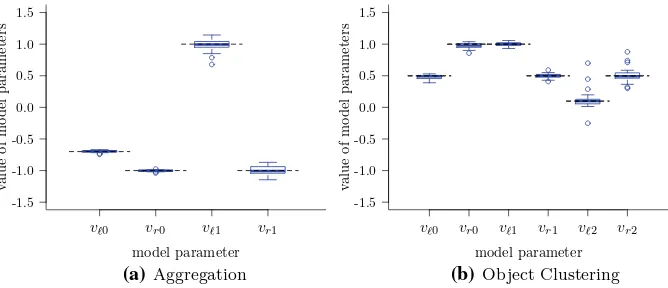
Fig. 4 Model parametersTuring Learninginferred from swarms of simulated agents performing (a) aggre-gation and (b) object clustering. Each box corresponds to the models with the highest subjective fitness in the 1000th generation of 30 runs. Thedashed black linescorrespond to the values of the parameters that the system is expected to learn (i.e., those of the agent) (Color figure online)

= 1000 cm2_{). In both case studies, individual starting orientations are chosen randomly in} [−π, π)with uniform distribution.

We performed 30 runs of Turing Learningfor each case study. Each run lasted 1000 generations. The model and classifier populations each consisted of 100 solutions (μ=50, λ=50). In each trial, classifiers observed individuals for 10 s at 0.1 s intervals (100 data points). In both setups, the total number of samples for the agents in each generation was equal tont×na, wherent is the number of trials performed (one per model) andna is the

number of agents in each trial.

4.3 Analysis of inferred models

In order to objectively measure the quality of the models obtained throughTuring Learning, we define two metrics. Given a candidate model (candidate controller)x and the agent (original controller)p, wherex ∈ R2n _{andp ∈ [−1,1]}2n_{, we define the absolute error}

(AE) in a particular parameteri ∈ {1,2, . . . ,2n}as:

AEi = |xi−pi|. (9)

We define the mean absolute error (MAE) over all parameters as:

MAE= 1

2n 2n

i=1

AEi. (10)

Figure4shows a box plot4 of the parameters of the inferred models with the highest subjective fitness value in the final generation. It can be seen thatTuring Learningidentifies the parameters for both behaviors with good accuracy (dashed black lines represent the ground truth, that is, the parameters of the observed swarming agents). In the case of aggregation, the means (standard deviations) of the AEs in the parameters are (from left to right in Fig.4a):

1 200 400 600 800 1000 -1.5 -1 -0.5 0 0.5 1 1.5 generation v a lue of mo del

parameters v0

vr0

v1

vr1

(a)Aggregation

1 200 400 600 800 1000

-1.5 -1 -0.5 0 0.5 1 1.5 generation v a lue of mo del parameters v0

vr0

v1

vr1

v2

vr2

(b) Object Clustering

Fig. 5 Evolutionary dynamics of model parameters for the (a) aggregation and (b) object clustering case studies.Curvesrepresent median parameter values of the models with the highest subjective fitness across 30 runs ofTuring Learning.Dashed black linesindicate the ground truth (Color figure online)

0.01(0.01), 0.01(0.01), 0.07(0.07), and 0.06(0.04). In the case of object clustering, these values are as follows: 0.03(0.03), 0.04(0.03), 0.02(0.02), 0.03(0.03), 0.08(0.13), and 0.08(0.09).

We also investigate the evolutionary dynamics. Figure5shows how the model parameters converge over generations. In the aggregation case study (see Fig.5a), the parameters cor-responding toI =0 are learned first. After around 50 generations, bothv0andvr0closely

approximate their true values (−0.7 and−1.0). ForI =1, it takes about 200 generations for bothv1andvr1to converge. A likely reason for this effect is that an agent spends a larger

proportion of its time seeing nothing(I=0)than seeing other agents(I=1)—simulations revealed these percentages to be 91.2 and 8.8 % respectively (mean values over 100 trials).

In the object clustering case study (see Fig.5b), the parameters corresponding toI =0 andI =1 are learned faster than the parameters corresponding toI =2. After about 200 generations,v0,vr0,v1, andvr1start to converge; however, it takes about 400 generations for

v2andvr2to approximate their true values. Note that an agent spends the highest proportion

of its time seeing nothing(I =0), followed by seeing objects(I=1)and seeing other agents (I =2)—simulations revealed these proportions to be 53.2, 34.2, and 12.6 %, respectively (mean values over 100 trials).

Although the inferred models approximate the agents well in terms of parameters, it is not uncommon in swarm systems that small changes in individual behavior lead to vastly different emergent behaviors, especially when using large numbers of agents (Levi and Kernbach 2010). For this reason, we evaluate the quality of the emergent behaviors that the models give rise to. In the case of aggregation, we measure dispersion of the swarm after some elapsed time as defined inGauci et al.(2014c).5For each of the 30 models with the highest subjective fitness in the final generation, we performed 30 trials with 50 replicas executing the model. For comparison, we also performed 30 trials using the agent [see Eq. (6)]. The set of initial configurations was the same for the replicas and the agents. Figure6a shows the dispersion of agents and replicas after 400 s. All models led to aggregation. We performed a statistical test6on the final dispersion of the individuals between the agents and replicas for

400 500 600 700 800

0 5 10 15 20 25 30

index of controller

disp

ersion

(a)Aggregation

400 500 600 700 800

0 5 10 15 20 25 30

index of controller

disp

ersion

(b)Object Clustering

Fig. 6 aDispersion of 50 simulated agents (red box) or replicas (blue boxes), executing one of the 30 inferred models in the aggregation case study.bDispersion of 50 objects when using a swarm of 25 simulated agents (red box) or replicas (blue boxes), executing one of the 30 inferred models in the object clustering case study. In both (a) and (b), boxes show the distributions obtained after 400 s over 30 trials. The models are from the 1000th generation. Thedashed black linesindicate the minimum dispersion that 50 individuals/objects can possibly achieve (Graham and Sloane 1990). See Sect.4.3for details (Color figure online)

each model. There is no statistically significant difference in 30 out of 30 cases (tests with Bonferroni correction).

In the case of object clustering, we use the dispersion of the objects after 400 s as a measure of the emergent behavior. We performed 30 trials with 25 individuals and 50 objects for the agent and each model. The results are shown in Fig.6b. In the final dispersion of objects by the agent or any of the models (replicas), there is no statistically significant difference in 26 out of 30 cases (tests with Bonferroni correction).

4.4 Analysis of generated classifiers

The primary outcome of the Turing Learningmethod (and of any system identification method) is the model, which has been discussed in the previous section. However, the gener-ated classifiers can also be considered as a useful by-product. For instance they could be used to detect abnormal agents in a swarm. We now analyze the performance of the classifiers. For the remainder of this paper, we consider only the aggregation case study.

1 6 10 60 100 600 0.5

0.6 0.7 0.8 0.9 1

generation

decision

accuracy

best classifier (subjective) best classifier (objective)

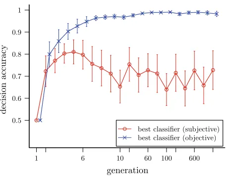
Fig. 7 Average decision accuracy of the best classifiers over 1000 generations (nonlinear scale) in 30 runs of

Turing Learning. Theerror barsshow standard deviations. See text for details

We performed 10 trials using a set of initial configurations common to all classifiers. Figure7shows the average decision accuracy of the classifier with the highest subjective fitness during the evolution (best classifier (subjective)) in 30 runs ofTuring Learning. The accuracy of the classifier increases in the first 5 generations, then drops, and fluctuates within range 62–80 %. For a comparison, we also plot the highest decision accuracy that a single classifier achieved during the post-evaluation for each generation. This classifier is referred to best classifier (objective). Interestingly, the accuracy of the best classifier (objective)

increases almost monotonically, reaching a level above 95 %. To select thebest classifier (objective), all the classifiers were post-evaluated using the aforementioned 14641 models.

At first sight, it seems counterintuitive that thebest classifier (subjective)has a low deci-sion accuracy. This phenomenon, however, can be explained when considering the model population. We have shown in the previous section (see Fig.5a) that the models converge rapidly at the beginning of the coevolutions. As a result, when classifiers are evaluated in later generations, the trials are likely to include models very similar to each other. Classifiers that become overspecialized to this small set of models (the ones dominating the later generations) have a higher chance of being selected during the evolutionary process. These classifiers may however have a low performance when evaluated across the entire model space.

Note that our analysis does not exclude the potential existence of models for which the performance of the classifiers degenerates substantially. As reported byNguyen et al.(2015), well-trained classifiers, which in their case are represented by deep neural networks, can be easily fooled. For instance, the classifiers may label a random-looking image as a guitar with high confidence. However, in this degenerate case, the image was obtained through evolutionary learning, while the classifiers remained static. By contrast, inTuring Learning, the classifiers are coevolving with the models, and hence have the opportunity to adapt to such a situation.

4.5 A metric-based system identification method: mathematical analysis and comparison withTuring Learning

observed outputs of the agents and of the models, respectively. Two outputs are considered— an individual’s linear and angular speed. Both outputs are considered over the whole duration of a trial. Formally,

em= na

i=1

T

t=1

s_m(t)−s_i(t)

2 +ω(t)

m −ω( t) i

2

, (11)

wheresm(t)ands_i(t)are the linear speed of the model and of agenti, respectively, at time step

t;ωm(t)andω(it)are the angular speed of the model and of the agenti, respectively, at time

stept;nais the number of agents in the group;Tis the total number of time steps in a trial.

4.5.1 Mathematical analysis

We begin our analysis by first analyzing an abstract version of the problem.

Theorem 1 Consider two binary random variables X and Y . Variable X takes value x1with probability p, and value x2, otherwise. Variable Y takes value y1with the same probability p, and value y2, otherwise. Variables X and Y are assumed to be independent of each other. Assuming y1and y2are given, then the metric D=E{(X−Y)2}has a global minimum at X∗with x₁∗=x₂∗=E{Y}. If p∈(0,1), the solution is unique.

Proof The probability of (i) bothx1andy1being observed is p2; (ii) bothx1andy2being

observed isp(1− p); (iii) bothx2andy1being observed is(1−p)p; (iv) bothx2andy2

being observed is(1−p)2. The expected error value,D, is then given as

D=p2(x1−y1)2+p(1−p) (x1−y2)2+(1−p)p(x2−y1)2+(1−p)2(x2−y2)2. (12)

To find the minimum expected error value, we set the partial derivatives w.r.t.x1andx2

to 0. Forx1, we have: ∂D

∂x1 =2p

2_{(x1−y1)+2p(1−p) (x1−y2)=0, (13)}

from which we obtainx₁∗=py1+(1−p)y2=E{Y}. Similarly, setting_∂∂xD2 =0, we obtain

x₂∗ = py1+(1− p)y2 = E{Y}. Note that at these values ofx1andx2, the second-order

partial derivatives are both positive [assumingp∈(0,1)]. Therefore, the (global) minimum

ofDis at this stationary point.

Corollary 1 If p∈(0,1)and y1 =y2, then X∗=Y .

Proof As p∈ (0,1), the only global minimum exists atX∗. Asx₁∗= x₂∗andy1 =y2, it

follows thatX∗=Y.

Corollary 2 Consider two discrete random variables X and Y with values x1, x2, . . . ,xn,

and y1, y2, . . . ,yn, respectively, n >1. Variable X takes value xi with probability pi and

variable Y takes value yi with the same probability pi, i =1,2, . . . ,n, where n

i=1 pi =1

and∃i,j:yi=yj. Variables X and Y are assumed to be independent of each other. Metric

D has a global minimum at X∗=Y with x₁∗=x₂∗=. . .=x_n∗=E{Y}. If all pi ∈(0,1),

Proof This proof, which is omitted here, can be obtained by examining the first and second derivatives of a generalized version of Eq. (12). Rather than four(22_{)cases, there aren}2

cases to be considered.

Corollary 3 Consider a sequence of pairs of binary random variables (Xt, Yt), t =1, . . . ,T .

Variable Xt takes value x1with probability pt, and value x2, otherwise. Variable Yt takes

value y1 with the same probability pt, and value y2 = y1, otherwise. For all t, variables Xt and Yt are assumed to be independent of each other. If all pt ∈(0,1), then the metric

D=ET_t=1(Xt−Yt)2 has one global minimum at X∗=Y .

Proof The caseT = 1 has already been considered (Theorem1and Corollary1). For the caseT =2, we extend Eq. (13) to take into accountp1andp2, and obtain

x1p2₁+p1−p2₁+p2₂+p2−p2₂=y1p₁2+p2₂+y2p1−p2₁+p2−p₂2. (14)

This can be rewritten as:

x1=

p2₁+p₂2 p1+p2

y1+

p1(1−p1)+p2(1−p2) p1+p2

y2. (15)

As y2 = y1,x1 can only be equal to y1 if p2₁+ p2₂ = p1 + p2, which is equivalent to

p1(1− p1)+ p2(1− p2) = 0. This is however not possible for any p1,p2 ∈ (0,1). Therefore,X∗=Y.7

For the general case,T ≥1, the following equation can be obtained (proof omitted).

x1=

T t=1 p2t

_T

t=1pt

y1+

T

t=1pt(1−pt)

_T

t=1pt

y2. (16)

The same argument applies—x∗₁cannot be equal toy1. Therefore,X∗=Y.

Implications for our scenario:The metric-based approach considered in this paper is unable to infer the correct behavior of the agent. In particular, the model that is globally optimal w.r.t. the expected value for the error function defined by Eq. (11) is different from the agent. This observation follows from Corollary1for the aggregation case study (two sensor states), and from Corollary2for the object clustering case study (three sensor states). It exploits the fact that the error function is of the same structure as the metric in Corollary3— a sum of square error terms. The summation over time is not of concern—as was shown in Corollary3, the distributions of sensor reading values (inputs) of the agent and of the model do not need to be stationary. However, we need to assume that for any control cycle, the actual inputs of agents and models are not correlated with each other. Note that the sum in Eq. (11) comprises two square error terms: one for the linear speed of the agent, and the other for the angular speed. As our simulated agents employ a differential drive with unconstrained motor speeds, the linear and angular speeds are decoupled. In other words, the linear and angular speeds can be chosen independently of each other, and optimized separately. This means that Eq. (11) can be thought of as two separate error functions: one pertaining to the linear speeds, and the other to the angular speeds.

7_{Note that in the case ofp}

-1.5 -1.0 -0.5 0.0 0.5 1.0 1.5

v0 vr0 v1 vr1

model parameter

v

a

lue

of

mo

del

parameters

(a)Aggregation

-1.5 -1.0 -0.5 0.0 0.5 1.0 1.5

v0 vr0 v1 vr1 v2 vr2 model parameter

v

a

lue

of

mo

del

parameters

(b)Object Clustering

Fig. 8 Model parameters a metric-based evolutionary method inferred from swarms of simulated agents performing (a) aggregation and (b) object clustering. Each box corresponds to the models with the highest fitness in the 1000th generation of 30 runs. Thedashed black linescorrespond to the values of the parameters that the system is expected to learn (i.e., those of the agent) (Color figure online)

4.5.2 Comparison with Turing Learning

To verify whether the theoretical result (and its assumptions) holds in practice, we used an evolutionary algorithm with a single population of models. The algorithm was identical to the model optimization sub-algorithm inTuring Learningexcept for the fitness calculation, where the metric of Eq. (11) was employed. We performed 30 evolutionary runs for each case study. Each evolutionary run lasted 1000 generations. The simulation setup and number of fitness evaluations for the models were kept the same as inTuring Learning.

Figure8a shows the parameter distribution of the evolved models with highest fitness in the last generation over 30 runs. The distributions of the evolved parameters corresponding toI=

0 andI=1 are similar. This phenomenon can be explained as follows. In the identification problem that we consider, the method has no knowledge of the input, that is, whether the agent perceives another agent(I =1)or not(I =0). This is consistent withTuring Learning

as the classifiers that are used to optimize the models also do not have any knowledge of the inputs. The metric-based algorithm seems to construct controllers that do not respond differently to either input, but work as good as it gets on average, that is, for the particular distribution of inputs, 0 and 1. For the left wheel speed, both parameters are approximately −0.54. This is almost identical to the weighted mean(−0.7∗0.912+1.0∗0.088= −0.5504), which takes into account that parameterv0= −0.7 is observed around 91.2 % of the time,

whereas parameterv1 = 1 is observed around 8.8 % of the time (see also Sect.4.3). The

parameters related toI =1 evolved well as the agent’s parameters are identical regardless of the input(vr0=vr1= −1.0). For bothI =0 andI =1, the evolved parameters show good

agreement with Theorem 1. As the model and the agents are only observed for 10 s in the simulation trials, the probabilities of seeing a 0 or a 1 are nearly constant throughout the trial. Hence, this scenario approximates very well the conditions of Theorem1, and the effects of non-stationary probabilities on the optimal point (Corollary3) are minimal. Similar results were found when inferring the object clustering behavior (see Fig.8b).

4.6 Generality ofTuring Learning

In the following, we present four orthogonal studies testing the generality ofTuring Learning. The experimental setup in each section is identical to that described previously (see Sect.4.2), except for the modifications discussed within each section.

4.6.1 Simultaneously inferring control and morphology

In the previous sections, we assumed that we fully knew the agents’ morphology, and only their behavior (controller) was to be identified. We now present a variation where one aspect of the morphology is also unknown. The replica, in addition to the four controller parameters, takes a parameterθ ∈[0,2π] rad, which determines the horizontal field of view of its sensor, as shown in Fig.9(the sensor is still binary). Note that the agents’ line-of-sight sensors of the previous sections can be considered as sensors with a field of view of 0 rad.

The models now have five parameters. As before, we let Turing Learningrun in an unbounded search space (i.e., now,R5). However, asθ is necessarily bounded, before a model is executed on a replica, the parameter corresponding toθ is mapped to the range (0,2π)using an appropriately scaled logistic sigmoid function. The controller parameters are directly passed to the replica. In this setup, the classifiers observe the individuals for 100 s in each trial (preliminary results indicated that this setup required a longer observation time). Figure10a shows the parameters of the subjectively best models in the last (1000th) generations of 30 runs. The means (standard deviations) of the AEs in each model parameter

(a) (b)

Fig. 9 A diagram showing the angle of view of the agent’s sensor investigated in Sect.4.6.1

-2 -1 0 1 2 3

v0 vr0 v1 vr1 θ model parameter

v

a

lue

o

f

m

o

del

parameters

(a)

-2 -1 0 1 2 3

v0 vr0 v1 vr1 θ model parameter

v

a

lue

o

f

m

o

del

parameters

(b)

are as follows: 0.02 (0.01), 0.02 (0.02), 0.05 (0.07), 0.06 (0.06), and 0.01 (0.01). All parameters includingθare still learned with high accuracy.

The case where the true value ofθ is 0 rad is an edge case, because given an arbitrarily small >0, the logistic sigmoid function maps an unbounded domain of values onto(0, ). This makes it simpler forTuring Learningto infer this parameter. For this reason, we also consider another scenario where the agents’ angle of view isπ/3 rad rather than 0 rad. The controller parameters for achieving aggregation in this case are different from those in Eq. (6). They were found by rerunning a grid search with the modified sensor. Figure10b shows the results from 30 runs with this setup. The means (standard deviations) of the AEs in each parameter are as follows: 0.04(0.04), 0.03(0.03), 0.05(0.06), 0.05(0.05), and 0.20(0.19). The controller parameters are still learned with good accuracy. The accuracy in the angle of view is noticeably lower, but still reasonable.

4.6.2 Inferring behavior without assuming a known control system structure

In the previous sections, we assumed the agent’s control system structure to be known and only inferred its parameters. To further investigate the generality ofTuring Learning, we now rep-resent the model in a more general form, namely a (recurrent) Elman neural network (Elman 1990). The network inputs and outputs are identical to those used for our reactive models. In other words, the Elman network has one input(I)and two outputs representing the left and right wheel speed of the robot. A bias is connected to the input and hidden layers of the network, respectively. We consider three network structures with one, three, and five hidden neurons, which correspond, respectively, to 7, 23, and 47 weights to be optimized. Except for a different number of parameters to be optimized, the experimental setup is equivalent in all aspects to that of Sect.4.2.

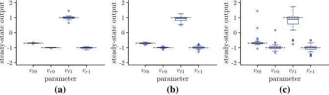
We first analyze the steady-state behavior of the inferred network models. To obtain their steady-state outputs, we fed them with a constant input (I = 0 or I = 1 depending on the parameters) for 20 time steps. Figure11shows the outputs in the final time step of the inferred models with the highest subjective fitness in the last generation in 30 runs for the three cases. In all cases, the parameters of the swarming agent can be inferred correctly with reasonable accuracy. More hidden neurons lead to worse results, probably due to the larger search space.

We now analyze the dynamic behavior of the inferred network models. Figure12shows the dynamic output of 1 of the 30 neural networks. The chosen neural network is the one

-2 -1 0 1 2

v0 vr0 v1 vr1

parameter stea dy-s ta te output

(a)

-2 -1 0 1 2

v0 vr0 v1 vr1

parameter stea dy-s ta te out pu t (b) -2 -1 0 1 2

v0 vr0 v1 vr1

parameter stea dy-s tate ou tpu t (c)

1 5 9 13 17 21 25 29 -2 -1 0 1 2 time step d ynamic output

I= 0 I= 1 I= 0

o or

(a)

1 5 9 13 17 21 25 29

-2 -1 0 1 2 time step d ynam ico u tput

I= 0 I= 1 I= 0

o or

(b)

1 5 9 13 17 21 25 29

-2 -1 0 1 2 time step dynamic ou tput

I= 0 I= 1 I= 0

o or

(c)

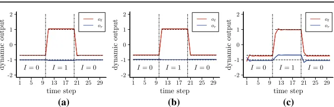
Fig. 12 Dynamic outputs of the inferred neural network with median performance. The network’s input in each case wasI=0 (time steps 1–10),I=1 (time steps 11–20), andI=0 (time steps 21–30). See text for details.aOne hidden neuron,bThree hidden neurons,cFive hidden neurons

exhibiting the median performance according to metric4_i=120_t=1(oi t −pi)2, where pi

denotes theith parameter in Eq. (6), andoi tdenotes the output of the neural network in the

tth time step corresponding to theith parameter in Eq. (6). The inferred networks react to the inputs rapidly and maintain a steady-state output (with little disturbance). The results show thatTuring Learningcan infer the behavior without assuming the agent’s control system structure to be known.

4.6.3 Separating the replicas and the agents

In our two case studies, the replica was mixed into a group of agents. In the context of animal behavior studies, a robot replica may be introduced into a group of animals and recognized as a conspecific (Halloy et al. 2007;Faria et al. 2010). However, if behaving abnormally, the replica may disrupt the behavior of the swarm (Bjerknes and Winfield 2013). For the same reason, the insertion of a replica that exhibits different behavior or is not recognized as conspecific may disrupt the behavior of the swarm and hence the models obtained may be biased. In this case, an alternative method would be to isolate the influence of the replica(s). We performed an additional simulation study where agents and replicas were never mixed. Instead, each trial focused on either a group of agents, or of replicas. All replicas in a trial executed the same model. The group size was identical in both cases. The tracking data of the agents and the replicas from each sample were then fed into the classifiers for making judgments.

The distribution of the inferred model parameters is shown in Fig.13. The results show thatTuring Learningcan still identify the model parameters well. There is no significant difference between either approach in the case studies considered in this paper. The method of separating replicas and agents is recommended if potential biases are suspected.

4.6.4 Inferring other reactive behaviors

The aggregation controller that agents used in our case study was originally synthesized by searching over the parameter space defined in Eq. (5) withn=2, using a metric to assess the swarm’s global performance (Gauci et al. 2014c). Each of these points produces a global behavior. Some of these behaviors are particularly interesting, such as the circle formation behavior reported inGauci et al.(2014a).

Fig. 13 Model parameters inferred by a variant ofTuring Learningthat observes swarms of aggregating agents and swarms of replicas in isolation, thereby avoiding potential bias. Each box corresponds to the models with the highest subjective fitness in the 1000th generation of 30 simulation runs

-1.5 -1.0 -0.5 0.0 0.5 1.0 1.5

v0 vr0 v1 vr1

model parameter

v

alue

o

f

m

o

del

parameters

MAE

frequency

0.00 0.02 0.04 0.06 0.08 0.10

0 100 200 300 400

(

a

)

0.0 0.5 1.0 1.5 2.0

v0 vr0 v1 vr1

model parameter

AE

(b)

Fig. 14 Turing Learninginferring the models for 1000 randomly generated agent behaviors. For each behavior, one run ofTuring Learningwas performed and the model with the highest subjective fitness after 1000 generations was considered.aHistogram of the models’ MAE [(defined in Eq. (10); 43 points that have an MAE larger than 0.1 are not shown]; andbAEs [defined in Eq. (9)] for each model parameter

in the parameter space defined in Eq. (5), with uniform distribution. For each controller, we performed one run, and selected the subjectively best model in the last (1000th) generation. Figure14a shows a histogram of the MAE of the inferred models. The distribution has a single mode close to zero and decays rapidly for increasing values. Over 89 % of the 1000 cases have an error below 0.05. This suggests that the accuracy ofTuring Learning

is not highly sensitive to the particular behavior under investigation (i.e., most behaviors are learned equally well). Figure14b shows the AEs of each model parameter. The means (standard deviations) of the AEs in each parameter are as follows: 0.01(0.05), 0.02(0.07), 0.07(0.6), and 0.05(0.2). We performed a statistical test on the AEs between the model parameters corresponding toI =0 (v0andvr0) andI =1 (v1 andvr1). The AEs of the

inferredv0andvr0 are significantly lower than those ofv1andvr1. This is likely due to

Replica

Agents _{Overhead Camera}

Computer

video stream (robot positions & orientations)

model updates

Robot Arena

start/stop signal

Fig. 15 Illustration of the general setup for inferring the behavior of physical agents—e-puck robots (not to scale). The computer runs theTuring Learningalgorithm, which produces models and classifiers. The models are uploaded and executed on the replica. The classifiers run on the computer. They are provided with the agents’ and replica’s motion data, extracted from the video stream of the overhead camera

5 Physical experiments

In this section, we present a real-world validation ofTuring Learning. We explain how it can be used to infer the behavior of a swarm of real agents. The agents and replicas are represented by physical robots. We use the same type of robot (e-puck) as in simulation. The agents execute the aggregation behavior described in Sect.3.2.1. The replicas execute the candidate models. We use two replicas to speed up the identification process, as will be explained in Sect.5.3.

5.1 Physical platform

The physical setup, shown in Fig.15, consists of an arena with robots (representing agents or replicas), a personal computer (PC), and an overhead camera. The PC runs theTuring Learningalgorithm. It communicates with the replicas, providing them models to be executed, but does not exert any control over the agents. The overhead camera supplies the PC with a video stream of the swarm. The PC performs video processing to obtain motion data about individual robots. We now describe the physical platform in more detail.

5.1.1 Robot arena

The robot arena is rectangular with sides 200 cm×225 cm and bounded by walls of 50 cm high. The floor has a light gray color, and the walls are painted white.

5.1.2 Robot platform and sensor implementations

Fig. 16 Schematic top view of an e-puck, indicating the locations of its motors, wheels, camera, and infrared sensors. Note that the marker is pointing toward the robot’s back

orientation. The gray values from these pixels are used to distinguish robots(I =1)against the arena(I =0). For more details about this sensor realization, see (Gauci et al. 2014c).

We also use the e-puck’s infrared sensors, in two cases. Firstly, before each trial, the robots disperse themselves within the arena. In this case, they use the infrared sensors to avoid both robots and walls, making the dispersion process more efficient. Secondly, we observe that using only the line-of-sight sensor can lead to robots becoming stuck against the walls of the arena, hindering the identification process. We therefore use the infrared sensors for wall avoidance, but in such a way as to not affect inter-robot interactions.8Details of these two collision avoidance behaviors are provided in the online supplementary materials (Li et al. 2016).

5.1.3 Motion capture

To facilitate motion data extraction, we fit robots with markers on their tops, consisting of a colored isosceles triangle on a circular white background (see Fig.1). The triangle’s color allows for distinction between robots; we use blue triangles for all agents, and orange and purple triangles for the two replicas. The triangle’s shape eases extraction of robots’ orientations.

The robots’ motion is captured using a camera mounted around 270 cm above the arena floor. The camera’s frame rate is set to 10 fps. The video stream is fed to the PC, which performs video processing to extract motion data about individual robots (position and ori-entation). The video processing software is written using OpenCV (Bradski and Kaehler 2008).

5.2Turing Learningwith physical robots

Our objective is to infer the agent’s aggregation behavior. We do not wish to infer the agent’s dispersion behavior, which is periodically executed to distribute already-aggregated agents. To separate these two behaviors, the robots (agents and replicas) and the system are implicitly synchronized. This is realized by making each robot execute a fixed behavioral loop of

Fig. 17 Flow diagram of the programs run by the PC and a replica in the physical experiments.Dashed arrows

represent communication between the two units. See Sect.5.2for details. The PC does not exert any control over the agents

constant duration. The PC also executes a fixed behavioral loop, but the timing is determined by the signals received from the replicas. Therefore, the PC is synchronized with the swarm. The PC communicates with the replicas via Bluetooth. At the start of a run, or after a human intervention (see Sect.5.3), robots are initially synchronized using an infrared signal from a remote control.

Figure17shows a flow diagram of the programs run by the PC and the replicas, respec-tively. Dashed arrows indicate communication between the units.

The program running on the PC has the following states:

• P1. Wait for “Stop” Signal.The program is paused until “Stop” signals are received from both replicas. These signals indicate that a trial has finished.

• P2. Send Model Parameters.The PC sends new model parameters to the buffer of each replica.

• P3. Wait for “Start” Signal.The program is paused until “Start” signals are received from both replicas, indicating that a trial is starting.

• P4. Track Robots.The PC waits 1 s and then tracks the robots using the overhead camera for 5 s. The tracking data contain the positions and orientations of the agents and replicas. • P5. Update Turing Learning Algorithm. The PC uses the motion data from the trial observed inP4to update the solution quality (fitness values) of the corresponding two models and all classifiers. Once all models in the current iteration cycle (generation) have been evaluated, the PC also generates new model and classifier populations. The method for calculating the qualities of solutions and the optimization algorithm are described in Sects.3.1and3.2.4, respectively. The PC then goes back toP1.

The program running on the replicas has the following states:

• R1. Send “Stop” Signal. After a trial stops, the replica informs the PC by sending a “Stop” signal. The replica waits 1 s before proceeding withR2, so that all robots remain synchronized. Waiting 1 s in other states serves the same purpose.