Development of a new pan-European testate amoeba transfer function
for reconstructing peatland palaeohydrology
Matthew J. Amesbury
a,*, Graeme T. Swindles
b, Anatoly Bobrov
c, Dan J. Charman
a,
Joseph Holden
b, Mariusz Lamentowicz
d, Gunnar Mallon
e, Yuri Mazei
f,g,
Edward A.D. Mitchell
h, Richard J. Payne
f,i, Thomas P. Roland
a, T. Edward Turner
b,
Barry G. Warner
jaGeography, College of Life and Environmental Sciences, University of Exeter, UK bWater@leeds, School of Geography, University of Leeds, UK
cFaculty of Soil Science, Lomonosov Moscow State University, Russia
dLaboratory of Wetland Ecology and Monitoring&Department of Biogeography and Palaeoecology, Faculty of Geographical and Geological Sciences, Adam Mickiewicz University, Poland
eDepartment of Geography, University of Sheffield, UK
fDepartment of Zoology and Ecology, Penza State University, Russia gDepartment of Hydrobiology, Lomonosov Moscow State University, Russia hInstitute of Biology, Faculty of Science, University of Neuch^atel, Switzerland iEnvironment, University of York, UK
jEarth and Environmental Sciences, University of Waterloo, Canada
a r t i c l e i n f o
Article history:
Received 22 July 2016 Received in revised form 22 September 2016 Accepted 23 September 2016 Available online 13 October 2016
Keywords:
Testate amoeba Peatland Water table Transfer function Europe Spatial scale Data compilation Taxonomy
a b s t r a c t
In the decade since thefirst pan-European testate amoeba-based transfer function for peatland palae-ohydrological reconstruction was published, a vast amount of additional data collection has been un-dertaken by the research community. Here, we expand the pan-European dataset from 128 to 1799 samples, spanning 35 of latitude and 55 of longitude. After the development of a new taxonomic scheme to permit compilation of data from a wide range of contributors and the removal of samples with high pH values, we developed ecological transfer functions using a range of model types and a dataset of ~1300 samples. We rigorously tested the efficacy of these models using both statistical validation and independent test sets with associated instrumental data. Model performance measured by statistical indicators was comparable to other published models. Comparison to test sets showed that taxonomic resolution did not impair model performance and that the new pan-European model can therefore be used as an effective tool for palaeohydrological reconstruction. Our results question the efficacy of relying on statistical validation of transfer functions alone and support a multi-faceted approach to the assessment of new models. We substantiated recent advice that model outputs should be standardised and presented as residual values in order to focus interpretation on secure directional shifts, avoiding potentially inaccurate conclusions relating to specific water-table depths. The extent and diversity of the dataset highlighted that, at the taxonomic resolution applied, a majority of taxa had broad geographic distributions, though some morphotypes appeared to have restricted ranges.
©2016 The Authors. Published by Elsevier Ltd. This is an open access article under the CC BY license (http://creativecommons.org/licenses/by/4.0/).
1. Introduction
Testate amoebae are microscopic, unicellular shelled protozoa that are abundant in a range of wetlands, including peatlands
(Mitchell et al., 2008). Early research demonstrated the close ecological coupling between testate amoebae and hydrological parameters such as water-table depth and moisture content in such environments (e.g. Jung, 1936; Schonborn, 1963€ ). Quantitative ecological approaches demonstrated the strength of this relation-ship and used it to derive reconstructions of hydrological variability from fossil testate amoebae (Warner and Charman, 1994; Woodland et al., 1998). This approach has subsequently been *Corresponding author.
E-mail address:[email protected](M.J. Amesbury).
Contents lists available atScienceDirect
Quaternary Science Reviews
j o u r n a l h o m e p a g e : w w w . e l s e v i e r. c o m / lo c a t e / q u a s c i r e v
http://dx.doi.org/10.1016/j.quascirev.2016.09.024
thoroughly developed and extended geographically, using more advanced statistical techniques (e.g.Charman et al., 2007; Booth, 2008; Swindles et al., 2009, 2014, 2015a; Amesbury et al., 2013). Testate amoeba-based hydrological reconstructions are now frequently used as hydroclimate proxies in studies of Holocene climate change (e.g.Charman et al., 2006; Swindles et al., 2010; Elliott et al., 2012; Lamentowicz et al., 2015; Willis et al., 2015). Central to such research is typically the application of a transfer function. These statistical models apply the observed modern ecological preferences of amoebae via a range of mathematical approaches (Juggins and Birks, 2011) to fossil assemblages to quantitatively reconstruct environmental variables of interest, primarily water-table depth in ombrotrophic peatlands, but occa-sionally other parameters such as pH (Markel et al., 2010; Mitchell et al., 2013). Testate amoeba-based hydrological transfer functions have now been developed in a wide range of locations (e.g.Li et al., 2015; Swindles et al., 2015a, 2014; van Bellen et al., 2014) and wetland types, primarily in bogs, but also in fens (Payne, 2011; Lamentowicz et al., 2013a, 2013b). Recent debates in this field have focussed on 1) more rigorous analysis of transfer function results, whether via statistical testing (Telford and Birks, 2005, 2009, 2011a, 2011b, Payne et al., 2012, 2016; Amesbury et al., 2013), or by comparison with instrumental data (Swindles et al., 2015b); 2) the appropriateness of varying spatial scales for trans-fer function development (Turner et al., 2013); and 3) the validity of applying models outside of the geographic range over which they were developed (Turner et al., 2013; Willis et al., 2015), and hence the cosmopolitanism of testate amoeba ecological preferences (Booth and Zygmunt, 2005) across a range of geographical locations (Smith et al., 2008).
When transfer function models developed in one region are applied in a different region where no local model exists, results may theoretically be undermined by a number of factors. These include missing modern analogues, differences in testate amoeba ecology or biogeography between the two regions (Turner et al., 2013), the technique used to measure water-table depth in the calibration data sets (Markel et al., 2010; e.g. long-term mean versus one-off measurement), regionally diverse seasonal vari-ability (Sullivan and Booth, 2011; Marcisz et al., 2014) or vertical zonation (van Bellen et al., 2014) of testate assemblages, or local-scale variability in the response of certain taxa, or even commu-nities, of testate amoebae to environmental variables (e.g.Booth and Zygmunt, 2005). However, in practice, when transfer func-tions from one region are applied to fossil data from a separate region, even over distances of thousands of kilometres (Turner et al., 2013; Willis et al., 2015), or when regional- and continental-scale models are compared (e.g.Amesbury et al., 2008; Charman et al., 2007; Swindles et al., 2009; Turner et al., 2013), it is largely only the absolute values and magnitude of reconstructed water-table shifts that vary between models, with the timing and direction of change being generally consistent. Given that the ab-solute values and magnitude of transfer function-reconstructed change in water-table depth have recently been questioned by direct comparison of reconstructed and instrumental water-table depths (Swindles et al., 2015b), it could be argued that a) testate amoeba-based transfer function reconstructions should be viewed as semi-quantitative and interpretation should be based only on the timing and direction of change; and that b) the general ecological cosmopolitanism of testate amoebae (e.g.Mitchell et al., 2000; Booth and Zygmunt, 2005) when studied at coarse taxo-nomic level (i.e. morphotypesebut seeHeger et al., 2013for an example of cryptic diversity showing geographical patterns) means that regional transfer functions are widely applicable, at least at an intra-continental or even intra-hemispheric scale.
Approaching a decade after the publication of thefirst testate
amoeba-based pan-European transfer function (Charman et al., 2007), which included 128 samples from seven countries, we present a new collaborative effort to vastly extend that dataset, including both published and unpublished data that increases the number of samples to 1799, from a much expanded geographical range covering 18 countries spaced over 35of latitude and 55of longitude. In doing so, we develop a new transfer function for peatland testate amoeba palaeohydrological reconstruction and shed new light on the biogeography and cosmopolitanism of testate amoebae and the potential effects of varying spatial scales and supra-regional application on resulting transfer function re-constructions. We rigorously test our newly developed models using a novel combination of statistical validation and checks against independent testate amoeba data with associated instru-mental water-table depth measurements. Ultimately, we aim to facilitate more reliable comparisons of spatial and temporal pat-terns of peatland-derived palaeoclimate records at a continental scale.
2. Methods
2.1. Data compilation and taxonomy
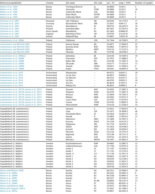
We compiled a full dataset containing 1799 samples from 113 sites in 18 countries from 31 published studies, with contributions of unpublished data from two countries (Table 1;Fig. 1). All samples in the dataset had an associated water-table depth value, whereas a reduced number (n¼1564) also had an associated pH value.
Although the potential risks of taxonomic inconsistency, espe-cially in large data compilations with large numbers of analysts, are clear (Payne et al., 2011), the likely effect of using a low taxonomic resolution is potentially decreased model performance (in statis-tical terms) rather than any effect on the timing or direction of major changes in wetness (Mitchell et al., 2014). Due to the high number of data contributors/analysts in this compilation and in order to ensure taxonomic consistency across the merged dataset, we adopted a low-resolution approach to defining an appropriate taxonomic scheme, merging morphologically similar taxa together into a series of newly defined groups. Initial examination of contributed datasets made it clear that different analysts had grouped (or‘lumped’) or split taxa to varying extents, with many taxa only present in individual datasets. A low-resolution approach to taxonomy was therefore considered to be not only the most parsimonious, but also the only scientifically valid approach to the compilation of such a large dataset, despite genuine variation in water-table optima occurring between taxa within some new groupings (see Results). As a result, individual analysts should not count new samples in line with the low-resolution taxonomic scheme applied here, but rather differentiate between readily identifiable taxa in line with current taxonomies and group taxa together only for statistical analysis. The majority of recently pub-lished papers on peatland testate amoebae use Charman et al. (2000) as a standard identification guide, with an increasing number of variations noted in recent years including, most preva-lently, the reclassification ofAmphitremaflavumasArcherellafl a-vum(Loeblich and Tappan, 1961), the splitting out of certain‘type’ groupings into their constituent taxa (e.g. Cyclopyxis arcelloides type intoCyclopyxis arcelloides sensu stricto,Phryganella acropodia and Difflugia globulosa; Turner et al., 2013) and more recent reclassifications based on phylogenetic studies (e.g. Nebela taxa moving to the genera Longinebela, Planocarinaand Gibbocarina;
Kosakyan et al., 2016).
Table 1
Site details and meta-data. Only one lat/long position was available for thefive sites in Russia ofBobrov et al. (1999)and the four sites in Greece ofPayne and Mitchell (2007). Data ordered by author surname/year and sub-divided by country/publication.
Reference/unpublished Country Site name Site code Lat (N) Long (E/W) Number of samples
Bobrov et al., 1999 Russia Tverskaya Reserve Q 56.4666 33.05 E 5
Bobrov et al., 1999 Russia Staroselia STAR 56.4666 33.05 E 10
Bobrov et al., 1999 Russia Gulnovsky Moch GUL 56.4666 33.05 E 6
Bobrov et al., 1999 Russia Katin Moch KATIN 56.4666 33.05 E 7
Bobrov et al., 1999 Russia Goltovsky Moch GOLT 56.4666 33.05 E 2
Charman et al., 2007 Denmark Lille Vildmose DK 56.8526 10.1735 E 17
Charman et al., 2007 Germany Bissendorfer Moor DM 52.5037 9.6811 E 18
Charman et al., 2007 Estonia Mannikjarve ES 58.8752 26.2479 E 18
Charman et al., 2007 Finland Kontolanrahka FI 60.7837 22.7874 E 24
Charman et al., 2007 Faroe Islands Masaklettar FO 62.1665 6.9000 W 17
Charman et al., 2007 England Butterburn Flow GB 55.0759 2.5124 W 18
Charman et al., 2007 Ireland Ballyduff Bog IR 53.0807 7.9925 W 16
Lamentowicz et al., 2008a Poland Chlebowo CHL 52.7364 16.7569 E 27
Lamentowicz and Mitchell 2005 Poland Jelenia Wyspa JEL 53.6077 17.9560 E 23
Lamentowicz and Mitchell 2005 Poland Jeziorka Kozie KOZ 53.6965 17.8974 E 10
Lamentowicz and Mitchell 2005 Poland Mietlica MIET 53.8110 17.5153 E 12
Lamentowicz and Mitchell 2005 Poland Okoniny OK 53.6740 18.0766 E 3
Lamentowicz et al., 2008a,b Poland Jedwabna JB 52.6144 19.1039 E 10
Lamentowicz et al., 2008b Poland Ostrowite OST 53.7932 17.5880 E 7
Lamentowicz et al., 2008b Poland Rybie Oko RO 53.8140 17.5387 E 19
Lamentowicz et al., 2008b Poland Skrzynka SKR 53.8171 17.5233 E 12
Lamentowicz et al., 2008b Poland Stawek STAW 53.8913 17.5566 E 9
Lamentowicz et al., 2008b Poland Sta˛zki_ STAZ 54.4241 18.0854 E 10
Lamentowicz et al., 2010 Switzerland Mauntschas e 46.4575 9.8561 E 39
Lamentowicz et al., 2010 Switzerland Lej da Staz e 46.4972 9.8694 E 11
Lamentowicz et al., 2010 Switzerland Lej Marsch e 46.4753 9.8197 E 12
Lamentowicz et al., 2010 Switzerland Lej Nair e 46.4703 9.8201 E 10
Lamentowicz et al., 2010 Switzerland Inn Fen e 46.4078 9.7027 E 13
Lamentowicz et al., 2010 Switzerland Maloja Fen e 46.4053 9.6900 E 8
Lamentowicz et al., 2013b; Jassey et al., 2014 Poland Kazanie KAZ 52.4581 17.2981 E 19
Lamentowicz et al., 2013b; Jassey et al., 2014 Poland Wagowo WAG 52.4195 17.3647 E 20
Lamentowicz et al., 2013b; Jassey et al., 2014 Poland Rurzyca RUR 53.2864 16.7203 E 23
Lamentowicz et al., 2013b; Jassey et al., 2014 Poland Maka˛ty MAK 52.6562 15.8721 E 7
Lamentowicz et al., 2013b; Jassey et al., 2014 Poland Czarci Staw CZS 53.3797 17.0759 E 15
Lamentowicz et al., 2013b; Jassey et al., 2014 Poland Czarne CZAR 52.4742 17.8893 E 18
Lamentowicz et al., 2013b; Jassey et al., 2014 Poland Wierzchołek WEK 53.4154 17.2358 E 14
Unpublished (M. Lamentowicz) Poland Zamarte Z 53.5915 17.9670 E 8 Unpublished (M. Lamentowicz) Poland Linje LIN 53.1875 18.3096 E 46 Unpublished (M. Lamentowicz) Poland Słowinskie Błoto SL 54.3624 16.4815 E 25 Unpublished (M. Lamentowicz) Poland Kuznik K 53.6965 17.8974 E 31 Unpublished (M. Lamentowicz) Poland Okoniowe OKO 53.1884 16.7997 E 5 Unpublished (M. Lamentowicz) Poland Kaczory KACZ 53.1230 16.9155 E 5 Unpublished (M. Lamentowicz) Poland Zelgniowo ZEL 53.1719 16.8701 E 5 Unpublished (M. Lamentowicz) Poland Skorki SKO 53.1852 16.9108 E 7 Unpublished (M. Lamentowicz) Poland Jeziorki JEZ 53.1458 16.8594 E 3 Unpublished (M. Lamentowicz) Poland Olszowy OLSZ 53.2126 16.7275 E 4 Unpublished (M. Lamentowicz) Poland Bagienny BAG 53.2140 16.7311 E 4 Unpublished (M. Lamentowicz) Poland Ga˛zwa GAZ 53.8732 21.2232 E 14 Unpublished (M. Lamentowicz) Poland Mechacz MECH 54.3307 22.4422 E 14 Unpublished (G. Mallon) Sweden Kortlandamossen KOR 59.8483 12.2867 E 15 Unpublished (G. Mallon) Sweden Gallseredsmossen GAL 57.1750 12.5975 E 15 Unpublished (G. Mallon) Sweden South 3 S3 57.1747 12.6342 E 15 Unpublished (G. Mallon) Sweden South 7 S7 57.1725 12.7125 E 15 Unpublished (G. Mallon) Sweden South 11 S11 57.1139 12.7811 E 15 Unpublished (G. Mallon) Sweden North 1 N1 59.8625 12.3247 E 15 Unpublished (G. Mallon) Sweden North 2 N2 59.9239 12.2728 E 15 Unpublished (G. Mallon) Sweden North 3 N3 59.8542 12.3031 E 15 Unpublished (G. Mallon) Sweden North 4 N4 59.8753 12.2914 E 15 Unpublished (G. Mallon) Sweden North 5 N5 59.8728 12.3053 E 15
Mazei and Bubnova 2009 Russia Karelia K4 66.5251 32.9386 E 10
Mazei et al., 2009a Russia Karelia K3 66.5225 32.9491 E 9
Mazei et al., 2009b Russia Karelia K2 66.5238 32.9097 E 14
Mazei et al., 2009c Russia Karelia K1 66.5227 32.9185 E 15
Mazei et al., 2009d Russia Borok B1 B4 58.0845 38.2147 E 13
Mazei et al., 2009e Russia Penza P1 52.9325 46.5031 E 5
Mazei and Bubnova 2008 Russia Penza P2 52.9575 45.5382 E 5
Mazei and Tsyganov 2007a Russia Penza P3 53.3037 45.1366 E 6
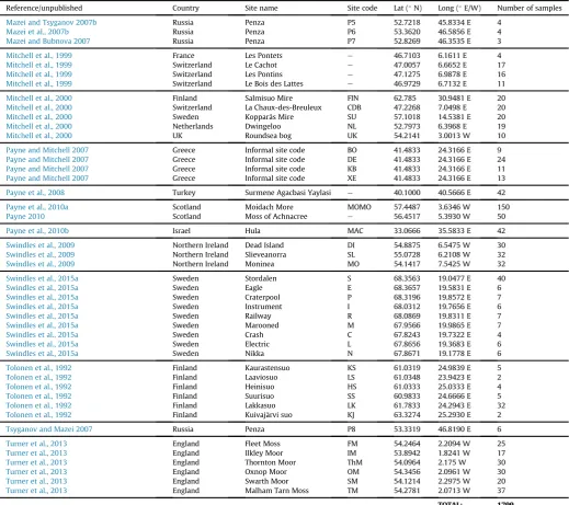
(38 newly defined) that each contained between two and 11 taxa with similar morphological features (Table 2). These groups were defined with reference to a range of identification keys and source literature (Cash and Hopkinson, 1905, 1909, Cash et al., 1915, 1918; Ogden and Hedley, 1980; Meisterfeld, 2000a, 2000b) as well as using the expertise and experience of the authors. Our treatment of the twoEuglyphagroupseE. ciliatatype andE. rotundatypee
provides an example of the low resolution approach we adopted. These groups contained 11 and eight individual taxa respectively that had been identified by individual analysts in the originally contributed datasets. However, the only morphological charac-teristic that we could identify as consistently applied across all datasets was size, with several datasets only defining E. tuberculata(i.e. larger type>45
m
m) andE. rotunda(i.e. smaller type<45m
m). Since the presence/absence of spines (e.g.E. strigosavs.E. tuberculata) may be biased by taphonomic processes (Payne et al., 2011), we therefore defaulted to a two-taxon system for this family.
[image:4.595.43.563.76.537.2]When all data were compiled using this new taxonomy, taxa which occurred in<18 samples (i.e. 1% of the data) were excluded as rare taxa (n¼8;Table 3), resulting in a total of 52 taxa in the ‘edited’dataset. With the exception ofCyphoderiasp.,Placocistasp. andTrigonopyxissp., which were included inCyphoderia ampulla type,Placocista spinosatype andTrigonopyxis arculatype respec-tively (groupings which contained all potential examples of these genera), all individuals defined only to the family level were also excluded from the dataset. Where this process resulted in a total assemblage<90% of the original total count, we excluded whole samples from the full dataset (n¼24,Table 4), resulting in a total of 1775 samples in an ‘edited’ dataset (Fig. 2). Transfer function Table 1(continued)
Reference/unpublished Country Site name Site code Lat (N) Long (E/W) Number of samples
Mazei and Tsyganov 2007b Russia Penza P5 52.7218 45.8334 E 4
Mazei et al., 2007b Russia Penza P6 53.3620 46.5856 E 4
Mazei and Bubnova 2007 Russia Penza P7 52.8269 46.3535 E 3
Mitchell et al., 1999 France Les Pontets e 46.7103 6.1611 E 4
Mitchell et al., 1999 Switzerland Le Cachot e 47.0057 6.6652 E 17
Mitchell et al., 1999 Switzerland Les Pontins e 47.1275 6.9878 E 16
Mitchell et al., 1999 Switzerland Le Bois des Lattes e 46.9729 6.7132 E 11
Mitchell et al., 2000 Finland Salmisuo Mire FIN 62.785 30.9481 E 20
Mitchell et al., 2000 Switzerland La Chaux-des-Breuleux CDB 47.2268 7.0498 E 20
Mitchell et al., 2000 Sweden Kopparås Mire SU 57.1018 14.5381 E 20
Mitchell et al., 2000 Netherlands Dwingeloo NL 52.7973 6.3968 E 19
Mitchell et al., 2000 UK Roundsea bog UK 54.2141 3.0013 W 10
Payne and Mitchell 2007 Greece Informal site code BO 41.4833 24.3166 E 9
Payne and Mitchell 2007 Greece Informal site code DE 41.4833 24.3166 E 24
Payne and Mitchell 2007 Greece Informal site code KB 41.4833 24.3166 E 11
Payne and Mitchell 2007 Greece Informal site code XE 41.4833 24.3166 E 13
Payne et al., 2008 Turkey Surmene Agacbasi Yaylasi e 40.1000 40.5666 E 42
Payne et al., 2010a Scotland Moidach More MOMO 57.4487 3.6346 W 150
Payne 2010 Scotland Moss of Achnacree e 56.4517 5.3930 W 50
Payne et al., 2010b Israel Hula MAC 33.0666 35.5833 E 42
Swindles et al., 2009 Northern Ireland Dead Island DI 54.8875 6.5475 W 30
Swindles et al., 2009 Northern Ireland Slieveanorra SL 55.0728 6.2108 W 32
Swindles et al., 2009 Northern Ireland Moninea MO 54.1417 7.5425 W 32
Swindles et al., 2015a Sweden Stordalen S 68.3563 19.0477 E 40
Swindles et al., 2015a Sweden Eagle E 68.3657 19.5831 E 6
Swindles et al., 2015a Sweden Craterpool P 68.3196 19.8572 E 7
Swindles et al., 2015a Sweden Instrument I 68.0312 19.7656 E 6
Swindles et al., 2015a Sweden Railway R 68.0869 19.8311 E 7
Swindles et al., 2015a Sweden Marooned M 67.9566 19.9865 E 7
Swindles et al., 2015a Sweden Crash C 67.8243 19.7322 E 4
Swindles et al., 2015a Sweden Electric L 67.8656 19.3683 E 6
Swindles et al., 2015a Sweden Nikka N 67.8671 19.1778 E 6
Tolonen et al., 1992 Finland Kaurastensuo KS 61.0319 24.9839 E 5
Tolonen et al., 1992 Finland Laaviosuo LS 61.0348 23.9423 E 2
Tolonen et al., 1992 Finland Heinisuo HS 61.0333 25.0333 E 4
Tolonen et al., 1992 Finland Suurisuo SS 60.9833 24.6666 E 5
Tolonen et al., 1992 Finland Lakkasuo LK 61.7833 24.2943 E 32
Tolonen et al., 1992 Finland Kuivaj€arvi suo KJ 63.3274 25.2930 E 2
Tsyganov and Mazei 2007 Russia Penza P8 53.3319 46.8190 E 6
Turner et al., 2013 England Fleet Moss FM 54.2464 2.2094 W 25
Turner et al., 2013 England Ilkley Moor IM 53.8942 1.8241 W 17
Turner et al., 2013 England Thornton Moor ThM 54.0964 2.175 W 30
Turner et al., 2013 England Oxnop Moor OM 54.3456 2.0961 W 30
Turner et al., 2013 England Swarth Moor SM 54.1214 2.2975 W 20
Turner et al., 2013 England Malham Tarn Moss TM 54.2781 2.0713 W 37
TOTAL: 1799
development proceeded from this‘edited’dataset. Hereafter, this ‘edited’dataset will be referred to as the full dataset.
2.2. Statistics
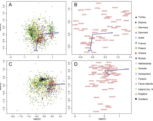
Since the full dataset contained samples from a range of different peatland types on a continuum between more oligotro-phic bogs to more eutrooligotro-phic fens (range in pH values of 2.5e8.1), and in light of the overarching aim of this study to produce a transfer function for palaeohydrological reconstruction, we initially used exploratory ordination analyses (non-metric multidimen-sional scaling (NMDS) using the Bray-Curtis dissimilarity) to objectively reduce the dataset to those samples more representa-tive of the nutrient poor, ombrotrophic peatlands commonly used in palaeoclimate research. We applied a high pH cut-off based on NMDS axis one scores and k-means cluster analysis (for additional details see ordination results). All analyses were carried out in R version 3.2.2 (R Core Team, 2015) using the packages vegan (Oksanen et al., 2015) for NMDS and cluster analysis and pvclust for significance testing between clusters (Suzuki and Shimodaira, 2014).
Transfer function development was also carried out in R (R Core Team, 2015) using the package rioja (Juggins, 2015), applying four
commonly used model types, namely: weighted averaging (WA; with and without tolerance downweighting (WA-Tol)), weighted average partial least squares (WAPLS), maximum likelihood (ML) and the modern analogue technique (MAT). In each case, only re-sults of the best performing (judged by root mean square error of prediction (RMSEP) and R2) model within each type are shown. RMSEP values were calculated using the standard leave-one-out (RMSEPLOO) technique, as well as leave-one-site-out (RMSEPLOSO; Payne et al., 2012) and segment-wise (RMSEPSW;Telford and Birks, 2011b) approaches. Spatial autocorrelation tests were calculated in the R package palaeoSig (Telford, 2015) using the ‘rne’(random, neighbour, environment) function.
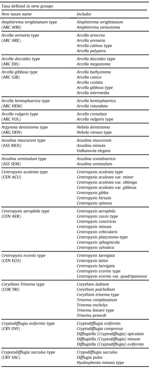
[image:5.595.87.503.65.445.2]Table 2
Summary of taxonomic scheme developed for and applied in this study, resulting in 41‘type’groupings (38 newly defined) and 19 individual taxa. Taxon codes are included.
Taxa defined in new groups
New taxon name Includes
Amphitrema wrightianumtype (ARC WRI)
Amphitrema wrightianum Amphitrema stenostoma
Arcella arenariatype (ARC ARE)
Arcella artocrea Arcella arenaria Arcella catinustype
Arcella polypora
Arcella discoidestype (ARC DIS)
Arcella discoidestype
Arcella megastoma
Arcella gibbosatype (ARC GIB)
Arcella bathystoma Arcella conica Arcella costata Arcella gibbosatype
Arcella intermedia
Arcella hemisphaericatype (ARC HEM)
Arcella hemisphaerica Arcella rotundata
Arcella vulgaristype (ARC VUL)
Arcella crenulata Arcella vulgaristype
Argynnia dentistomatype (ARG DEN)
Nebela dentistoma Nebela vitraeatype
Assulina muscorumtype (ASS MUS)
Assulina muscorum Assulina minuta Valkanovia elegans
Assulina seminulumtype (ASS SEM)
Assulina scandinavica Assulina seminulum
Centropyxis aculeatatype (CEN ACU)
Centropyxis aculeatatype
Centropyxis aculeatavar.minor Centropyxis aculeatavar.oblonga Centropyxis aculeatavar.gibbosa Centropyxis gibba
Centropyxis hirsuta Centropyxis spinosa
Centropyxis aerophilatype (CEN AER)
Centropyxis aerophila Centropyxis cassistype
Centropyxis constricta Centropyxis minuta Centropyxis orbicularis Centropyxis platystomatype
Centropyxis sphagnicola Centropyxis sylvatica
Centropyxis ecornistype (CEN ECO)
Centropyxis laevigata Centropyxis latior Centropyxis laevigata Centropyxis ecornistype
Centropyxis ecornisvar.quadripannosa Corythion-Trinematype (COR TRI) Corythion dubium Corythion pulchellum Corythion-trinematype Trinema complanatum Trinema enchelys Trinema linearetype
Trinema penardi
Cryptodifflugia oviformistype (CRY OVI)
Cryptodifflugia oviformis Cryptodifflugia compressa
Difflugiella (Cryptodifflugia) apiculata Difflugiella (Cryptodifflugia) minuta Difflugiella (Cryptodifflugia) oviformis
Crypotodifflugia sacculustype (CRY SAC)
Crypodifflugia sacculus Difflugia pulex
Hyalosphenia minutatype
Cyclopyxis arcelloidestype (CYC ARC)
Centropyxis eurystoma Cyclopyxis arcelloidestype
Cyclopyxis eurystoma Cyclopyxis kahli Difflugia globulosatype
Difflugia microstoma Phryganella acropodia Phryganella hemispherica Phryganella nidulus Phryganella paradoxa
Cyphoderia ampullatype (CYP AMP)
Cyphoderia ampulla Cyphoderia calceolus Cyphoderiasp.
Difflugia acuminatatype (DIF ACU)
Difflugia acuminatatype
Difflugia bacilliariumtype
Difflugia elegans
Difflugia gramentype (DIF GRA)
Difflugia gramen Difflugia brevicolla
Difflugia labiosatype (DIF LAB)
Difflugia amphora Difflugia oviformis/labiosa Netzelia tuberculata
Difflugia lucidatype (DIF LUC)
Difflugia avellana Difflguia glans Difflugia lithophila Difflugia lucidatype
Difflugia mica Difflugia penardi Difflugia prististype
Difflugia viscidula Pseudodifflugia fascicularis Pseudodifflugia fulvatype
Difflugia oblongatype (DIF OBL)
Difflugia bacilliferatype
Difflugia gassowski/longicollis Difflugia lacustris
Difflugia lanceolata Difflugia oblongatype
Difflugia parva Difflugia paulii Difflugia pyriformis Difflugia rubescens
Euglypha ciliatatype (EUG CIL)
Euglypha acanthophora Euglypha ciliata
Euglypha ciliatavar.glabra Euglypha ciliata/compressa Euglypha compressatype
Euglypha cristata Euglypha dolioformis Euglyphafilifera Euglypha scutigera Euglypha strigosatype
Euglypha tuberculatatype
Euglypha rotundatype (EUG ROT) Euglypha alveolata Euglypha anadonta Euglypha cuspidata Euglypha denticulata Euglypha hyalina Euglypha laevis Euglypha rotundatype
Euglypha simplex
Heleopera petricolatype (HEL PET)
Awerintzewia cyclostoma Heleopera petricola Heleopera sphagni
Heleopera petricolavaramethystea Heleopera picta
Lesqueresia spiralistype (LES SPI)
Lesquereusia modestatype
Lesquereusia spiralistype
Planocarina (Nebela) carinatatype (PLA CAR)
multiple daily measurements (for full details see source publica-tions). Sample-specific errors for the transfer function re-constructions were based on 1000 bootstrapping cycles. We compared our reconstructions with output from the previous Eu-ropean transfer function (Charman et al., 2007) and tested the significance of the new reconstructions using the ‘randomTF’ function in palaeoSig (Telford, 2015).
We used the programme PAST (version 3.10; Hammer et al., 2001) to run one-way PERMANOVA tests (9999 iterations) of the differences between samples from different countries and three assigned eco-regions (Atlantic, n ¼ 461; Scandinavia, n ¼341; Continental, n ¼500; Fig. 1) that represented broadly different climate zones and degrees of oceanicity/continentality.
3. Results
3.1. Ordination
[image:7.595.31.287.82.433.2]NMDS of the full dataset (n¼1775;Fig. 3A and B) showed that the primary environmental variable explaining species distribution along axis 1 was pH, as opposed to water-table depth, illustrating the influence of the peatland type gradient (i.e. ombrotrophic to minerotrophic). A distinct group of samples formed an outlying cluster with high NMDS axis 1 scores. To determine an appropriate pH cut-off to reduce the dataset to those containing nutrient poor, ombrotrophic peatlands, we used results of k-means cluster anal-ysis, forcing the data into two clusters (Fig. S1; i.e. lower pH values in Group 1, higher pH values in Group 2). 5.4 was the highest pH where the majority of samples fell in Group 1 and 5.5 was the lowest pH where the majority of samples fell in Group 2. We therefore removed all samples with pH5.5. This division was supported by plotting NMDS scores against pH, which showed an Table 3
Taxa occurring in<18 samples (<1% of the full dataset) excluded from the full dataset, resulting in an edited dataset of 52 taxa.
Taxon code n Full name
ARC MIT 2 Arcella mitrata
CAM MIN 11 Campascus minutus
DIF URC 12 Difflugia urceolatatype LAG VAS 8 Lagenodifflugia vas
LES EPI 14 Lesquereusia epistomum
PLAGIO 8 Plagiopyxistype
PON ELI 1 Pontigulasia elisa
[image:7.595.302.553.94.181.2]PSE GRA 3 Pseudodifflugia gracilis
Table 4
Samples with total %s<90 when‘sp.’taxa were deleted which were excluded from the full dataset, resulting in an edited dataset of 1775 samples.
Country Site name Code % Removed Sweden Gallseredsmossen GAL_3 14.3
Sweden South S11_8 11.0
Poland Chlebowo CHL1 19.6
Poland Chlebowo CHL7 27.4
Poland Chlebowo CHL22 31.2 Poland Chlebowo CHL23 40.9
Poland Kuznik K07 10.3
Poland Kuznik K09 10.9
Poland Kuznik K14 13.0
Poland Rurzyca RUR23 23.1
Poland Wierzchołek WEK2 28.2 Poland Wierzchołek WEK5 19.6 Poland Wierzchołek WEK6 40.4 Poland Wierzchołek WEK11 40.2 Poland Wierzchołek WEK12 12.8 Poland Wierzchołek WEK13 19.3 Poland Wierzchołek WEK14 46.2 Russia Tverskya Reserve Q92_1 11.4 Russia Staroselia STAR_1 19.0 Russia Katin Moch KATIN_5 10.3 Russia Katin Moch KATIN_6 44.4 Russia Katin Moch KATIN_7 19.3 England Thornton Moor TM85 14.5
[image:7.595.303.553.229.455.2]Sweden Crash C1 17.6
Table 2(continued)
Taxa defined in new groups
New taxon name Includes
Nebela collaristype (NEB COL)
Nebela collaristype
Nebela tinctavar.major Hyalosphenia ovalis
Gibbocarina (Nebela) penardianatype (GIB PEN)
Gibbocarina (Nebela) penardianatype
Gibbocarina (Nebela) gracilis Gibbocarina (Nebela) tubulosatype
Nebela tinctatype (NEB TIN)
Nebela tincta Nebela parvula Nebela bohemicatype
Padaungiella lageniformistype (PAD LAG)
Nebela lageniformis Nebela wailesitype
Nebela tubulata
Physochila griseolatype Nebela griseolatype (PHY GRI) Nebela tenella Placocista spinosatype
(PLA SPI)
Placocista spinosatype
Placocista lens Placocista gracilis Placocista jurassica Placocistasp.
Plagiopyxistype (PLAGIO)
Plagiopyxis callida Plagiopyxis declivis
Pyxidicula operculatatype (PYX OPE)
Pyxidicula declivis Pyxidicula operculata
Sphenoderiatype (SPHENO)
Sphenoderiafissirostris Sphenoderia lenta Sphenoderia lenta/fissirostris
Tracheleuglypha dentatatype (TRA DEN)
Tracheleuglypha dentata Tracheleuglypha acolla
Trigonopyxis arculatype (TRI ARC)
Trigonopyxis arculatype
Trigonopyxis minutatype
Trigonopyxissp. Individual taxa/types not redefined
Arcella dentata(ARC DEN)
Arcella mitrata(ARC MIT)
Archerellaflavum(ARC FLA)
Bullinularia indica(BUL IND)
Campascus minutus(CAM MIN)
Difflugia leidyi(DIF LEI)
Difflugia urceolatatype (DIF URC)
Heleopera rosea(HEL ROS)
Heleopera sylvatica(HEL SYL)
Hyalosphenia elegans(HEL ELE)
Hyalosphenia papilio(HYA PAP)
Hyalosphenia subflava(HYA SUB)
Lagenodifflugia vas(LAG VAS)
Lesquereusia epistomum(LES EPI)
Longinebela (Nebela) militaristype (NEB MIL)
Microclamys patella(MIC PAT)
Nebelaflabellulum(NEB FLA)
Nebela minortype (NEB MIN)
Paraquadrula irregularis(PAR IRR)
Pontigulasia elisa(PON ELI)
Pseudodifflugia gracilis(PSE GRA)
Fig. 2.Percentage distribution of all taxa. Taxa are ordered from‘wet’on the left to‘dry’on the right based on the taxa optima from the WA-Tol (inv) model of the full dataset (n¼1775).
M.J.
Amesbury
et
al.
/
Quaternary
Science
Reviews
15
2
(20
16
)
132
e
151
13
abrupt jump to higher axis 1 values at this point in the pH range (Fig. S1) and also by general peatland ecology:Sphagnummoss, the dominant peat-forming species in Northern Hemisphere ombro-trophic peatlands is known to actively acidify its environment (van Breemen, 1995) and therefore ombrotrophic bogs are typically dominated by pH ranges of 3.0e4.5, with Sphagnum-dominated poor fens having marginally higher pH (4.5e5.5;Lamentowicz and Mitchell, 2005). Using this cut-off resulted in the removal of 370 samples with pH values 5.5e8.1 and the removal of all samples from France, Greece and Israel. We re-ran NMDS ordination on the reduced, low-pH dataset (n¼1405, including samples without a pH measurement (n¼211);Fig. 3C and D) which then showed that water-table depth was the primary environmental variable explaining species variation along axis 1 (p < 0.001 using the ‘envfit’ function in vegan), providing a statistical foundation to proceed with transfer function development. Despite water-table depth being the primary explanatory variable after removal of high pH samples, there is still considerable variability along NMDS axis two (Fig. 3D) that reflects previous axis one variability (Fig. 3B), potentially driven by samples without pH values that may in reality be from sites with pH5.5. In particular, a group of nine taxa
[image:9.595.38.545.63.465.2]3.2. Transfer function development and statistical assessment
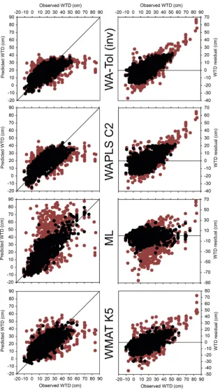
Before proceeding with transfer function development, we removed 12 further samples with extreme measured water table values (Table S1), resulting in a dataset for transfer function development of 1393 samples. These 12 samples fell below the 0.5th (i.e. representing deep surface ponding, n¼2) and above the 99.5th (i.e. representing extreme deep water tables, n¼10) per-centiles of water-table depth and were removed to avoid the large increase in water-table depth range that would result from their inclusion and the subsequent effect on removal of samples with high residual values. In addition, the removal of extreme deep water-table depth samples is supported bySwindles et al. (2015b), who showed a disconnect between testate amoebae and water table in such circumstances. In keeping with standard practice, we then ran two iterations of models, thefirst using all samples and the second having removed samples with residual values greater than 20% of the range of water-table values in the dataset (min¼ 10 cm, max¼85 cm, range¼95 cm, 20% range¼19 cm) (e.g. Amesbury et al., 2013; Booth, 2008; Charman et al., 2007; Payne et al., 2006; Swindles et al., 2009). Residuals removed in the second iteration of model runs were specific to each model type and therefore varied in number (Table 5). The effect of removing residual samples is shown inFig. 4for the best performing versions of the four model types under investigation (WA-Tol (inv)¼weighted average tolerance downweighting with inverse deshrinking; WAPLS C2 ¼second component of weighted aver-aging partial least squares; WMAT K5¼weighted mean modern analogue technique with five nearest neighbours). Results for WAPLS C2 are included but fell marginally outside the recom-mended cut-off for acceptance (5% atp< 0.05;Birks, 1998); the second component provided a 4.71% improvement (p¼0.001) over thefirst component (i.e. simple weighted averaging). Residual error plots show that the majority of samples with high residual values fell at the‘dry’end of the water table gradient and that, in general, all models tended to under-predict at the dry end of the gradient (i.e. negative residual value) and over-predict at the wet end of the gradient (i.e. positive residual value). Biplots of observed and pre-dicted water-table depths show that, particularly for both weighted average models and WMAT K5 but not so ML, models tended to reach a plateau of predicted values at around 40e50 cm regardless of the observed value. In contrast to previous studies (e.g.
Amesbury et al., 2013) which found larger water table tolerances correlated with drier optima, tolerance ranges for the WA-Tol (inv) model were similar throughout the water table gradient (Fig. 5), potentially as a result of the‘averaging out’effect of taxonomic groupings, although a small group of hydrophilous taxa did have narrower tolerances. The ordering of taxa water table optima (Fig. 5) reflected the positioning of taxa along NMDS axis one (Fig. 3).
Performance statistics (Table 5; principally, RMSEP and R2)
before the removal of outlier samples were generally poor, though equivalent to some published models (e.g.Swindles et al., 2015a; van Bellen et al., 2014). After the removal of outlier samples with high residual values (Fig. 4), RMSEPLOOvalues for the WA-Tol (inv),
WAPLS C2 and WMAT K5 models fell in the range 7e8 cm, equiv-alent to that generally seen in other published transfer functions (Booth, 2008; Markel et al., 2010; Amesbury et al., 2013; Lamarre et al., 2013; Li et al., 2015; Swindles et al., 2015a) and, notably, similar to the ACCROTELM European model (Charman et al., 2007). RMSEPLOSOvalues showed a mean relative decrease in performance
of only 0.068 (mean of 0.036 without WMAT K5) compared to RMSEPLOO, less than that inPayne et al. (2012; mean decrease in
performance of 0.141). Calculation of RMSEPSW(Fig. S2; single value
for RMSEPSWis a mean of all individual segment RMSEPs) resulted
in a decrease in performance compared to RMSEPLOOfor all models
with the exception of ML, which supports previous research that found ML outperformed MAT- and WA-based models on unevenly sampled gradients (Telford and Birks, 2011b). There was a preva-lence of samples in the water-table depth range 0e35 cm, with water-table depths <0 cm and >35 cm less well represented (although it should be noted that due to the high overall number of samples in the dataset, even the lowest frequency segment, 45e49.5 cm still contained 15e18 samples, depending on model type). Individual segment RMSEP values generally increase where sampling frequency is lower, particularly at the ‘dry’end of the water table gradient, in keeping with expectation (Telford and Birks, 2011b), except for ML, which shows more consistent RMSEP values across all segments, driving the observed relative improvement in RMSEPSWagainst other model types. In all cases,
RMSEP values, however calculated, remained lower than the standard deviation of all water table measurements (Table 5), suggesting all models have a degree of predictive ability (cf. Amesbury et al., 2013; Mitchell et al., 2013). All models display a degree of spatial autocorrelation (Fig. S3), given that r2 values decline more steeply when geographically proximal, as opposed to random, samples are removed (Telford and Birks, 2009). For all models to some extent, but for WMAT K5 in particular, the decline in r2 over thefirst 100 km is similar to the decline for the most environmentally similar samples, indicating that geographically proximal samples are also the most environmentally similar across the dataset. Coupled to the general similarity of R2 from 100 to 1000 km, this reflects the spatial structure of the data whereby each individual data contribution (Table 1) tended to include multiple sites/samples, with individual study locations being widely distributed across Europe (Fig. 1).
3.3. Testing model efficacy
In addition to statistical assessment of model performance, we
Table 5
Performance statistics for all transfer function models for water-table depth based on leave-one-out (RMSEPLOO), leave-one-site-out (RMSEPLOSO) and segment-wise
(RMSEPSW) cross validation methods. Results are in order of performance as assessed by RMSEPLOOof thefirst model run. Results for RMSEPLOOare given for both
pre-and post-removal of samples with high residual values (see text for details;figures in parentheses show performance statistics after the removal of outlier samples). Results for RMSEPLOSOand RMSEPSWare only given for post-outlier removal models. SD is the standard deviation of all water-table measurements included in each model after the
removal of outliers. Results are only shown for the best performing version of each model type. WA.inv.tol¼weighted averaging with tolerance downweighting and inverse deshrinking; WAPLS C2¼second component of weighted averaging partial least squares; ML¼maximum likelihood; WMAT K5¼weighted averaging modern analogue technique withfive nearest neighbours.
Model type RMSEPLOO R2(LOO) Maximum bias (LOO) Average bias (LOO) RMSEPLOSO RMSEPSW Number of outlier
samples removed
n for post-outlier removal model
SD
WA-Tol (inv) 10.87 (7.72) 0.46 (0.59) 58.45 (18.66) 0.03 (0.01) 7.95 9.93 91 1302 12.00 WAPLS C2 11.05 (7.66) 0.44 (0.59) 57.86 (17.57) 0.05 (0.02) 8.04 9.10 92 1301 12.03 WMAT K5 11.05 (7.22) 0.39 (0.67) 52.07 (13.25) 1.07 (0.8) 8.44 8.69 143 1250 12.44 ML 17.58 (8.73) 0.42 (0.71) 49.27 (4.07) 5.01 (1.95) 8.95 8.70 294 1099 13.64
used three independent data sets, two with associated instru-mental water table measurements, to test the new models. Broadly speaking, reconstructions using the four different model types under consideration (WA-Tol (inv), WAPLS-C2, ML, WMAT-K5) showed similar patterns of change to either alternative published
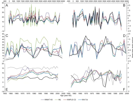
[image:11.595.136.452.62.623.2]when compared to a published reconstruction (Fig. 6A;Amesbury et al., 2008), particularly for ML. However, when viewed as resid-ual plots (Fig. 6B; Swindles et al., 2015b), all models show extremely similar patterns of change over the ~6000 year record. For the simulated shifts in water-table depth (Fig. 6C and D;
Swindles et al., 2015b), all models again produced comparable re-constructions with the exception of ML. All models reconstructed the simulated shifts in water table with the correct frequency and direction of change, but reconstructed shifts were more abrupt, occurring over 2e3 samples, with simulated shifts more gradual, occurring over 6e10 samples. Whereas the wet and dry ends of the simulated shifts were single point extremes, modelled re-constructions exhibited more rapid, threshold-type switches in water table interspersed with plateaux of more consistently wet or dry conditions. Reconstructions of monitored water-table depth at M€annikj€arve fell between the annual and summer mean values for water-table depth (Fig. 6E), but when viewed as residual values (Fig. 6F), differences were evident in the patterns of change over the c. 50 year record, with the comparatively smooth reconstructions suggesting a broadly drier period during the 1970s and 1985e1995, with wetter conditions before and after, whereas instrumental data show that water table varied over shorter time scales throughout the period of monitoring.
All reconstructions were subject to significance testing against transfer functions built on randomly generated data (Table 6;
Telford and Birks, 2011a). This methodology has recently been tested (Payne et al., 2016), with a substantial majority of re-constructions unexpectedly found to be non-significant. In addi-tion, the risks of misapplying (e.g. over-simplified decision making)
or over-relying on (e.g. lack of real-world context)p-value cut-offs, are clear (Wasserstein and Lazar, 2016). However, the significance testing technique does provide a method of statistical assessment that can be used as part of a wider toolkit to evaluate model per-formance. P-values varied between model types and test sets. Only WMAT-K5 reconstructions consistently met thep<0.05 criterion across all test sets. WA-Tol (inv) and WAPLS-C2 reconstructions were consistently p > 0.05, though for the Tor Royal Bog and simulated test sets, were consistentlyp<0.08. ML reconstructions showed the greatest degree of variability, ranging fromp¼0.274 for the Tor Royal Bog test set top¼0.031 for the Mannikj€ €arve test set.
3.4. Spatial scales and regional variability
To further investigate the potential effects of varying spatial scales and supra-regional application on resulting transfer function reconstructions, we subdivided our data into three eco-regions (Fig. 1); Atlantic (n¼461), Scandinavia (n¼341) and Continental (n ¼500). We developed individual transfer functions for each region and applied them to the same three independent test-sets as for the full European-scale models. These three datasets include data from all three eco-regions (Tor Royal Bog in the UK; simulated test set from the UK and Finland; M€annikj€arve from Estonia) so provide a test of the effects in within- and supra-regional model application (Turner et al., 2013). Given the broad similarity of re-constructions between model types (Fig. 6), especially when pre-sented as standardised water-table depth residual values (Swindles et al., 2015b), only one model type (WA-Tol (inv)) was used for this
[image:12.595.49.559.64.390.2]-20 -10 0 10 20 30 40 50 Di ffl ugi a g ra men ty pe P a raqu adrula irregu la ri s Di ffl u gi a o b lo nga ty pe D if flu g ia ac um in a ta t y p e Planocarona (Ne b el a) c a rin a ta ty pe A m ph itrem a w ri g ht ian u m ty pe Ar ce lla h e m isp he ri ca t y pe A rc e lla gi bbo s a ty pe D if flu g ia le id yi Q u ad ru le lla sym m et ri ca A rc e lla v u lg ar is ty pe A rc e lla di s c oi de s t y p e Gibbocarina (Ne b el a) p e na rd ian a ty pe Ar ch er el la f la v u m P lac oc is ta s p in os a ty pe Trac hel eu gly p h a d enta ta t y p e Ar gy nn ia d e n tis to m a t y p e P h ys oc hil a g ris eol a t y p e Ce ntropy x is ac ul ea ta ty pe Sp h e n o de ri a t y p e Di ffl ugi a l u c id a ty pe Hy al os pen ia pap ilio ty pe C y cl o p y x is ar ce lloi de s t y p e Ne bel a c o lla ri s ty p e H e le op e ra p e tr ic ol a ty p e Hy al os phe n ia el eg ans P a da ung iel la la gen ifo rmis ty pe E u gl y p ha c ili ata ty pe Cry p od iffl ug ia s a c c ul us ty pe Ne bel a m ino r Ce ntropy x is ae roph ila ty pe He leo per a sy lv at ic a E u gl y p ha r o tun da ty p e He leo p era r o se a As su lina se mi n u lu m t y p e Hy al os hpen ia su bfl a v a A rc e lla aren aria ty pe Ne bel a fl ab ell u lu m Ne bel a ti nc ta ty p e Longinebela (Ne bel a) m ili ta ri s ty pe Ce ntropy x is ec orn is ty pe As su lina mu sc or um t y p e B u llin ul ar ia in dic a C ryp to di ff lu gi a o v if or m is t y p e C o ry th io n T rin em a ty pe Di ffl ugi a l a bi os a t y p e Trig ono py x is arcula ty pe
W
a
ter
table
depth
(c
m)
Fig. 5.Water-table depth optima and tolerances (cm) for 57 taxa based on the WA-Tol (inv) model after the removal of outlying samples (n¼1302).
exercise. This model type has been frequently applied in previous studies (e.g.Amesbury et al., 2013; Swindles et al., 2015a, 2009) and in this study, compared favourably to other model types in terms of
reported performance statistics, with low RMSEPLOO and
RMSE-PLOSOvalues (Table 5). Performance statistics (RMSEPLOO, R2) for the
regional models (Table 7) were comparable to, or better than, the
-10 0 10 20 30 40 50
-500 0 500 1000 1500 2000 2500 3000 3500 4000 4500 5000 5500 6000
Reconstruc
ted
w
a
ter table depth (cm
)
Age (cal. years BP)
0 5 10 15 20 25 30 35 40 45 50
-2.5 -2 -1.5 -1 -0.5 0 0.5 1 1.5 2 2.5
W
a
ter table
depth
residual
-10 -5 0 5 10 15 20
1955 1960 1965 1970 1975 1980 1985 1990 1995 2000 2005
Age (year AD)
-3 -2 -1 0 1 2 3
1955 1960 1965 1970 1975 1980 1985 1990 1995 2000 2005
WMAT K5 ML WAPLS C2 WA-Tol
-2.5 -2 -1.5 -1 -0.5 0 0.5 1 1.5 2 2.5 3
-500 0 500 1000 1500 2000 2500 3000 3500 4000 4500 5000 5500 6000
A
B
C
D
[image:13.595.41.548.74.458.2]E
F
Fig. 6.Comparison of transfer function reconstructions from four model types (WA-Tol (inv), WAPLS-C2, ML, WMAT-K5) with independent test sets. A, C&E are raw water-table depth values; B, D&F are residual z-scores. A and B: reconstructions from Tor Royal Bog, Dartmoor, UK (Amesbury et al., 2008) compared (panel A only) with a published reconstruction using a European transfer function (black line;Charman et al., 2007). C and D: reconstructions of simulated wet and dry shifts derived from reordered surface samples with associated instrumental water table measurements (black line¼annual mean water-table depth, grey line¼summer (JJA) mean water-table depth;Swindles et al.,
2015b). Y-axis (not shown) is randomly ordered surface sample codes. E and F: reconstructions of near-surface fossil data from M€annikj€arve Bog, Estonia with associated long-term
[image:13.595.29.553.556.601.2]instrumental water table measurements (black line¼annual mean water-table depth, grey line¼summer (JJA) mean water-table depth;Charman et al., 2004).
Table 6
PalaeoSig p values for the significance of reconstructions against models based on randomly generated data for four model types and three independent test sets.
Test set Reference WA-Tol (inv) WAPLS-C2 ML WMAT-K5
Tor Royal Bog Amesbury et al., 2008 0.077 0.075 0.274 0.003
Simulated Swindles et al., 2015a,b 0.051 0.076 0.056 0.011
M€annikj€arve Charman et al., 2004 0.154 0.15 0.031 0.001
Table 7
Summary information and performance statistics for regional transfer function models run using a WA-Tol (inv) model type and the reduced dataset after the removal of outlier samples (n¼1302).
Region n Mean WTD (cm) (range) RMSEPLOO R2(LOO) Average bias (LOO) Maximum bias (LOO)
Atlantic 461 16.0 (-10e52) 8.06 0.60 0.03 20.25
Scandinavia 341 12.7 (-5e50) 7.36 0.53 0.08 15.19
[image:13.595.30.556.699.743.2]full European model (Table 5), potentially suggesting the presence of regional differences in biogeography strong enough to influence model performance. Reconstructed water-table depth profiles for the Atlantic and Continental models for all three independent test sets are broadly similar (Fig. 7) and comparable to the WA-Tol (inv) reconstruction using the full European dataset. However, in all three test sets, the Scandinavian model tended to result in notably different profiles. For the Tor Royal Bog and simulated test sets, the Scandinavian model predicted similar patterns of change but overall wetter conditions (Fig. 7A and B) whereas for the M€annikj€arve test set, drier overall conditions were predicted. The
Scandinavian model contained the lowest number of samples of all three regions (n¼341), but still more than many published models. Scandinavian samples also recorded the highest (i.e. wettest) mean water-table depth of the three regional models (Table 7;Fig. S4; 12.7 cm compared to 16 cm for the Atlantic and Continental models) and the lowest range of water-table depth values (Table 7;
Fig. S4; range of 55 cm, compared to 57 cm and 62 cm for the Atlantic and Continental models respectively).
[image:14.595.146.460.205.705.2]To provide additional insight into the differences between regional models, we examined the prevalence of individual taxa across the three regions to identify whether taxa were
Fig. 7.Comparison of three regional transfer function reconstructions to the full European model for the same three independent test sets asFig. 6. All reconstructions use the WA-Tol (inv) model type. A: Tor Royal Bog (black line uses the established ACCROTELM European transfer function ofCharman et al., 2007); B: simulated changes in water-table depth (black (annual) and grey (summer) lines are instrumental water table measurements); C: M€annikj€arve Bog, Estonia (black (annual) and grey (summer) lines are instrumental water table measurements).
cosmopolitan, or tended to have skewed distributions, favouring a particular region (Fig. 8;Fig. S5). One-way PERMANOVA tests on both individual countries as well as the three eco-regions showed that there were significant differences between both factor coun-tries and regions (p < 0.0001 for both, F¼29.87 for countries, F¼45.6 for regions, assessed by Bray Curtis distance). Twenty-six taxa, including the three most abundant in the dataset (i.e. Assu-lina muscorum(n¼1180),Euglypha ciliatatype (n¼1145),Nebela tinctatype (n¼1022)), were evenly distributed across all sub eco-regions within the wider European study zone (Fig. S5). However, a large number (n¼19) had skewed distributions that suggested taxa were more abundant in particular regions, especially in con-tinental Europe (n¼14;Fig. 8).
4. Discussion
4.1. Data compilation
A low-resolution approach to taxonomy was necessitated in this work by the large number of data contributors (see Methods). It has been shown that reducing taxonomic resolution may have a detrimental effect on model performance (Mitchell et al., 2014; as determined by RMSEP and R2) but with only limited effects on patterns of reconstructed water-table depth. Our data support this view. For example, directional shifts reconstructed by all model types tested showed the same patterns as a European transfer function based on a higher resolution taxonomy (Charman et al., 2007) when applied to a record from Tor Royal Bog, Dartmoor, UK (Fig. 6). Particularly when records were standardised (Swindles et al., 2015b) to remove variability in specific reconstructed water-table depth values (Fig. 6B), the re-constructions at different taxonomic resolutions were indistin-guishable, strongly supporting the view that the necessary reduction in taxonomic resolution applied here has not had a detrimental effect on the potential interpretation of inferred water-table depth profiles from the new model. Indeed, it should be noted that even the highest taxonomic resolution that is practically applicable to light microscopy studies corresponds to a relatively crude resolution in reality given the demonstrated ex-istence of high cryptic and pseudo-cryptic diversity (e.g.Oliverio et al., 2014; Kosakyan et al., 2016), so some degree of taxonomic parsimony will always be necessary.
4.2. Spatial scales and regional variability
The debate surrounding the degree of cosmopolitanism exhibited in free-living microorganisms, of which testate amoebae provide a good model group, is well established and on-going (e.g.
Heger et al., 2009). Conflicting views assume universal ubiquity (Finlay and Clarke, 1999; Finlay et al., 1999, 2001) or (occasional) limited geographical distribution of microorganisms (i.e. the ‘moderate endemicity model’; Foissner, 2008, 2006, 1999). An increasing number of studies focussing on the distribution of testate amoebae have observed taxa which do not appear to sup-port the theory of ubiquity (Smith and Wilkinson, 2007; Smith et al., 2008; Heger et al., 2009, 2011; Yang et al., 2010; Turner et al., 2013; Fournier et al., 2015; Lara et al., 2016).
Europe possesses relatively few of the physical, climatic and biological barriers typically associated with ecological endemism (Kier et al., 2009) and the passive distribution of testate amoebae should, therefore, be comparatively uninhibited. As a result, it could be argued that any evidence of regionally restricted distributions of testate amoebae in Europe, which cannot be explained by other ecological factors, such as peatland type and trophic status, is supporting evidence of the moderate endemicity model.
By compiling data from across Europe, we were able to examine the distributions of taxa across the continent. The ma-jority (41 of 47) of taxa were found in all regions (Fig. 8andS5), arguing strongly that the continental transfer function can be readily applied to individual core locations within its geograph-ical extent. The Continental region was the most taxonomgeograph-ically diverse, with only Nebela flabellulum (strongly skewed to the Atlantic region; Fig. 8) completely absent. A similar strongly oceanic distribution has been noted for this taxon in Canadian peatlands (Charman and Warner, 1997), which was the most common to be completely absent from any one region (n¼246 samples). Three taxa were present only in the Continental region, being completely absent from both the Atlantic and Scandinavian regions (Centropyxis ecornis type, Difflugia gramen type, Para-quadrula irregularis), however these were rare taxa, with C. ecornistype the most common (n¼26;Fig. 8) andD. gramen andP. irregularisnever occurring>5% in any one sample (n¼1 and n¼2 respectively). In addition,P. irregularisis a calcareous taxon found predominately in rich fens (e.g.Lamentowicz et al., 2013a), which were mainly sampled in the Continental region and were included in the model due to having no associated pH measurement.Difflugia labiosatype was absent from the Atlantic region and present at very low abundance (0.7%) in only one sample in the Scandinavian region.Arcella hemisphaericatype was completely absent from the Atlantic region, whereasAmphitrema wrightianumtype was strongly skewed towards it, also in com-mon withfindings from Canada (Charman and Warner, 1997). For nutrient poor, ombrotrophic peatlands, given the number and range of sites included in the dataset, it is likely that these regional patterns represent genuine geographical restrictions of these taxa, rather than a lack of appropriate habitats (Smith and Wilkinson, 2007; Smith et al., 2008; Yang et al., 2010). Patterns relating to taxa commonly associated with other site types (e.g. rich fens; P. irregularis, Lamentowicz et al., 2013a) should be viewed with more caution since only limited numbers of geographically restricted samples from such site types were included in the model as a result of their lacking associated pH measurements.
02
0
4
0
6
0
ARC ARE (537)
%
abundanc
e
04
0
8
0
ARC DIS (332)
02
0
4
0
6
0
ARC VUL (68)
01
0
3
0
BUL IND (275)
0
1
03
05
0
CEN ACU (206)
051
0
1
5
CEN ECO (26)
0246
8
DIF LAB (9)
02
0
4
0
6
0
HEL PET (560)
%
abundanc
e
1 2 3
02
0
6
0
HYA PAP (626)
1 2 3
02
0
4
0
6
0
HYA SUB (99)
1 2 3
0
5
10
15
GIB PEN (43)
1 2 3
02
0
4
0
PSY GRI (369)
1 2 3
05
1
0
1
5
QUA SYM (19)
1 2 3
02
0
4
0
6
0
TRA DEN (57)
1 2 3
02
0
6
0
AMP WRI (179)
02
0
4
0
6
0
NEB FLA (246)
01
0
2
0
3
0
ARC HEM (57)
02
0
4
0
6
0
NEB COL (230)
0
5
15
25
PLA SPI (198)
%
abundanc
e
Skewed to Region 3
Skewed to Regions 2 & 3
Skewed to Region 2
[image:16.595.65.718.138.434.2]Skewed to Region 1
Fig. 8.Taxa with uneven distributions across the three regions (n¼19). Taxa with all occurrences<5% abundance have been excluded (n¼2; DIF GRA and PAR IRR). Region codes on x-axes: 1¼Atlantic, 2¼Scandinavia, 3¼continental Europe. For full taxa abbreviations, seeTable 2. Number of occurrences in 1302 samples shown in brackets after taxon code. Red dots indicate complete absence from a particular region. (For interpretation of the references to colour in thisfigure legend, the reader is referred to the web version of this article.)
M.J.
Amesbury
et
al.
/
Quaternary
Science
Reviews
15
2
(20
16
)
132
e
151
14
The use of local transfer functions to reconstruct water-table depth from other regions should be approached with caution (Turner et al., 2013), but by including a high number of analogues from a wide geographic region and long water table gradient and by using a relatively coarse taxonomic resolution, we show here that continental-scale models may be just as effective in reconstructing local changes as local-scale models specific to the core data loca-tion. A large scale regional model such as that presented here will contain more analogues and therefore provide a more robust approach to reconstructing past hydrological variability than the use of smaller data sets collected from individual sites or small regions.
4.3. A way forward for interpreting transfer function-based palaeohydrological reconstructions?
Due to the complexity of peatland water table and testate amoeba ecological responses, both moderated by a range of differing factors, it is becoming clear that transfer function re-constructions should not be seen as simple metrics of past climate (Turner et al., 2013). In addition, the apparent inaccuracy of reconstructed water-table depth values, particularly towards the ‘dry’end of the gradient where both methodological and ecolog-ical problems are exacerbated, suggests that reconstructions should be displayed as residuals or standardised values and interpreted primarily as metrics of directional shifts between wetter and drier conditions, an approach in which context re-constructions from a range of models have shown to be robust (Swindles et al., 2015b). Our own data (e.g. Figs. 6 and 7) show that, with some exceptions, our models are relatively consistent in performance for reconstructed water-table depth values across the full gradient. This is likely as a result of the high number of samples characterising all water table segments (Fig. S2); although there are relatively fewer samples in drier water table segments, a common problem identified in other studies (Amesbury et al., 2013; Swindles et al., 2015a). Segment-specific n values are still high (lowest is n¼25 for 45e49.5 cm, mean for all water-table depth segments>20 cm is n¼70), highlighting the value of the large compiled dataset. However, the variability present between both model types and regions, despite an unprecedented training set size, argues that reconstructions should be standardised and presented as residual values (sensuSwindles et al., 2015b) in order to focus interpretation on secure directional shifts, avoiding potentially inaccurate conclusions relating to specific water-table depths.
There has been a recent recognition that testing transfer functions against independent instrumental data may be a more powerful test than relying purely on statistical methods (Swindles et al., 2015b). Here, by applying both approaches, we are able to rigorously validate our new models and show that, despite a low-resolution taxonomic approach, our new pan-European transfer function provides a reliable tool for recon-struction of Holocene hydroclimatic shifts across Europe. In particular, we highlight the potential limitations of applying statistical tests alone. The use of the‘randomTF’function, which tests the significance of reconstructions against models trained on randomly generated data has recently been reviewed (Payne et al., 2016), with >80% reconstructions tested found to be insignificant (p>0.05), with no correlation between significance and model performance. Our results question the efficacy of this method as different model types applied in different regions (Table 6) showed only 4 out of 12 ‘significant’ reconstructions and resulted in a range ofpvalues from 0.001 to 0.274, despite all reconstructions being trained on the same data and showing
what could be interpreted as the same reconstructed patterns of change (Fig. 7). Coupled with recent guidance that warns against the use of seemingly arbitraryp-value cut-offs and stresses the need for contextual information in decision making rather than a binary‘yes/no’approach (Wasserstein and Lazar, 2016), a multi-faceted approach to model assessment is clearly supported. While statistical validation remains an important and useful in-dicator of model performance alongside tests against indepen-dent data, we advocate a balanced approach to model efficacy taking into account both lines of evidence as well as the role of contextual information. For example, some ‘insignificant’ re-constructions (Table 6) performed well in tests against inde-pendent data (Fig. 7). In addition, the similarity of reconstructions across model types and/or regions presented here (Figs. 6 and 7), despite variations in performance statistics, suggests that the high number of training set samples has resulted in a wider range of modern analogues and therefore a better representation of testate amoeba ecology in the model.
5. Conclusions and guidelines for the application of the transfer function
We developed and validated a new pan-European peatland testate amoeba-based transfer function for palaeohydrological reconstruction using a vastly expanded dataset of 1799 samples and a newly developed low resolution taxonomic scheme to accommodate the large number of data contributors. Following the removal of samples with high pH values, we developed water-table depth transfer functions using a range of model types. These were tested using a combination of statistical validation and comparison to independent test sets with associated instrumental water table measurements. Taxonomic resolution did not impair model performance, which was comparable to other published models. We conclude that the new model provides an effective tool for testate amoeba-based palaeohydrological reconstruction in ombrotrophic peatlands throughout Europe. Model output should be standardised and presented as residual values to focus interpretation on directional shifts and avoiding potential misin-terpretation of absolute water-table depth values. The extent and diversity of the dataset highlighted that, at the taxonomic reso-lution applied, a majority of taxa had broad geographic distribu-tions, though some morphotypes appeared to have restricted ranges.
To facilitate future research, we provide the full compiled dataset, along with R code to allow the free application of our transfer function to fossil data by individual users, as supplemen-tary online material. The R code facilitates the application of the WA-Tol (inv) model and conversion of reconstructed water-table depth values to standardised residual z-scores. The WA-Tol (inv) model type has been commonly applied in other studies (e.g.
Amesbury et al., 2013; Swindles et al., 2015a, 2009) and compared favourably to other model types in terms of reported performance statistics in this study. Users are free to alter the R code as appro-priate to apply other model types, but should justify these changes in their work.
Author contributions