Underwater glider navigation error compensation using sea current data

This is a repository copy of Underwater glider navigation error compensation using sea

current data.

White Rose Research Online URL for this paper:

http://eprints.whiterose.ac.uk/144679/

Version: Accepted Version

Proceedings Paper:

Kim, J orcid.org/0000-0002-3456-6614, Park, Y, Lee, S et al. (1 more author) (2016)

Underwater glider navigation error compensation using sea current data. In: IFAC

Proceedings Volumes. 19th IFAC World Congress, 24-29 Aug 2014, Cape Town, South

Africa. Elsevier , pp. 9661-9666. ISBN 9783902823625

https://doi.org/10.3182/20140824-6-ZA-1003.01508

© 2014, Elsevier. This manuscript version is made available under the CC-BY-NC-ND 4.0

license http://creativecommons.org/licenses/by-nc-nd/4.0/.

[email protected] https://eprints.whiterose.ac.uk/

Reuse

This article is distributed under the terms of the Creative Commons Attribution-NonCommercial-NoDerivs (CC BY-NC-ND) licence. This licence only allows you to download this work and share it with others as long as you credit the authors, but you can’t change the article in any way or use it commercially. More

information and the full terms of the licence here: https://creativecommons.org/licenses/

Takedown

If you consider content in White Rose Research Online to be in breach of UK law, please notify us by

Underwater glider navigation error

compensation using sea current data

⋆

Jongrae Kim∗ _{Yosup Park}∗∗ _{Shinje Lee}∗∗ _{Yong Kuk Lee}∗∗

∗

Biomedical Engineering/Aerospace Sciences, University Avenue, University of Glasgow, Glasgow G12 8QQ, UK (e-mail:

[email protected]). ∗∗

Korea Institute of Ocean Science & Technology, 787 Haean-ro, Sangnok-gu, Ansan-si, Gyeonggi-do, Republic of Korea (e-mail: yosup,

sinje, [email protected])

Abstract: Underwater glider is an emerging platform to explore the ocean with remarkably

long operational endurance up to several months. Underwater glider navigation systems have significant limitations, on the other hand, in keeping the navigation error small. There is no reference coordinates information for position estimation and not enough immediate orientation reference for attitude estimation under the sea. Moreover, external disturbances including the sea currents make the navigation error increase further. In order to reduce the navigation error, we exploit a priori knowledge on the average current over the operation area. The performance and the robustness of the proposed algorithm are demonstrated using an experimental data obtained by Korea Institute of Ocean Science & Technology. The algorithm can be used to reduce the navigation error for one glider and also for multiple gliders by fusing the estimated errors. It can be also directly used to predict floating object path in order to use the prediction to design a collision avoidance path.

Keywords:Underwater Glider, Navigation Error, Floating Object, Collision Avoidance

1. INTRODUCTION

There has been a growing awareness of the ocean’s roles in our life over the past few decades. In expanding our capa-bilities to acquire the knowledge of the world’s oceans, the traditional observation platforms, for example, ships and mooring systems, have shown some limitations, which stem from high operation cost and some safety issues (Eriksen et al., 2001). On the other hand, UUV (Unmanned Un-derwater Vehicle) has proven to be an efficient tool for offshore resources exploration, maritime management, and naval defence with a lot less operation cost and almost free from any safety issues.

Two typical types of UUV are the one using screw pro-pellers and the one using environmental energy, e.g., wave, wind, buoyancy gravity. UUV with propellers has ac-curate navigation capability and horizontal manoeuvra-bility but its operation time and the range are rather short, a few hours and less than 100km. UUV without propeller is called autonomous underwater glider. It has the global navigation and the vertical profiling manoeu-vring capabilities with the monthly operation time and the long range over 1000km. Underwater gliders have clear advantages over the profiling floats because of active position control. Underwater gliders perform saw-tooth

⋆ _{This research was supported by Research on Automatic Control} Technology of Underwater Glider, which is supported by DAPA (Defense Acquisition Program Administration, KOREA). The first author’s research is also supported by EOARD (European Office of Aerospace Research & Development), the grant number US-EURO-LO (FA8655-13-1-3029).

trajectories from the surface to depths of 1000-1500m, along re-programmable routes using two-way communica-tion via satellite. They can reach the forward speeds up to 40km/day, thanks to wings and rudders, and can be operated for a few months before they have to be recovered (Davis et al., 2002; Griffiths et al., 2001).

Gliders can record physical quantity, e.g., temperature and salinity, and biogeochemical quantity, such as pH, oxygen, and nitrate. At each surfacing, the collected data is sent to the land operation centre and new commands are received, if necessary, via the bidirectional Iridium satellite communication system at the rate of 30 to 60Kbytes for 5 minutes in every 4 to 5 hours. Underwater glider has so many advantages including long term mission, controlled navigation, profiling capabilities, easy deploy & recovery operation, and satellite communication. They could be used to monitor key regions in the world, where one needs to collect data with a higher resolution than presently available (Testor et al., 2009).

[image:3.595.340.522.69.147.2]

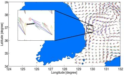
Fig. 1. The experiment was performed in East Sea in-dicated by the rectangular box. The arrows are the average current velocity at each location for seven different dates from 11th to 17th March of 2011 (Ko-rea Hydrographic & Oceanographic Administration, 2011). The red circles in the inset box are the position information from GPS and the black thick line is the path obtained by the estimator designed in Section 3.

be completed and the position is obtained by correcting the acceleration measurement further using an average sea current velocity data.

KIOST (Korea Institute of Ocean Science & Technology) has been operating underwater gliders since 2011. The first flight was crossing East Sea during 6 days, where the eddy current of 1kt was present, and touching down 200m depth while sound velocity and temperature profiling at every 5 seconds (Imlach and Mahr, 2012; Park et al., 2012). All the experimental data presented in the following were obtained during this operation in the region shown in Figure 1 using Exocetus Coastal Glider, LG19 (Exocetus, 2013; Imlach and Mahr, 2012). Its diameter and length are 32.4cm and 2.87m, respectively, and its weight is 109kg. It is equipped with an IMU (Inertial Measurement Unit), which provides heading, roll and pitch angles, position, velocity, and acceleration of the glider.

In the following, Section 2, the navigation equation is derived and the navigation sensor output is characterised. In Section 3, the major navigation error sources are mod-elled and the error correction algorithms using the built-in navigation system output and the average sea current data are presented. The performance of the algorithms are demonstrated using a field data collected by KIOST. Finally, the conclusions are presented.

2. NAVIGATION SYSTEM

2.1 Relative Motion Equation

The relation among the position vector of the underwater

glider,rb, the sensor position in the body-coordinates (B),

rs, and the one in the reference-coordinates (R), r, is

shown in Figure 2 and given by

r=rb+rs (1)

More explicitly with the coordinates expressed,

rb=r

B

−rB_s (2)

whererbis the position vector expressed by two vectors in

the right hand side, andBin the superscripts is indicated

that both vectors are expressed in the body-coordinates.

Fig. 2. The origins of the reference-coordinates and the

body-coordinates are indicated by O and B,

respec-tively. The body coordinates is attached to the glider

and rs is the sensor position vector relative to the

origin of the body-coordinates.g is the gravitational

acceleration vector.

Take the time-derivative of (2) and obtain the velocity,

vb =

d dtrb=

d dtr

B

−ω×rB_s (3)

where ˙rB

s is zero because the glider is assumed to be a

rigid-body, and the following transport theorem is used in the derivative (Schaub and Junkins, 2009).

Theorem 1. (Transport Theorem) The time derivative of

a generic vector, x, which is expressed in the rotating

coordinates with the angular velocity, ω, with respect to

the inertial coordinates is

dR dtx

B

=d

B

dtx B

+ωB×xB

or simply

dR

dtx= ˙x+ω×x (4)

where×is the vector cross product.

Proof:The proof is omitted and it can be found in (Schaub

and Junkins, 2009).

Note that the first term in the right-hand side of (3) is not expanded using the Transport theorem. Later, it will be

directly obtained from the accelerometer attached atrsin

the glider.

Take one more time-derivative of (3)

ab=

d dtvb=

d2

dt2r−ω˙ ×rs−ω×(ω×rs) (5)

where the superscript, B, in the terms in the right hand

side is dropped for brevity, and they are all expressed in the body-coordinates.

2.2 Navigation Equation

The following quantity,aB

acc, can be measured by the 3-axis

accelerometer in the glider: aBacc= ¨r+C

B

R(ψ, θ, φ)g R

(6)

where aBacc is the acceleration information expressed in

the body-coordinates, ¨ris equal tod2

r/dt2

,CB

R(ψ, θ, φ) is

the direction cosine matrix, which changes the coordinates from the reference to the body with the rotating sequence

given by yaw(ψ), pitch(θ), and roll(φ), gR

= [0,0,−g]T_, the gravitational acceleration expressed in the reference

coordinates, andg= 9.821 m/s2

.

Substituted2

r/dt2

in (5) by the expression in (6)

ab=

d dtvb=a

B acc−C

B Rg

R

−ω˙ ×r_s−ω×(ω×r_s) (7)

19th IFAC World Congress

Cape Town, South Africa. August 24-29, 2014

[image:3.595.62.271.70.198.2]

0 20 40 60 80 100 120 140 160 180 10−10

10−8

10−6

10−4

time [minutes]

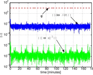
[image:4.595.90.240.72.193.2]

||.|| _||[ωx]2||

Fig. 3. The norms of angular acceleration and squared angular velocity cross product operator are about 100 times or 100 million times smaller than the gravitational acceleration.

In a matrix operation format, it can be written as

ab=

d dtvb =a

B acc−C

B Rg

R

−[ ˙ω×]r_s−[ω×]

2

rs (8)

where

[ω×] :=

" _{0 −ω3 ω2}

ω3 0 −ω1

−ω2 ω1 0

#

, (9)

ωi for i = 1,2,3 is the angular velocity for each axis in

the body-coordinates, and [ ˙ω×] is defined in the similar

manner.

Rotational angular velocity of underwater vehicle is, in

general, very slow, i.e.kωkandkω˙kare much smaller than

kgk. Figure 3 shows that in the experiment the magnitudes

of two terms are at least 100-times smaller than the magnitude of the gravitational acceleration. Note that the angular acceleration is calculated by finite-difference using

the angular rate measurement. In addition, krsk is less

than 1m and kCB

Rk is equal to 1. Hence, the angular

velocity related terms in (8) can be ignored and the acceleration becomes

ab≈aBacc−C

B Rg

R

(10)

After transforming the coordinates of (10) into the reference-coordinates, integrating it with respect to time provides the velocity expressed in the reference frame as follows:

vR_b (t) =CBR(t0)v B

b(t0) +

Z t

t0

CBR(τ)a B

b(τ)dτ (11)

where t0 is the initial time,CR

B(t0) is the initial attitude,

vB

b(t0) is the initial velocity, and in order to emphasise the

dependency to time each term in the above is written as a

function of time. Note thatCR

B is equal to the transpose

ofCB

R.

Finally, the glider position in the reference frame is ob-tained by

rR_b (t) =rR_b (t0) +

Z t

t0

v_bR(τ)dτ (12)

whererR

b (t0) is the initial position of the glider.

2.3 Navigation Algorithm & Sensor Output

Exocetus Coastal glider has a built-in navigation algo-rithm and it records various navigation data. The following

as follows: ˜

aacc= ˜¨r+CB_R(ψ, θ, φ)gR+bacc+nacc (13)

where ˜¨r is the measured quantity by the calibrated

ac-celerometer if there is no stochastic noise and bias error,

baccis the accelerometer sensor bias error,naccis the white

noise, and the accelerations caused by the control forces

and the external disturbances are all included in ¨r. Usually,

in the estimation problem, ˜¨r is assumed to equal to ¨r,

which presumes infinite resolution and infinitesimal time constant, i.e. a perfect sensitivity. In reality, including the limitations in the resolution and the finite response time,

and some unknown error sources, ˜¨rwill be different from

¨

r(Ulanov, 2006).

The navigation algorithm provides the attitude

informa-tion, which includes some errors,δψ, δθ, andδφ, then

CB R=C

B

B′(δψ, δθ, δφ)C B′

R( ˜ψ,θ,˜ φ˜) (14)

where B′

is the body-coordinates that the navigation

system calculated, ˜ψ,θ,˜ φ˜ are roll, pitch and yaw angles

returned from the navigation algorithm, andδψ, δθ, δφare

the attitude angles of the true body-coordinates,B, with

respect to the calculated body-coordinates,B′_{. With the}

small angle assumption, i.e.,δψ≪1,δθ≪1, andδφ≪1,

CB

B′(δψ, δθ, δφ)≈

" _{1 δψ δθ}

−δψ 1 δφ

δθ −δφ 1 #

(15)

In addition, the navigation system log-file provides the velocity and the position estimations in the reference

coordinates, i.e., ˆvR

b (t) and ˆr

R

b (t).

3. NAVIGATION ERROR REDUCTION

There are three major error sources in the acceleration

esti-mation: physical sensor limitation in the accelerometer(Ƭr);

orientation error (∆C); and the accelerometer bias (bacc).

The detail algorithm of the glider navigation system is unknown but in general the orientation error can be kept quite small. The glider has the magnetometer and it could provide reasonably good heading information. Moreover, whenever the angular velocity remains roughly constant during a certain time interval, then the direction of the gravitational vector can be estimated. Using these two vectors, the standard orientation estimation algorithm, e.g. QUEST (Quaternion Estimation) (Shuster and Oh, 1981), with Kalman Filter (Lefferts et al., 1982), would work very well in minimising the attitude estimation error.

Hence, the navigation system returns reasonably accurate

orientation information, CB

B′ ≈ I3, where I3 is the 3x3

identity matrix. For example, the Slocum glider attitude

error is around±1◦

in heading accuracy and±0.2◦

in roll and pitch accuracy (Smith et al., 2010). In addition, the

accelerometer sensor bias,bacc, would be well-estimated a

0 20 40 60 80 100 120 140 160 180 −10 −8 −6 −4 −2 0 2 4 6 time [minutes]

Accelerometer Raw Output [m/s

2]

a x a_y

[image:5.595.359.505.70.186.2]

a_z

Fig. 4. Raw accelerometer measurements output

0 20 40 60 80 100 120 140 160 180

−0.5

0 0.5 1

[m/s]

0 20 40 60 80 100 120 140 160 180

−0.5

0 0.5 1

[m/s]

0 20 40 60 80 100 120 140 160 180

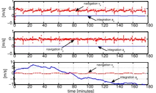
−10 −5 0 5 10 time [minutes] [m/s] integration a x integration a y integration a z navigation vx

navigation v y

navigation v z

Fig. 5. Comparison between the integration of the ac-celerometer measurements output and the velocity information from the navigation system

but the raw measurement including the gravitational

ac-celeration. Therefore,baccand Ƭrare the unknowns to be

estimated.

In the following, firstly, we estimate the bias in the acceleration measurement using the navigation system

output and secondly, Ƭrwill be reduced using the average

sea current data. The performance of the algorithms will be verified using the GPS updated position information.

3.1 Accelerometer Error Model

The acceleration of the glider, (10), is calculated as follows:

ˆ ab = ˜a

B acc−C

B′

Rg R

(16)

where the raw measurement from the experiment, ˜aBacc, is

shown in Figure 4.

The error between (10) and (16) is defined by

δab= ˆab−ab= ∆¨r+ ∆C gB ′

+bacc+nacc (17)

where

∆¨r= ˜¨r−¨r (18)

∆C=

" _{0 δψ δθ}

−δψ 0 δφ

δθ −δφ 0 #

, (19)

gB′ is the gravitational acceleration expressed in B′

, and

δψ, the yaw angle error does not affect to the projection

of the gravitational vector on the body-coordinates (B′

). Hence,

gB′ =g

−sin ˜θ,sin ˜φcos ˜θ, cos ˜φcos ˜θT

(20)

where (·)T _{is the transpose of the vector.}

0 20 40 60 80 100 120 140 160 180

−0.2 −0.1 0 0.1 0.2 ax [m/s 2]

0 20 40 60 80 100 120 140 160 180

−0.2 −0.1 0 0.1 0.2 ay [m/s 2]

0 20 40 60 80 100 120 140 160 180

[image:5.595.89.241.72.200.2]

−1 −0.5 0 0.5 1 time [minutes] az [m/s 2]

Fig. 6. Bias corrected acceleration measurement

0 20 40 60 80 100 120 140 160 180

−0.5 0 0.5 1

[m/s]

0 20 40 60 80 100 120 140 160 180

−0.5 0 0.5 1

[m/s]

0 20 40 60 80 100 120 140 160 180

−1 −0.5 0 0.5 1 time [minutes] [m/s]

integral a_y

navigation v_y integral a_x

navigation v_x

integral a_z

navigation v_z

Fig. 7. Comparison between the integration of the cor-rected acceleration and the velocity information from the navigation system

3.2 Error Correction Using Navigation Data

If the accelerometer output is directly integrated after the gravitational effect is removed using the attitude information, the velocity is still very different from the one from the navigation system as shown in Figure 5.

Using the accelerometer output, the velocity can be writ-ten as follows:

˙

v=CBRab=C

R B′C

B′

B (ˆab+δab)

=CR

B′(I+ ∆C) (ˆab+δab) (21) and it can be further expanded

˙

v=CR

B′(ˆab+ ∆Cˆab+δab+ ∆Cδab) (22) Let

w=−CR

B′(∆Caˆb+δab+ ∆Cδab) (23) then,

˙

v=CR

B′ˆab−w (24)

Assume w be approximated as a piecewise constant, i.e.,

the following is satisfied almost every instant: ˙

w≈0 (25)

Hence, the navigation equation for each axis is given by ˙

x=Ax+Bu (26)

whereuis thei-axis component ofCR

B′ˆab,

x= [pi vi wi] T

(27)

for i =x, y or z, pi is the i-axis coordinate of the glider

in the reference frame, vi is the i-axis velocity of the

glider in the reference frame, wi is the i-axis error in

the accelerometer measurement projecting on the reference frame, and

A=

"_{0 1 0}

0 0 −1

0 0 0 #

, B=

"₀

1 0 #

(28) 19th IFAC World Congress

Cape Town, South Africa. August 24-29, 2014

[image:5.595.344.511.213.312.2] [image:5.595.87.247.234.329.2]

Longitude [degree]

Latitude [degree]

129.8 129.85 129.9 129.95 130 36.7

36.75 36.8 36.85

[image:6.595.353.508.71.185.2]

Initial Position

Fig. 8. Paths obtained by integrating the bias error only (black solid line), and the bias with the sea current drag fixed (red dashed line) accelerometer measure-ment. Initial and the final position update using GPS are indicated by the red circles and the coloured ar-rows are the average current for seven different dates. Hence, the corresponding estimator is

˙ˆ

x=Axˆ+Bu+Kobs(Cxˆ−y˜) (29)

whereKobs is the observer gain to be designed,

C=

1 0 0 0 1 0

, y˜=

pnavi

vnav

i

(30)

and pnav

i and v

nav

i are the position and the velocity

information ofi-axis from the navigation system. In order

to make the error dynamics of the estimator stable, i.e., the

real parts of all eigenvalues of A+KobsC being negative,

the following gain is chosen by trial and error:

Kobs=−5

"_{1 1}

0 1

0 −1

#

(31)

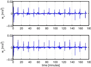
Using w from the estimator, (29), the acceleration, ˙v,

is calculated from (24) and it is shown in Figure 6. In order to verify whether these acceleration would be close to the true, the acceleration is numerically integrated and it provides the velocity. The velocity is compared with the velocity information from the navigation system in Figure 7. As shown in the figure, two quantities are almost identical and we can conclude that the acceleration calculated is at least as much accurate as the acceleration information that the navigation system has.

3.3 Error Correction Using Average Sea Current

Once the bias correction is completed, the position in-formation can be obtained by integrating the corrected accelerometer output twice. The integrated path is shown in Figure 8 indicated in the black solid line. The starting position was initialised by the GPS signal and it has an accurate starting position information. However, because

of Ƭr error effects accumulated during the diving, the

position at the end just before it is updated by GPS again has several km error after about 3 hours operation under the water, as shown in Figure 8. The main cause of this error might be the current as the final position is almost exactly drifted towards the directions where the average current flows. The similar drifts are observed in another three diving (Alaks Native Technologies, 2011).

The question is why the force caused by the current is not included in the accelerometer measurement. To quantify how much acceleration would be generated from

0 20 40 60 80 100 120 140 160 180

−0.02

0 20 40 60 80 100 120 140 160 180

−0.02

0 0.02

wy

[m/s

2]

time [minutes]

Fig. 9. Acceleration in the East and the North directions caused by the current drag force

the current, the following equation is used (Sherman et al., 2001):

D=1

2ρk∆vk

2

ADCD (32)

where ρ is the sea water density, which is around 1020

kg/m3

, ∆v is the relative velocity of the glider in the

horizontal plane, i.e.

∆v=

vcrt E v

crt N 0

T

−[vx vy 0]

T

, (33)

vcrt

E and v

crt

N are the sea current velocity in the east

or the north direction, respectively, whose magnitude is

around 1kt (≈0.5 m/s) in the maximum,AD is the cross

section area of the glider hull, which is about 824 cm2

,

andCD is the drag coefficient set to 0.4, which is adopted

from (Sherman et al., 2001). Unlike the example shown in (Sherman et al., 2001), the glider has a small wing and the induced drag is ignored. The drag is about 4N with the

values in the above whenv= 0 and it corresponds to the

acceleration of 0.04 m/s2

(≈4N/109kg). The acceleration,

0.04 m/s2

, is the possible maximum value when the glider is stationary. The acceleration caused by the current would be much smaller than the maximum as the glider usually does not fly in the exact opposite to the current. Then, these tiny current effect would be completely blocked by the sensor noise and the external fluctuations.

After the bias error in (23) is corrected in the previous section, given that the attitude error is small compared to the bias and the current effect on the acceleration measurement, the remaining uncorrected error in (23) is

w≈ −CBR′∆¨r=

D

meD (34)

where m is the mass of the glider and eD is the unit

vector towards the current direction. Sea current near the surface is mainly caused by wind and the temperature differences. Hence, the vertical direction is negligible in the near surface depth compared to the magnitudes of the horizontal direction components (Park et al., 2013). Hence,

eD=





 ∆v

k∆vk, fork∆vk>0

0, otherwise

(35)

[image:6.595.95.238.71.190.2]

Table 1. Final position error ([km]) for the bias only fixed (B) and the bias with the sea current

fixed using seven different current data

Day 1 2 3 4 5 6 7 B

Err 2.73 2.73 2.73 2.73 2.73 2.72 2.72 4.85

The path comparison between the one obtained by inte-grating the bias fixed only acceleration and the one by integrating the bias and the sea current fixed acceleration is shown in Figure 8. The total distance is shortened about 30% but the direction is correctly pointing toward the final position provided by GPS. The paths calculated using different current data are compared in Table 1 in terms of the distance from the estimated at the final and the one from GPS. The error reduced about 43% compared to the one without the current drag compensation.

4. CONCLUSIONS & FUTURE WORKS

Algorithms to correct various errors in the accelerometer output of underwater glider are presented. The algorithms do not require to investigate the built-in navigation sys-tems of the glider, which is normally provided by the man-ufacturer or already installed on the glider. The algorithm corrects the bias error using the navigation system output and corrects further using the a priori information about the average current data over the operation area. The cal-culation results using the experimental data collected by KIOST in East Sea, Korea, demonstrate the performance of the algorithms.

The uncertainty boundary of the final GPS update po-sition could be obtained by providing the ranges of sev-eral physical parameters, e.g., drag coefficient, mass, sea current changes, etc. The proposed algorithms can be implemented in on-board computer without requiring too much computational power. Moreover, for the case without having the current information, it can be still used recur-sively by estimating the current based on the position error measured every diving. Finally, the proposed algorithm could be used the predict the path of floating objects and the prediction would be exploited in the glider path planning to avoid any collision.

Although the algorithm shows some robustness towards the uncertainties in sea current data, it is, however, ideal to have more accurate and up to date information. In future, some real-time current data, e.g. OSCAR (Ocean Surface Current Analysis - Real time) project (National Oceanic and Atmospheric Administration, 2013), would be avail-able and this could improve the algorithm performance in reduction the navigation error.

ACKNOWLEDGEMENTS

This research was supported by Research on Automatic Control Technology of Underwater Glider, which is sup-ported by DAPA (Defense Acquisition Program Admin-istration, KOREA). The first author’s research is also supported by EOARD (European Office of Aerospace Research & Development), the grant number US-EURO-LO (FA8655-13-1-3029). The authors would like to thank Mr. Yang Sik Baek from ADD (Agency for Defense Devel-opment) for his continued support of the glider develop-ment.

REFERENCES

Alaks Native Technologies, L. (2011). ANT analysis of KORDI LG19 flight. Technical Memo.

Davis, R.E., Eriksen, C.C., and Jones, C.P. (2002). The

Technology and Applications of Autonomous Under-water Vehicles, chapter 2, Chapter 3. Autonomous Buoyancy–driven underwater gliders. Taylor & Francis. Eriksen, C.C., Osse, T.J., Light, R.D., Wen, T., Lehman, T.W., Sabin, P.L., Ballard, J.W., and Chiodi, A.M. (2001). Seaglider: a long-range autonomous underwater

vehicle for oceanographic research. Oceanic

Engineer-ing, IEEE Journal of, 26(4), 424–436.

Exocetus (2013). Exocetus. URLhttp://exocetus.com.

Griffiths, G., Davis, R., Erikson, C., Frye, P., Marchand, T., Dickey, T., and Weller, R. (2001). Towards new

platform technology for sustained observations. InFirst

International Conference on Ocean Observations for Climate (OCEANOBS99), 324–337.

Imlach, J. and Mahr, R. (2012). Modification of

a military grade glider for coastal scientific

ap-plications. In Oceans, 2012, 1–6. IEEE. doi:

10.1109/oceans.2012.6405134.

Korea Hydrographic & Oceanographic Administration (2011). East sea surface currents prediction model. Lefferts, E.J., Markley, F.L., and Shuster, M.D. (1982).

Kalman filtering for spacecraft attitude estimation.

Journal of Guidance, Control, and Dynamics, 5(5), 417– 429.

National Oceanic and Atmospheric Administration (2013). OSCAR near realtime global ocean surface currents.

URLhttp://www.oscar.noaa.gov.

Park, Y., Lee, S., Lee, Y., Jung, S.K., Jang, N., and Lee, H.W. (2012). Report of east sea crossing by underwater

glider. Journal Of the Korean Society of Oceanography,

130–137.

Park, Y.G., Park, J.H., Lee, H.J., Min, H.S., and Kim, S.D. (2013). The effects of geothermal heating on the

East/Japan Sea circulation. J. Geophys. Res. Oceans,

118(4), 1893–1905. doi:10.1002/jgrc.20161.

Schaub, H. and Junkins, J. (2009). Analytical Mechanics

of Space Systems (AIAA Education Series). AIAA, 2 edition.

Sherman, J., Davis, R., Owens, W.B., and Valdes, J. (2001). The autonomous underwater glider ”Spray”.

Oceanic Engineering, IEEE Journal of, 26(4), 437–446. doi:10.1109/48.972076.

Shuster, M.D. and Oh, S.D. (1981). Attitude

determi-nation from vector observations. Journal of Guidance,

Control, and Dynamics, 4(1), 70–77.

Smith, R.N., Kelly, J., Chao, Y., Jones, B.H., and Sukhatme, G.S. (2010). Towards the improvement of autonomous glider navigational accuracy through the

use of regional ocean models. In Proc. ASME 2010

29th Int’l Conf. Ocean, Offshore and Arctic Engineering (OMAE’10). Shanghai, China.

Testor, P., Meyeres, G., and et. al. (2009). Gliders as a

component of future observing systems. InProceedings

of the OceanObs’09: Sustained Ocean Observations and Information for Society Conference (Vol. 2).

Ulanov, A.V. (2006). Underwater glider navigation

in a nonhomogenous current. Aerospace and

Elec-tronic Systems Magazine, IEEE, 21(11), 27–28. doi: 10.1109/MAES.2006.284355.

19th IFAC World Congress

Cape Town, South Africa. August 24-29, 2014