Mössbauer effect study of the paramagnetic hyperfine structure of K₃[(Al₁ˍₓFeₓ)(C₂O₄)₃].3H₂O

P A R A

M A G N

E T I C H Y

P E R F I N E

S

T R U C T U R E

MOSSBAUER EFFECT STUDY OF THE PARAMAGNETIC HYPERFINE

A Thesis submitted for the Degree

of

MASTER OF SCIENCE

by

CHINDARAT CHIRARATVATANA

Department of Chemistry School of General Studies

for any other degree or diploma at any university, and to the best of my knowledge and belief, no material

previously published or written by another person, except where due reference is made in the text of the thesis.

ACKNOWLEDGEMENTS

I would like to thank Professor R.N. Warrener for the opportunity to continue my studies in this department

and the Australian Government for the award of a Columbo Plan Scholarship which has enabled me to study here.

Dr D.L. Scott, my supervisor, has given me

encouragement and guidance throughout the course of this work and I wish to express my gratitude and thanks to him.

For his continued interest, invaluable discussions and assistance with Mossbauer experiments, I would like to express my sincere thanks to Dr D.C. Price, Department of Solid State Physics, Research School of Physical Sciences.

It is a pleasure to acknowledge indebtedness to my colleague 1n the Mossbauer group, Mr B.D. Howes, for his

cooperation and discussions.

The objective of this study was the application of Mossbauer effect to resolve the hyperfine structure of

broadened by spin-spin relaxation and consequently to obtain information about its spin Hamiltonian.

57 _{Fe M~ssbauer absorption spectra were recorded} for powdered and single-crystal solid solution samples of

K3[(Al 1_xFex)(C204) 3].3H20 with x in the range 0.002 to 0.25

at 4.2 K. Applied magnetic fields of up to l kOe were also used to facilitate the resolution of the hyperfine spectra, in

particular the s

2 = ±1/2 Kramers' doublet. Our findings show that the resolved hyperfine spectra arise from a system of Kramers' doublets with the ±1/2 states lying lowest and small separation between Kramers' doublets because the zero-field splitting parameter Dis positive and very small (D = +0.20

±0.05 cm- 1 ). The site symmetry of the Fe(III) ion is not axial (A::: 0.05 ± 0.01). The magnetic field at the nucleus associated with the ±5/2 Kramers I

doublet was found to be 540 ± 5 kOe. The quadrupole interaction energy (l/4e 2qQ) -1s equal to 0.05 mm sec- 1 _{and the asymmetry parameter (n) is equal to 0.15.}

Additional experiments were performed which confirmed ..

identical. This indicates that the states of the Fe(III) ions

in these two diverse samples differ only slightly and

there-fore are determined predominantly by the ligands of the

[Fe(C204)3] 3- complex ion.

The spectra of solid solutions and frozen solutions

were also recorded at 1 .3 Kand revealed an interesting

phenomenon. At l .3 K the magnetic hyperfine spectra exhibit

a selective reduction in intensities and broadening of lines.

A qualitative argument is presented which explains this unusual

change in paramagnetic hyperfine structure as a consequence of

the temperature-dependent electronic spin-spin relaxation time.

The intralevel electronic spin-spin relaxation of the ±1/2

ground Kramers' doublet becomes faster as a result of

depopulation of the excited Kramers' doublets at lower

Chapter l Introduction

Chapter 2 Some aspects of Mossbauer spectroscopy of 57 _Fe

Chapter

2. 1 Hyperfine spectra from paramagnetic 57 _Fe 2.1.1 Crystal field interaction

2.1.2 Magnetic hyperfine interaction 2. 1 .3 Nuclear quadrupole interaction 2.1.3.1 Energy levels and transition

2.2 2. 3 2 . 3. 1 2. 3. 2 2.4 2.5

3

3. 1

3 • 1 . 1 3 • 1 . 2 3 . 1 • 3 3. 1 . 4 3. 1 . 5 3. 1 . 6 3. 1 . 7

3.2

3.3

3.4 3. 4. l 3. 4. 2 3.5 3.6 3. 6. 1 3. 6. 2

probability 1n the presence of ·nuclear magnetic and quadrupole interactions Relaxation effects

Spin relaxation mechanism Spin-spin relaxation

Spin-lattice relaxation Calculation of spectrum

The application of magnetic field to observe spectra from each spin states

Experimental

Mossbauer spectrometer system Source

The spectrometer Detector

Cryostat

Magnetic field

Variable temperature controller Evaluation of Mossbauer spectral parameters

Preparation of potassium trisoxalatoferr-ate(III) trihydrate K3 [Fe(C 2 04 ) 3].3H2 0

Preparation of potassium trisoxalatoalu-minate(III) trihydrate K3 [Al (C 2 04 ) 3].3H 20 Preparation of solid-solution absorbers Powdered samples

Single crystal samples

Preparation of frozen solution samples Analysis and quality control of samples Chemical analysis

Physical analysis

Chapter 4 Results and Discussions

4. 1 Spectra of solid solutions at various concentrations

Spectra of powdered samples 1n applied

Page l 6 6 6 8 14 1 7 1 9 21 21 23 24 25 29 29 29 29 30 30 30 30 31 33 34 35 35 36 37 37 37 38 39 39 4.2 4.3 4.4

magnetic fields

The interpretation of experi mental Further investigations

4.4.1

4.4.2 4.4.3 4.5

APPENDIX A

APPENDIX B

APPENDIX C

REFERENCES

Application of magnetic field to single crystal sample

Measurement of resolved spectra at l .3 K Experiments with frozen solutions

Conclusion and prospect [Figs. 4. 1-4. 11 included]

X-ray single crystal structure of K3[Fe(C204)3].3H20

X-ray powder diffraction pattern for K3[Fe(C204)3].3H 20

Mossbauer spectrum of K3[Fe(C204)3].3H20 at room tem perature

Page

44 45 50 52 55-66

67

69

70

CHAPTER l INTRODUCTION

The Mossbauer effect involves the resonance of

nuclear gamma radiation and can be observed during recoilless (zero-phonon transitions) emission and absorption of radiation in a solid matrix. It can be exploited as a spectroscopic

method by observing chemically dependent hyperfine interac-tions. It was first observed by R. Mossbauer1 in 1957.

Mossbauer spectroscopy has since found applications in many

diverse fields such as solid state physics, chemistry, biology, geology, etc. Its great value arises from the fact that the width of the emission (or absorption) lines resulting from

transitions of metastable nuclear levels are often smaller than the interactions between the nucleus and electrons, the

so-called hyperfine interactions. This extremely high degree of resolution (ca. 10-2 ) has allowed t~e observation of phenomena which before the Mossbauer time were considered to be impossible,

for example, a laboratory measurement gravitational red shift and observation of the Zeeman splitting of the nuclear levels.

It has been well established 2- 5 that Mossbauer effect 1s a very powerful technique for investigation of magnetic

hyperfine structure in paramagnetic compounds. Paramagnetic hyperfine structure can be observed in the absence of macro-scopic magnetisation if the electronic relaxation time can be made sufficiently long compared to nuclear Larmor precession

2

electronic relaxation times and consequently contains a great

deal of informat ion about electroni c relaxation as well as

spin Hamiltonian parameters .

Potassium trisoxala toferrate (II I) trihydrate is a

high-spin coordination complex. It belongs to the monoclinic

crystal system with space group P2

1/c. There are four molecules 1n one unit cell and the structure is shown Figure (l.l) with

*

atomic distance in table (A.l) and (A.2). The unit cell

dimensions are a=7.66, b=l9.87, c=l0.27, 6=105 °6 1

and the

density is 2. 142 gcm- 3

• The Fe(III) ion is octahedrally

coordinated by three planar bidentate oxalate ligands. The

inner oxygen atoms form a slightly distorted octahedron round

the central iron atom.

G

0

!G

0

₀

0

(31

(31

(31 C

cg

e

_IC

(31

!G

generated from cyrstal structure data from reference 6

The Mossbauer spectrum of potassium

trisoxalato-ferrate(III) trihydrate, K3[Fe(C204)3].3H20 is a broad singlet with a half-width around 2 mm sec-i?,S*which is about ten

times the natural line-width expected from the 14.4 keV state of 57 _{Fe. It has been established that the broadening is due} to spin-spin relaxation involving adjacent Fe(III) ions such as ,s common in high-spin iron(III) complexes 9. Barb et al .10

have simulated the broad singlet using the expression of

Afanas'ev 11 and Blume 12 for the lineshape in the presence of

electronic relaxation, but only 1n terms cf empirical parameters that cannot be immediately related to the electronic structure of the Fe(III) ,on and its environment.

Potassium trisoxalatoferrate(III) trihydrate,

K3[Fe(C204)3].3H20 undergoes an autocatalytic decomposition

reaction 13 , 14 (reactions which increase in rate as decomposition proceeds) on heating and on exposure to light and y-radiation. The decomposition reaction is proceeded by15 electron transfer

from the coordinated oxalate ligand to the iron(III) ion to form an iron(II)oxalate complex intermediate. It has been established?,S,l 6 -20 , 33 that the intermediate iron(II)oxalate

complex found in the decomposition reaction of K3[Fe(C204)3].3H20 is unique among alkali and alkaline earth metal

trisoxalato-ferrate(III) complexes,

4

formation of the iron(II)oxalate complex intermediate. We

believe that the elucidation of the identity of this compound

will lead to better understanding of the unique decomposition

pathway of K3[Fe(C204)3].3H20. The Mossbauer spectrum of

this iron(III)oxalate complex intermediate 1s a doublet with

quadrupole splitting 0.7 mm sec- 1

• It has been suggestect16

that this doublet is produced by the anhydrous K3[Fe(C204)3J.

The relaxation processes apparent in the hydrated compound

were presumed to have been modified by the · thermal treatment.

One of the objectives of the present work was to

resolve the paramagnetic hyperfine structure of the Mossbauer

spectrum of this complex experimentally in order to see if the

quadrupole splitting is compatible with the above suggestion.

Another objective was to obtain a more detailed understanding

of the relaxation broadened Mossbauer spectrum of

K3[Fe(C204)3].3H20 in terms of the electronic structure of the

Fe(III) ion and the symmetry of its environment. We

accom-plished these objectives by the experiments described below.

Because spin-spin relaxation is

concentration-dependent, it is possible to slow it down sufficiently to

resolve paramagnetic hyperfine structure by dilution in a

diamagnetic host lattice. _{Since K3[Fe(C204)} 3].3H20 is

isomorphous with K3[Al(C 20 4) 3].3H 20 we can prepare a solid

solution of K3[(Al Fe )(C 2_{0 4 ) 3].3H} 20 with minimum of

1-X X ·

From the hyperfine structure and its dependence on

temperature and applied magnetic fields, it is possible to

estimate the sign and magnitude of the zero-field splitting

parameter

o

and the quadrupole splitting (6EQ) and consequently

to deduce the details of the electronic structure of the Fe(III}

ion and its interactions with neighbouring ions in the

6

CHAPTER 2

..

SOME ASPECTS OF MOSSBAUER SPECTROSCOPY OF 57 _Fe

The general description of theory and instrumentation

has been wel 1 documented by many authors 21 ,22 and therefore

it will not be given here. In this chapter outlines and

definitions will be given only of the essential theoretical

aspects which are relevant to the work of this thesis. In

particular the hyperfine interactions from high-spin iron(III)

complexes.

2 . 1 Hyperfine spectra from paramagnetic 57 _Fe

The complete spin Hamiltonian for the paramagnetic

Fe(III) ion is expressed as a sum of operators23

'

( 2 • 1 )

w h e re JCC F , ~~ an d JCQ a re t h e c r y s ta 1 f i e 1 d , t h e ma g n et i c

hyperfine and nuclear electric quadrupole interaction

respectively. The last two terms represent the electronic and

nuclear Zeeman interactions respectively in an external

magnetic field

H.

2.1.1 The crystal field interaction

The crystal field Hamiltonian ,s conventionally

written as a sum of an axial, an orthorhombic and a cubic term

JfCF = JC _ax + JC _r h + JC _cu b

w he re Xa x = D [ S

~

-

1

S ( S + l )

J

( 2 . 2 . 2 )

J-C = E[S 2 - 52 ]

rh X y

JC b c o n t a i n s t e rm s o f f o u r t h o r d e r i n S , b u t i t 1 s

cu

often neg 1 i g i b 1 e compared to J-Ca x and JCr h when the cry st a 1

field splitting is large compared to the electronic Zeeman

term 28 . The crystal field interaction for the 6 _{5 ground state}

of the Fe(III) ion which reflects the local symmetry around

the Fe(III) 10n, has been given in general form by .Bleaney

and Stevens as24

= a

6[S

4 _{+ 5}4 _{+ S}4 - 1

5s(5 + 1 )(3S

2 _{+ 3S - 1 )] + D[S} 2

-3

1_{5(5 + 1 )]}

s n p z

+1~0[35s; - 30S(S + 1 )5~ + 25S~ - 6S(S + 1) + 35 2 (5 + 1 ) 2 ]

+ E(S 2 _-S 2 )

X y ' (2.2.3)

where (s,

n,

p) are the axes of cubic (or octahedral) symmetry

which in general may not coincide with the axes (x,y,z) of

lower symmetry. The term 'a' represents the basic cubic

symmetry, whereas D, F and E represent the second order axial

(trigonal or tetragonal distortion), fourth order axial

(usually very small) and the orthorhombic terms respectively .

For axial symmetry A= E/D = O and for orthorhombic symmetry

0 < 1t ~ 1/3.

According to Kramers' theorem Fe(III) ion has

8

1s no magnetic field present. The crystal field splits the 6 _{S state into three Kramers' doublets; their eigenstates are,} 1n general, the appropriate linear combinations of the three doublets with Sz =

I

±5/2 >,

I

±3/2 > and

I

±1 /2 > . As the zero-field splitting parameter 0 1s the most important term in the crystal field, the ordering of spin levels and their Boltzmann

populations are determined mainly by the sign and magnitude of 0 itself. The zero-field splitting between the ±1/2 and

1 ±3/2 states being 20[1 + 3(E/0) 2

] 72 '.::'. 20 if 0 >> E, and between

the ±3/2 and ±5/2 states'.::'. 40. If 0 1s negative, the ±5/2 state is lowest, whereas if it is positive, the ±1/2 state is lowest. The above concepts are perhaps best summarised by means of an energy level diagram in Figure (2. 1).

2.1 .2 Magnetic hyperfine interaction

The magnetic hyperfine interaction Hamiltonian ~M' which represents the coupling between the electrons and the nucleus is given by25 , 26

,

( 2 . 3 )

where gN and SN are the nuclear g-value and nuclear magneton, and ge and Se are the electronic g-value and Bohr magneton

respectively. Land

S

represent the electronic orbital and spin angular momentum of the atom, and

1

is the nuclear spin. 8(r) represents the s-electron density at the nucleus (where

+

Free Fe 3 _ion

.. _

+ 512

~4D

±3/2

! 5/2

±3/2

zero-field

splitting +

'V - 5/2

· + 3/2

---3/2

+ 1/2

-1/2

-5/2

electronic hyperfine

Zeeman + interaction

splitting

Fi~ure (2.1) Energy level diagram for the ground state 6_S

Fe+ ion. Two typical M6ssbauer transition are indicated.

l

e

=

3/2

lg=

1/2

1 0

It is possible, following Abragam and Pryce27 to represent expression (2.3) using the magnetic hyperfine tensor as shown below.

J(M

=

S.A.t.

(2.4.l)

l l

= ₄A xx ( S + + S _ ) ( I + + I _ ) - ₄A y y ( S + - S _ ) ( I + -. I _ ) + A _{2 2} S ₂ I ₂

1 1

=

₄

(Axx + Ayy) (S+I- + S_I+) +

₄

(Axx - Ayy) (S+I+ + S_I_) + A₂₂S₂ I₂

If All = A

1-where A is the hyperfine coupling tensor which has three principal components Ax, Ay and A

2 along (x,y,z) axes.

(2.4.2)

(2.4.3)

(2.4.4)

j{M == <S.A>.1

and Reff a <S.A> (2.5.l)

where -+ Heff is the effective magnetic hyperfine field.

The coupling between the nuclear magnetic momentµ and the

electrons may be rewritten:

(2.5.2)

In the simplest case of an effective magnetic field

along the z axis, this interaction becomes28

~ - - (2.5.3)

The effective field approach is a simplified

descrip-tion of the interaction that is valid under certain circumstances.

One considers that the electron interact with the nucleus via a

magnetic field at the nucleus produced by the electrons. As a

consequence of treating the interaction this way the back

effect of the nuclear magnetic moment on the electronic system

1 2

unaffected by the interaction and any admixture of electronic states is negligible. Generally if the electronic level

separation is large compared to the magnetic hyperfine interac-tion energy (~10- 2 _cm- 1

) this approximation is perfectly valid. However, if they are the same order of magnitude there may be mixing of the electronic states by the hyperfine operators and the effective field approximation will not be applicable.

The hyperfine tensor, A, may be considered to be the sum of two anisotropic contributions, arising from orbital and spin-di polar fields and an isotropic term, i.e. when

The contributing terms are

( 2 • 6 )

( 2 . 7 )

(l)

Re

represents the Fermi contact magnetic field at the

nucleus. The Fermi contact interaction arises from the direct coupling between the nuclear magnetic moment and the s-electron density at the nucleus, is given by 29 ,30

He - -

8; ge6eS<Ls[lJJ2st(O) - lJJ~+(O)]>, (2.8)

where lJJ~t(O) and 1JJ!iO) are the s-electron densities at the nucleus (r=O) with spin-up and spin-down respectively, K is

a constant describing the spin density and r is the 3d electron radial coordinate.

(2)

HL

is the orbital magnetic field at the nucleus produced by the orbital magnetic moment of the electron given by30 ,24

HL

= ge6e < r- 3><t> , (2.9) ge6e<r- 3

where <l> is the expected value of the orbi t al angular momentum

and r is the radius of the electronic orbit.

(3) ~D the dipolar magnetic field at the nucleus produced by

the net spin of the ion is given by24 ,26 ,30

In an axially symmetric crystal field,

Ho

= g B < r - 3 > < 3 CO s 2

e -

l > <

s

>

e e

(2.10)

(2.11)

Using Stevens• 24 method of operator equivalents, Equation

(2. 10) becomes

~D - - 2Be < r- 3 _{> a[3/2[([.S) +}

~(t.s)t -

_{L(L + 1}

)SJ,

(2.12)

where a is a constant which depends on the electronic

configura-tion of the ion.

This contribution is non-zero only when the orbitals

are such that there is an aspherical spin density.

As expected, ~eff

=

h <S>; in fact ~eff

=

h' <r- 3><5> ,

where hand h' are constants. It is of i mportance t o know, i f

only approximately, the value of the constant h for the various

ionic states encountered.

When high-spin Fe(III) is in a pure 6

S state, HL is

zero (no orbital moment), H

0 is zero (the ion has spherical symmetry) and so the hyperfine field is equal to

He.

The

calculated unrestricted Hartree-Fock value for free ion,

14

field of -622 kOe in FeF ₃ 31 and -572 kOe in ferric ammonium

d ·1 d . l . . . l 32 I b b d

alum i ute in a uminium ammonium a um 1ave een o serve , but more usually, the hyperfine field is found to be

approximately -550 kOe 2 , 34 , so the empirical relation for the hyperfine field per spin expectation value in "ionic" high spin Fe(III) compounds is

Heff = -220 < S₂ > kOe (2.13)

The magnitude of the hyperfine field is decreased by covalency, since in symmetry lower than cubic, a small

dipolar field is produced by covalent mixing of electrons from the ligands and the dipolar contribution is usually positive, opposing the negative core polarisation term. In addition when the electrons of the iron ion are delocalised on to the ligands to covalent bonding, the spin density at the nucleus may be reduced, leading to a direct reduction in the hyperfine field. In fact for high-spin Fe(III) compounds, the hyperfine field appears to be much more sensitive than the isomer shift to small changes in chemical bonding 35 , 36 .

2.1.3 Nuclear quadrupole interaction

where -e is the charge of the electron, Q 1s the nuclear

quadrupole moment, I is the nuclear spin, Ij is the projection

of I on the j axis, V is the electric potential, and -Vii =

a

2

v

.

a,z-

1s the ith component of the electric field gradient (EFG) tensor in the principal axis system (x,y,z). Since the

electric field is a vector, the gradient operator produces a

symmetric 3x3 second-rank tensor which can be diagonalised

in the principal axis system and completely specified by Vxx' Vyy and V

22 . In the region of the nucleus only s

electrons have a finite charge density. These electrons have

a spherically symmetric distribution and do not contribute to the EFG. Only non-s-electrons and charges external to the atom contribute to the EFG. Therefore, in the nuclear

vicinity there are no free charges which contribute to EFG,

and Laplace's equation requires the EFG to be a traceless tensor, i.e.:

V + V + V - 0

xx yy zz (2 . 15)

so that only two independent parameters are needed to specify an arbitrary EFG. Since the trace determines the mean of the

eigenvalues, it 1s obvious that although the quadrupole

interaction may partially remove the degeneracy of a level,

it does not shift the centroid of this level. It is convenient

to specify the EFG in terms of a quantity q defined by V₂₂ = eq and an asymmetry parameter n defined as

l 6

with IV

22 l > IVyyl > IVxxl for which O < n < l. The Hamiltonian,

given by expression (2.14), can then be rewritten in terms of the two independent quantities q and n as

X e29Q [3I2

Q = 4I(2I-l) z - I(I + l) + n(I~ - I~)] (2.17)

The nuclear ground state of 57 _{Fe, with I =}

1,

_{1s sphericalJy} symmetric and hence has zero quadrupole moment. The first excited state, 14.4 .keV level of this nucl~us has

I=

3/2; the eigenvalues of which are

E _Q = + _- e2qQ 'l _{4 \ +} n2)½ ₃ (2.18) Thus the presence of an EFG leads to a splitting of this state into two levels separated in energy by

~E = e2qQ (l+ ~)½

Q 2 3

(2.19)

which is the peak separation observed ,n a quadrupole-split spectrum of 57 _Fe.

The electric quadrupole interaction is angular dependent; however, for a randomly-oriented polycrystalline sample, the relative line intensities are in the ratio 1 :l

(assuming that the recoil-free fraction in the polycrystalline material is isotropic).

For free ion electronic configuration of Fe(III) 1s 6_{S, (3d)} 5

• A weak octahedral crystal field gives rise to a high spin (t

29 )

3 _(e

9) 2 ,

6_A

electrons 1n high-spin Fe(III) are in half filled shell, the situation 1s similar to that for low-spin Fe(II) when any quadrupole splitting must arise from the field gradient due to neighbouring charges and/or inequivalence of the radial parts of the ct-orbitals.

2. 1 .3. 1 Energy levels and transition probabilities in the

presence of nuclear magnetic and quadrupole interaction Both the magnetic and quadrupole hyperfine interaction express a directional interaction of the nucleus with its

environment. However, when the two are present together, their respective principal axes are not necessarily colinear, and

consequently the nuclear states will, in general, not be pure state (i.e. there will be mixing of nuclear substates). The formal Hamiltonian which is the sum of the electric quadrupole and magnetic dipole Hamiltonian has no general solution, but the spectrum may always be obtained by numerical computation. A method of computing the spectrum appropriate to any given symmetry has been given by Gabriel e t ~ . 38 , 39 ,41

One of the few useful restricted solutions for an _ l 3

I -

₂

~

2

transition is the case where the quadrupole

interac-tion is very much weaker than the magnetic term. Here the quadrupole interaction can be treated as a first-order pertur-b a t i o n ( i n o t h e r w o r d s o n l y f o r t h e c a s e "' h e r e

I

m > , s a g o o d

18

In the presence of the magnetic interaction only

(assuming a small quadrupole splitting) the nuclear excited

state

state

3 1

(le= 3/2) splits into four (m

1 = ±

2 ,

±

2 )

and the ground

(r

9=

1l

into two (m1 =

±1)

energy levels. The 14.4 keV

nuclear transition is a pure magnetic dipole one, and the

relative intensities of the transitions are given by 4

o,

4i

, ( 2 . 2 0 )

where T~ (L = 1, m = 0, ±1) is the magnetic dipole operator

and F(e) represents the angular distribution of dipole

radiation. The term within brackets of the above expression

1s simply given by the Clebsch-Gordan coefficient40 ,41 .

For the simple case of an axially symmetric EFG with

Heff along the EFG symmetry axis40

F ( 8) = ( 1 + cos 2 e ) , for m - m = .6.m I

e g = ± l (2.21)

where e is the angle between they-ray direction and the

magnetic field. Using the values of the Clebsch-Gordan

coefficients the relative intensities of the various transitions

become41

I ( 8 ) ₌ ( 1 + cos 28), +-3 -+ +l

-2 -2

4 _sin 2 _8, 1 _+l

=

3 +--2 -+ -2

1 _{( l + cos} 2 _e), 1 - 1 _{( 2 . 2 2 )}

+-For polycrystalline spectra the intensities have to be averaged over all possible orientations of

e

and give

1 9

2 =

3·

This makes the intensi t ies of the above transitions in ratio 3:2:l respectively for

poly-crystalline spectra which consist of 6 absorption lines 41 .

In general, if the magnetic field H is along (8, ¢) with respect to the z-directions of the

EFG

axis (x, y, z) the magnetic interaction can be written as 42

J ~ = _-gNSNHeff [ _case I z + s i2n 8 ( e - i ¢ I + + e i

<Pr

-J

J

(2.23)

The m1x1ng between the nuclear substates in this 42

case gives rise to eight-line spectra . The relative

intensities of the lines then depends upon the angle (8,¢).

2.2 Relaxation effects

In the presence of a paramagnetic hyperfine interac-tion the two following characteristic times have to be

considered 43 - 45 :

(a) the relaxation time of the electron spin, Ts

( b) the nuclear Larmor precession time, wl - 1

20

then a static magnetic hyperfine interaction due to individual spin states is present at the nucleus and a hyperfine spectrum

with sharp lines is expected.

If the relaxation time is short compared to the nuclear Larmor precession time, i.e. Ts<<wl 1 _{then the}

hyperfine interaction produces an average value as a result of a rapidly fluctuating spin <S

2 > av= 0 and the magnetic hyperfine splitting collapses to a singlet. or a doublet. Determination by M~ssbauer spectroscopy of the effective

magnetic field at the nucleus in paramagnetic compounds which have fast electronic spin relaxation (Ts<<wl 1

) is only possible when an external magnetic field of sufficient

~agnitude to produce an appreciable magnetisation is applied.

In practice, field~ 30 kOe at 4 Kare required82 .

Under the condition Ts~ wl 1 _{the spectrum becomes}

11

dynamic 11

and dependent upon electron spin relaxation time, thus resulting in a broadening of the lines due to an inward collapse (motional narrowing) of the hyperfine spectrum41 . For detailed calculation of lineshape of Mossbauer spectra in

the presence of time varying fields, the readers are referred

to the treatment of Blume and Tjon 12 , 47 . For Fe(III) high-spin

state ( 6

s

512 ), 5 x

10-8 _{sec >Ts> 5 x 10-} 9 _{sec, the relaxation} time dependent spectra will be observed. :

This is the subject of interest in the present work,

by varying magnetic concentration and temperature the

relaxation rate can be modulated to achieve the case where

- 1

2 . 3 Spin relaxation mechanism

The spin relaxation arises from two different types of interactions categorised as spin-spin and spin-lattice

relaxations.

2.3. 1 Spin-spin relaxation

Spin-spin relaxation causes the ion to make transitions between the different electronic sublevels, thereby giving

rise to a randomly varying-time dependent magnetic field at the nucleus.

The 'dipolar' (G) and 'exchange' (J) interaction

between i th and j th spins are given by46 , 26 ,49

X

=A+ B + C + C* + D + D*

ss

where G = g.g.6 2

/r~.

, J e , J

A = [ J .. + G(l-3cos 2 e .. )JS.

s.

l J lJ lZ JZ

J ..

G

B = [ _2J_ - _(l-3cos 2

8ij)](S;+Sj-4

2 + s. s.+) l - J

C - - -3 G . ₂ sin .. cos .. e

e

8 -i¢. 1J ·(s ·+. + S S . S ·+ )

lJ lJ l JZ 12 J ·

D - - ₄ 3G . _{s,n eij e} 2 -2 i ¢ .. _1J S S _{i+ j+}

'

(2.24)

-+

and 8 .. , ¢ .. are the polar angles of the radius vector r ..

lJ lJ lJ

22

It may be noted that Si and Sj are the effective spins and

the corresponding g-factors may differ from 2.

The diagonal component A usually does not induce any

transition (except Fe 2

+ ion in CaCO 3 and CdCO 348 ) and simply

represents a type of local magnetic field at the ion.

Spin-spin relaxations take place due to transitions induced mainly

by the B term, which involves simultaneous spin-flips by two

ions so that ~Siz

=

-~Sjz

=

1. The transition probability for

this process is given by 45 , 49

neglecting the exchange term, when only one type of paramagnetic

ion is involved. The total energy of the spin system, as well

as its angular momentum, is conserved in this process.

CROSS RELAXATION

When more than one type of paramagnetic species is

present the situation becomes different. The crystal field

energy and Zeeman splittings of different types of paramagnetic

ions will usual l y be different. In such a situation the dipolar

interactions between spins may induce a series of transitions

in which the sum of the crystal field and Zeeman energy 1s

nearly conserved, and any balance of energy is taken up or

given out by the dipolar interactions. A good discussion of

cross relaxation has been given by Stevens 5O and by Bloembergen,

et al .49 Examples of cross relaxation have been described by

The spin-spin relaxation can be effectively

eliminated by keeping the paramagnetic ions sufficiently far

apart in a diamagnetic host lattice, so that dipole or

exchange coupling becomes negligible.

2.3.2 Spin-lattice relaxation

The fluctuations of spin states due to spin-phonon

coupling 1s known as spin-lattice relaxation. The dynamic

crystalline field at the central paramagnetic ion due to

vibrations of surrounding ligands induces transitions between

the orbital state of the ion. The spin of the ion is

coupled to lattice vibrations (phonons) via spin-orbit

coupling L.S 51 , 52 , the lattice vibrations having a direct

influence only on the orbital angular momentum.

There ,s no spin-orbit coupling within a pure 6 _S

ground state of Fe(III) ion (L = 0), however the spin-orbit

coupling mixes a small amount of the excited 4

P state into

the ground state 6 _{S, and consequently the Fe(III) ion is}

only weakly coupled to the lattice vibrations. This makes

the spin-lattice relaxation rate of Fe(III) ion usually very

slow compared to Fe(II) ion. Because the process involves

lattice phonons, this type of relaxation is strongly

2.4 Calculation of Spectrum23

The electron-nuclear basis states for the Hamiltonians (2. 1) are taken as IS,S

2

>1

I,m1

>

so that the electronic and nuclear operators operate as IS,S

2 > and

24

I I,m

1> parts respectively. The numbers of such basis states

(2S + 1)(21 + 1) are 12 for the nuclear ground state and 24

for the nuclear excited state. The diagonalisation of the corresponding matrices gives 12 ground and 24 excited

eigenstates. In the M~ssbauer effect, transitions are induced between states of the Hamiltonian for the ground

state hyperfine levels and levels of the excited state given by Hamiltonian. The allowed transitions between the ground and excited levels are only those for which ~m

1 = 0 or ±1 and ~S

2 = 0 hold simultaneously. The selection rule ~S

2 = 0 comes from the fact that the magnetic dipole operator for nuclear transitions cannot connect different electronic substates. Transition energies and probabilities were then calculated.

The intensity of a typical transition is given by

, ( 2 • 2 6 )

where ~g and ~e are the ground and excited eigenstates.

Other terms have already been explained 1n Equation (2.20). At low temperatures when all the levels are not equally

0 -

-'

-Eg/KT

e _{, (2.27)}

where Eg ,s the energy of the appropriate level.

Finally, the Lorenzians centred at the energy of transitions and with appropriate depths are generated for the chosen

linewidth and the superposition of all such Lorenzians gives the calculated spectra. The energy levels of paramagnetic

Fe(III) ion and the transition scheme are given in Figure (2.1).

2 . 5 The application of magnetic field to observe spectra from each spin states

The possibility of successfully using Mossbauer effect for investigation of _the t1yperfine structure of nuclear levels in paramagnetic substances in the limit of long spin relaxation times was first established by A.M.

54,69

Afanas'ev and Yu.M. Kagan . The Fe(III) ion in

K3[Fe(C20_{4 ) 3].3H} 2 0 exists in a 6S₅₁₂ state which 1s split in

an axially symmetric crystal field into three Kramers' doublets; 1±5/2>, 1±3/2>, l±l/2>. When the separation in

26

The spectra of the ±5/2 and ±3/2 doublets are si mple

six-line spectra corresponding to different magnetic fields

at the nucleus. The field in each case is approximately

proportional to <S

2 > (see Equation 2. 13) because of the rapid

precession of S about the trigonal axis (the z axis),

averaging to zero all other components of S. The ±l/2 case

does not correspond to an average field at the nucleus because

of the contribution of off-diagonal elements of the hyperfine

Hamiltonian (I+S- and I_S+). The zero-field spectrum of the

±l/2 doublet consists of ll lines (for example see reference

54). When all three Kramers' doublets are significantly

populated the hyperfine structure is very complex.

In previous studies 43 , 46 of relaxation of the three

Kramers' doublets of the Fe(III) ion, it was shown that in an

axial crystal field the spin-spin relaxation time is longest

for the ±5/2 doublet and shortest for the ±l/2 one. The

spin-lattice relaxation time for doublet ±5/2 is also larger than

for the doublet ±3/2, but no such direct comparison is possible

for the doublet ±1/2 without detailed knowledge of the phonon

spectrum of the system67 , 68 . Furthermore, it has been

indica-ted69 that at low temperatures dipolar relaxation involving the

spins of neighbouring nuclei is an important process which

69 affects the ±1/2 doublet most severely. Afanas'ev and Kagan

have shown that the Mossbauer spectra associated with the ±3/2

and ±5/2 doublets are insensitive to small local dipolar fields

a small magnetic field can be used to sharpen the spectra 23 ,69 ,73 through the disruption of the small dipolar coupling between

the nuclear and electronic spins. The external field

polarises the Fe(III) ion electrons by producing an electronic Zeeman interaction that dominates the dipolar coupling between the Fe(III) ion and any adjacent nuclei ha ving a nuclear

magnetic moment and stabilizes in particular the spectrum from ±1/2 doublet. The spin Hamiltonian used in calculating the theoretical spectra is mentioned in Eq~ation (2.1) .

When the site symmetry of the Fe(III) ion is not

axial, a non-zero value of A produces mixing between the ±5/2, ±3/2 and ±1/2 spin states and the effective field approxima-tion for the spin doublets ±5/2 and ±3/2 may not remain valid. However as the ±5/2 states are well separated from the ±1/2 states, the effective field approximation remains almost

reasonable. Thus for A!O the spectra from the spin states 3/2 d 1/2 b t t . 11 d'f' d66 BL

o·

k d

± an ± are su s an ,a y mo 1 ,e . . . 1c son an K.K.P. Srivastana?O,ll reported that for high value of A the effect of local dipolar field is reduced and the zero-field spectrum is better resolved (for example see spectra of

Fe(III):LiSc02 and MgA1 204?0,ll compared to the

zero-field spectrum of an Fe(III) ion in axial crystal field where A: 0 as seen 1n spectra of Fe(III):Al203 and

LiAlsOa23,72,73).

28

between Kramers' doublets (interlevel relaxation) and the

other involving transitions among the hyperfine levels of a

single Kramers 1

doublets (intralevel rel axation) . The rapid

relaxation which prevents the ±l/2 spectrum from being resolved

is relaxation within the doublet (intralevel) . It is not

surprising to find very rapid intralevel relaxation within

the ±l/2 but not within the other doublets. The angular

momentum change required for relaxation within either the ±3/2

or ±5/2 doublets is large and this "forbids" intralevel

relaxation in this case.

· 49 74

It has long been known ' that the rates of

spin-spin relaxation between levels can be quite sensitive to the

energy differences involved if these energy differences are

of the same order of magnitude as the dipolar interaction

between the ion. The relaxation rate decreases with increasing

energy difference. Consequently, intralevel relaxation among

the hyperfine levels of the ±l/2 doublet is far more rapid

than interlevel relaxation between Kramers' doublets and is

at least partially responsible for failure to resolve the ±1/2

CHAPTER 3

EXPERIMENTAL

3.1 Mossbauer spectrometer system

3.1.1 Source

A commercially-available 57 _{Co/Rh source was used}

and for all the spectra recorded the source was maintained

at room temperature.

3.1.2 The spectrometer

The Mossbauer spectrometer used for this work is

based on a mini-computer, similar to that described py Window

et al . 55 It utilises a constant acceleration source drive

waveform and a transmission geometry arrangement of the source,

absorber and detector. The mini-computer, a PDP 11/10 with 8K

of core store, generates a very smooth drive waveform and also

may accumulate up to a maximum of eight spectra simultaneously.

The velocity reference signal was a linear ramp during the period of data accumulation followed by a fly-back period,

similar to that proposed by Cranshaw56 , with an overall sweep

frequency of 13 Hz. In normal operation eight spectra can be

accumulated, each with 256 channels. It is possible, however,

to combine these groups to obtain spectra with 512 or 1024 channels, thereby achieving greater resolution.

A conventional electromechanical transducer

(loud-speaker type) was used. In this type of design two loudspeaker

30

former which has its axis co·incident with the common axis of

the magnets. One of the coils, the pick-up coil, develops an emf proportional to the velocity of the transducer. The

signal from this monitoring coil is compared with the reference signal generated by the computer and a correction signal

derived from this comparison drives the transducer via the drive coil. A more detailed account of such transducer is given by Kalvius and Kankeleit57 .

The spectrometer was calibrated using the spectrum of a natural iron foil absorber at room temperature and the .

data of Violet and Pipkorn58 . Zero velocity was taken to be at the centroid of the iron foil spectrum.

3. l. 3 Detector

Argon-10% methane filled proportional counters were used to county-photons.

3. 1 . 4 Cr yo stat

The liquid helium cryostat of the type described by Cranshaw59 was used for low temperature work .

3.1.5 Magnetic field

Magnetic fields up to lkOe were generated by an electromagnet.

3.1.6 Variable temperature controller

temperature; at low temperature tt1e copper-constantan

thermocouple 1s less sensitive.

A variable temperature insert similar to that

described by Cranshaw 59 was used for accumulating spectra ,n

the temperature range 4.2 K - 295 K. The absorber was

main-tained at any temperature in this range by heating against a

thermal leak to a liquid helium or liquid nitrogen bath. The

electronic circuit of the temperature controller was basically

the same as given by Window 60 . A carbon-sensor (15n at 300 K)

was used for temperatures below 30 Kand a copper-sensor

(l00n at 300 K) for temperature above 30 K. In addition a

separate constantan heater (40n at 300 K) parallel to the

bridge was used. When the balancing bridge, containing the

sensor 1n one of its arms, moves out of balance the heater

starts to operate. The temperature can be changed by varying

the resistance in another arm of the bridge, which ,n effect

requires another value of the sensor resistance for the

balance condition.

Temperatures between 4.2 K - 1 .3 K were obtained by

reductions of the pressure over liquid helium.

3.1 .7 Evaluation of Mossbauer spectral parameters

The interpretation of a Mossbauer spectrum requires

the derivation of certain parameters from the spectrum. The

number and type of parameters depends on the particular

spectrum in question and evaluation of these parameters is done

by fitting the spectrum to a number of Lorentzian or

32

In the present work a computer program, provided by Dr Price, Solid State Physics Department, A.N.U., performs a least-squares fit of a spectrum to a sum of analytical

functions which define the parameters that are to be determined or in reverse calculate the spectra from the supplied

parameters.

The least-squares fitting procedure provides an optimum description of the data by minimisation of the

weighted sum of squares of the deviations of the data points from the fitting function. This is achieved by minimisation of a quantity called the goodness of fit parameter which is defined as:

N

x

2

= L [Y. - Y(x,., ~)] 2

w.

. 1 1 1

1 =

( 3 . 1 )

where Y; are the data points, Y(X;, ~) denotes the fitting function, Xi and a define the values of the fitting function corresponding to Y.,

w.

is the weight ascribed to the ; th

1 l

data point and N 1s the number of data points. The process of y-ray emission 1s a random event hence,

W;

is the inverse of

the square of the standard deviation of the ; th point (i.e.

w.

= 1/Y.). Y. represents the number of y-photons counted at

1 1 1

a known channel number X;, which is related to the Doppler velocity. The components of the M-dimensional vector a

represent M parameters which define Y(Xi) and which are to be determined. The parameters am do not all occur linearly in the fitting function and thus minimisation of

x

2 _{cannot be}

ax2 c) N ₁ L [Y. _{y ( Xi '}

~) J

2

..

-- -- . 1 1

aa aa 1

=

Y. 1

m m

N

1

= -2 L [Y. - _{y (Xi '}

_{~) J}

aY(Xi,

_~)

= 0 _{( 3 . 2 )}

. 1 1

1

=

Y.

1 aa

m

where m=l,2, ... M.

Expansion of Y(X., a) in a Taylor series with

1

-respect to increments in am enables equation (3.2) to be

solved with respect to the linear parameters oam (viz. the

increment in am). The minimisation of

x

2

now consists of

solving equation (3.2) with respect to oam iteratively to

obtain successively better values of am.

The fitting procedure is iterative in the non-linear parameters, for example line widths, line positions and

initial estimates of the parameters have to be supplied.

Linear parameters, for example peak areas, however, are

calculated exactly for each set of values of the non-linear

parameters and no initial estimates are required for them.

Further details of the fitting procedure can be found in

Price65.

3.2 Preparation of potassium trisoxalatoferrate(III)

trihydrate, K3[Fe(C204)3J.3H20

Potassium trisoxalatoferrate(III) trihydrate was

prepared from 57 _{Fe (in order to achieve significant abs orption}

34

acid. The solution was evaporated to dryness on water bath.

The residue of ferric chloride was dissolved in a few drops

of water and oxidized by a few drops of hydrogen peroxide;

the subsequent procedure followed the method described by

Johnson 61 . This method involved the addition of ferric

chloride solution to a hot solution of potassium oxalate

according to the equation

The bright green products crystallised on cooling in the

ice bath. The products were washed with a small volume of ice

cold water and air dried. The yield was 80-85%.

Chemical analysis (found: C, 14.70; H, 1.20; Fe, 11.33.

Cale. for C5H5FeK301s: C, 14.66; H, 1 .22; Fe, 11 .37%).

3.3 Preparation of potassium trisoxalatoaluminate( I1I)

tr i hydrate, K ₃ [ A 1 ( C 2 0 4 ) 3

J .

3 H 2 0

This method was described by Bailar and Jones 62 .

Aluminium hydroxide was added to the solution of potassium

hydrogen oxalate, which can be prepared by addition of a l :1

molar ratio of potassium oxalate and oxalic acid. The

stoichiometric equation is

The white products formed immediately upon addition \vith 90%

yield.

Chemical analysis (found: C, 16.02;. H, 1.25; Al, 5.91.

All starting mc1.terials used in preparation of the

above complexes were A.R. grade reagents.

3.4 Preparation of dilute solid-solutio n abso rbers

All complexes prepared in 3.2 and 3.3 were

recrystallised before preparation of solid solutions.

3.4. l Powdered samples

The powdered samples were prepared by dissolving the required amount of K3[Fe(C204)3].3H20 and K3[Al(C20 4) 3].3H20

in as little water as possible and transferring the solution

dropwise into a tube containing liquid nitrogen. After all

liquid nitrogen had evaporated off, the frozen solution was

pumped to dryness on a vacuum line. This process took about

2-5 days depending on the amount of solid solution. This

method produced puffy powdered samples with greater homogeneity

than the usual method of precipitation from alcohol. This is

because there is a significant difference in solubilities

resulting in preferential precipitation.

Powdered sample absorbers were prepared by mixing the

powdered sample with boron nitride and then placing the mixture in a brass sample holder between Mylar sheets.

Dimensionless effective thickness parameters which are

extremely useful in the determination of the optimum th ic kness

of a source and an absorber can be defined, for sources and

absorbers in which the resonant nuclei are randomly distributed

by

= =

fs ns as ao ts

36

where the subscripts s and a indicate the f o 11 ovli n g source

and absorber quantities

f

=

probability of resonance absorption without

recoil

n

=

number of atoms per unit volume

a = fractional abundance of atoms which can

absorb resonantly

t - thickness

0

0 is the resonance absorption cross-section of the

Mossbauer nuclei.

The quantity of a sample used in a particular

powder absorber and the thickness of a single crystal absorber

were defined by the criterion that the effective thickness of

the absorber, Ta, should be less than unity. If this

condition is satisfied then, assuming that the effective

thickness of the source, Ts, is>> 1, the transmitted peak has

a Lorentzian shape and a full width at half height which is

the sum of the emission and absorption peak widths 63 .

The non-resonant absorption factor is also

signific-ant in determining the appropriate thickness of dilute .

absorbers; to obtain good absorption spectra the thickness

of samples should be restricted to t _a <

l

whereµ is the non

µ

resonant absorption coefficient.

3.4.2 Single crystal samples

The single crystals were prepared by growing them

collected wh0n t he largest plane (010) was between 0.1-0.5 cm 2 in area. The crystals were then embedded in epoxy resin and

sliced off on a saw to the appropriate thickness (1-2 mm) to

be used as absorbers.

The thickness of single crystal absorbers was

some-what difficult to regulate because the mixed crystal was very

brittle.

3.5 Preparation of frozen solution samples

The frozen solution samples were prepared by

dissolv-ing the K3[Fe(C204)3].3H20 complex in an appropriate solvent

to make up the concentration required. Then the solution was

transferred into a polythene container and rapidly frozen by

immersing in liquid nitrogen. Because the container was very

thin (~l mm) thermal equilibrium was obtained within one

.minute.

All preparations were carried out with m1n1mum

exposure to light because of the photo-sensitivity of the iron

complex.

3.6 Analysis and quality control of samples

3.6. 1 Chemical analysis: functional groups were characterised

by infrared spectroscopy of KBr discs using a UNICAM SP200

spectrometer. The assignments of the infrared absorption bands

were based on calculation by Nakamoto et al . 64 The puri t y of

the samples was determined by microanalysis of the elemental

38

3.6.2 Physic al analysis: structures of prepared samples were

checked routinely by x-ray powder diffraction method.

The Phillips diffractometer (PW 1050) with a wide angle gonio

-meter using CuK radiation was used. The data were compared

a

to the data from ASTM powder diffraction file 1965.*

Single-crystal solid solutions were examined with a polarised

light microscope and the space group of one mixed crystal

(x = 0.005) was determined by the crystallographic group in

the Research School of Chemistry, A.N.U., which indicate that

it was isostructural with K3 [Fe(C204) 3].3H 20. The unit cell

dimensions are presented below

Unit cell _{K3[(Alo~o95Feo.005}(C204)3].3H 20 K3[Fe(C204)3J.3H20**} dimension

a 7.72 7.66

b 19.53 19.87

C 10.23 10.27

s

108°15' 105°6'

* See Appendix B

4 . l

CHAPTER 4

RESULTS AND DISCUSSIONS

39

Spectra of solid solutions at various concentrations

The spectra of a number of powdered and single

crystal samples in the solid solution series

K3[(Al ₁ Fe )(C204)3].3H20 have been obtained. The usual

-X X

temperature at which the spectra were accumulated was 4. 2K (in

order to minimize spin-lattice relaxation rate). The effect of

temperature on the resolution of hyperfine structure is

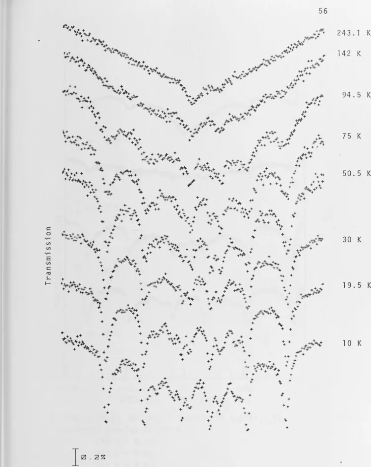
clearly evident from a comparison of the spectra of Figures

(4. l) and (4.2). The spectral behaviour of powdered samples

as the concentration of iron is reduced is discussed 1n the

following paragraph and the spectra are shown in Figure (4.3).

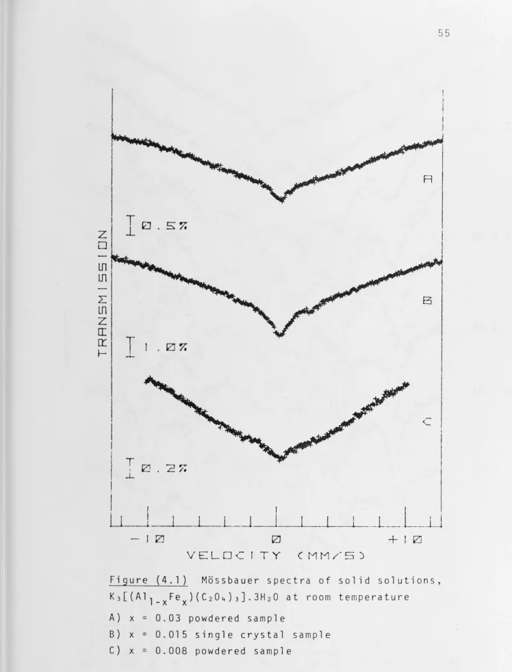
For x = 0.25 the powdered sample yielded a spectrum

showing extensive but incomplete resolution of the hyperfine

structure. The four outer lines are resolved to give broad

peaks but the two inner ones remain obscured by the strong

relaxation-broadened absorption of this complex. When x has

decreased to 0.05 the central absorption had disappeared,

indicating that the Fe(III) ions are sufficiently far apart

for the spin-spin relaxation rate to be long enough to produce

a static hyperfine field at the nucleus (T >>5 x 10- 8 sec).

s

However the spectrum is smeared; six lines are discernible but

they are very broad. At x = 0.03 the lines have sharpened

considerably as a result of a further decrease in the spin-spin

40

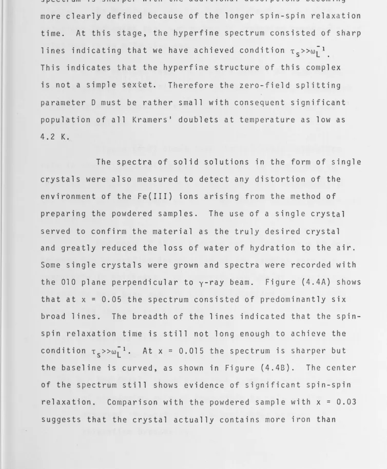
low intensity absorptions have appeared and there are

indications of two more. At higher dilution, x ~ 0.008, the spectrum is sharper with the additional absorptions becoming more clearly defined because of the longer spin-spin relaxati on time. At this stage, the hyperfine spectrum consisted of sharp lines indicating that we have achieved condition Ts>>w~1 .

This indicates that the hyperfine structure of this complex is not a simple sextet~ Therefore the zero-field splitting parameter D must be rather small with consequent significant·

population of all Kramers' doublets at temperature as low as

4.2 K.

The spectra of solid solutions in the form of single crystals were also measured to detect any distortion of the

environment of the Fe(III) ions arising f rom the method of preparing the powdered samples. The use of a single crystal served to confirm the material as the truly desired crystal and greatly reduced the loss of water of hydration to the air .

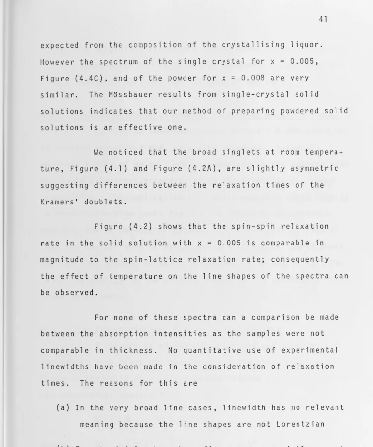
[image:48.787.16.771.194.1108.2]

expected from the composition of the crystallising liquor. However the spectrum of the single crystal for x = 0.005, Figure (4.4C), and of the powder for x = 0.008 are very similar. The M~ssbauer results from single-crystal solid

solutions indicates that our method of preparing powdered solid solutions is an effective one.

We noticed that the broad singlets at room tempera-ture, Figure (4. 1) and Figure (4.2A), are slightly asymmetric suggesting differences between the relaxation times of the Kramers' doublets.

Figure (4.2) shows that the spin-spin relaxation rate in the solid solution with x = 0.005 is comparable in magnitude to the spin-lattice relaxation rate; consequently

the effect of temperature on the line shapes of the spectra can be observed.

For none of these spectra can a comparison be made between the absorption intensities as the samples were not comparable in thickness. No quantitative use of experimental linewidths have been made in the consideration of relaxation times. The reasons for this are

(a) In the very broad line cases, linewidth has no relevant meaning because the line shapes are not Lorentzian

(b) For the fairly sharp hyperfine spectra, variable amounts of broadening make it impossible to rely on the

[image:49.782.15.767.16.1098.2] [image:49.782.9.765.24.929.2]

4.2

42

(c) The unresolved background out of which individual peaks

arise makes it impossible to determine accurately the

width at half maximum for most of the peaks.

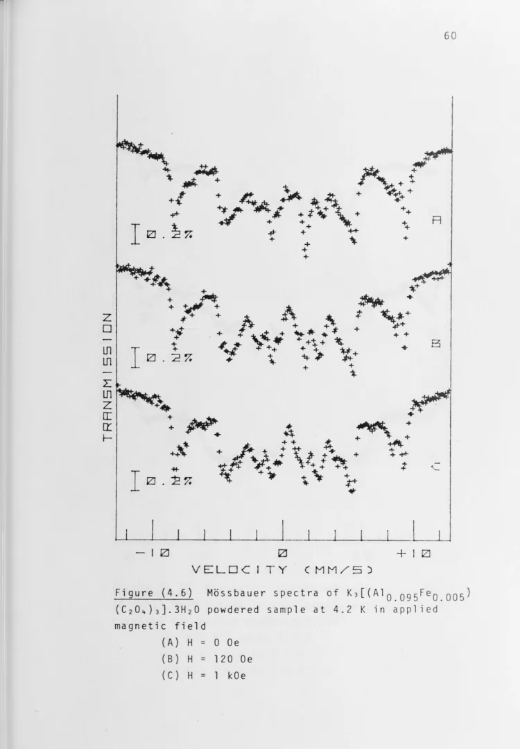
Spectra of powdered samples in applied magnetic fields

Spectra of powdered samples with x = 0.005 and 0.002 ,n applied magnetic fields were also obtained. External

magnetic fields of up to 1 kOe were applied to the samples with

the field direction perpendicular to the direction of y-ray

propagation. The application of a small magnetic field results

in more distinctive peaks for the low intensity absorptions

possibly due to decoupling between electronic spin of Fe(III)

ions and nuclear spin of neighbouring 27

Al nuclei, particularly

for the ±1/2 doublet as shown in Figures (4.5) and (4.6). The better resolution in the central region of the spectra is

immediately seen.

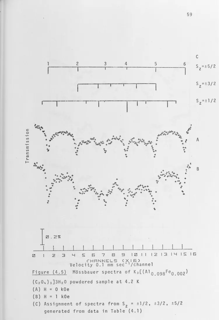
4. 3 The interpretation of experimental spectra

A comparison of calculated spectra and experimental

spectra at zero field has been made and the assignments are

shown in Figure (4.5C). The spin Hamiltonian used in producing

the theoretical spectra is

'J( ₌

'JfC F + 'JfM + J-C _-Q

where _{JCC F} = D{S 2

1

_{~(S +} 1 ) } + E(S 2 -

s

2)

z X y

JCM = A I r, + 1 + S_I+)

2

A(S+I-Z.)Z

J{Q = e

2

9Q 2 _{I ( I + 1 .) + D..( I 2 I:) }}

assuming that EFG tensor and A !1as same principal axes and

coincide with crystal field axes . The unu sually s trong

absorption of line 4, due to overlapping of ±l/2 and ±5/2

transitions, and line 5 due to overlapping of ±3/2 and ±5/2

transitions, destroyed the symmetry of the resol ved hype rfine

spectra. This lack of symmetry increases as the co ncentration

of iron are lowered. This is clearly observed in t he spectra

of solid solutions for various concentrations at 4.2 K,

Figures (4.3) and (4.4).

Comparison of calculated and experimental spectra

yields the following best values for the various paramaters at

4.2 K, table (4. l).

Zero-field splitting parameter D +0.20 + _{0.05 cm-} 1

A = E/ D 0.05 ± _0.01

Asymmetry parameter n* 0. 1 5 + 0.03 _I

Associated hyperfine field

_IHI

540 + 5 k0e or 216 k0e/sp in

Quadrupole interaction energy ¾e2

qQ 0.05 mm sec-1

Table (4.1) Experimentally determined parameters for Fe( I II)

ion in K3[(A1 1_xFex)(C204)3].3H 20 at 4.2 K.

*The parameter n could not be very well determin ed i ndependen tly

as it had little effect on the spectra; n was taken to be equal

to 311.. Much smaller or mu ch -larger values of n gave spectra

44

From the parameters obtained from thi s work, it

1s evident that the site symmetry of Fe(III) ion is not axial

since~: 0.05 and therefore there is some mixing of the

wavefunctions of the Kramers' doublets. The hyperfine field at the Fe(III) nucleus is 540 kOe which is the usual value for an octahedrally-coordinated high-spin Fe(III) complex with

slight covalency effects23 ,72 . The magnitude of quadrupole splitting, ~EQ:o. 10 mm sec- 1 , of this complex rules out the possibility that the Fe(III) oxalate complex intermediate doublet with ~EQ = 0.7 mm sec- 1 arises simply from potassium

trisoxalatoferrate(III) with modified relaxation. The magnitude and sign of the zero-field splitting parameter,

D = +0.20 ± 0.05 cm- 1 (0.29 K) indicates that the S = ±1/2

z

state is the lowest Kramers' doublets, the next ±3/2 and the highest ±5/2. The separation between ±1/2 and ±5/2 states is ::1.2 cm- 1 _{(1.74 K), so that at 4.2 K the three crystal-field}

s t a t e s a re a 1 mo s t e q u a l l y p o p u 1 a t e d ..

4.4 Further investigations

4.4.1 Application of magnetic field to single crystal sample External fields up to 1 kOe were applied to a single crystal sample with x = 0.005; the resulting spectra are shown