Optimal parameters for radiation reaction experiments

This is a repository copy of

Optimal parameters for radiation reaction experiments

.

White Rose Research Online URL for this paper:

http://eprints.whiterose.ac.uk/148408/

Version: Published Version

Article:

Arran, Christopher David, Cole, J. M., Gerstmayr, E. et al. (3 more authors) (2019) Optimal

parameters for radiation reaction experiments. Plasma Physics and Controlled Fusion.

074009. ISSN 1361-6587

https://doi.org/10.1088/1361-6587/ab20f6

eprints@whiterose.ac.uk https://eprints.whiterose.ac.uk/ Reuse

This article is distributed under the terms of the Creative Commons Attribution (CC BY) licence. This licence allows you to distribute, remix, tweak, and build upon the work, even commercially, as long as you credit the authors for the original work. More information and the full terms of the licence here:

https://creativecommons.org/licenses/

Takedown

If you consider content in White Rose Research Online to be in breach of UK law, please notify us by

Plasma Physics and Controlled Fusion

PAPER • OPEN ACCESS

Optimal parameters for radiation reaction experiments

To cite this article: C Arran et al 2019 Plasma Phys. Control. Fusion 61 074009

View the article online for updates and enhancements.

Optimal parameters for radiation reaction

experiments

C Arran

, J M Cole

, E Gerstmayr

, T G Blackburn

,

S P D Mangles

and C P Ridgers

1

York Plasma Institute, University of York, York, United Kingdom

2_{The John Adams Institute for Accelerator Science, Imperial College London, London, United Kingdom} 3

Department of Physics, Chalmers University of Technology, Gothenburg, Sweden

E-mail:christopher.arran@york.ac.uk

Received 25 January 2019, revised 26 April 2019 Accepted for publication 10 May 2019

Published 11 June 2019

Abstract

As new laser facilities are developed with intensities on the scale of1022–1024W cm-2_{, it}

becomes ever more important to understand the effect of strongfield quantum electrodynamic processes, such as quantum radiation reaction, which will play a dominant role in laser-plasma interactions at these intensities. Recent all-optical experiments, where GeV electrons from a laser wakefield accelerator encountered a counter-propagating laser pulse witha0>10, have produced evidence of radiation reaction, but have not conclusively identified quantum effects nor their most suitable theoretical description. Here we show the number of collisions and the conditions required to accomplish this, based on a simulation campaign of radiation reaction experiments under realistic conditions. We conclude that while the critical energy of the photon spectrum distinguishes classical and quantum-corrected models, a better means of distinguishing the stochastic and deterministic quantum models is the change in the electron energy spread. This is robust against shot-to-shotfluctuations and the necessary laser intensity and electron beam energies are already available. For example, we show that so long as the electron energy spread is below 25%, collisions ata0=10 with electron energies of500 MeVcould

differentiate between different quantum models in under 30 shots, even with shot-to-shot variations at the 50% level.

Keywords: radiation reaction, Monte-Carlo simulations, highfield physics, laser-plasma interactions

(Somefigures may appear in colour only in the online journal)

1. Introduction

Experiments using new ultra-high-intensity multi-petawatt laser facilities such as Apollon 10 PW[1]and ELI[2,3]will require a thorough experimental understanding of non-clas-sical behaviour in laser-plasma interactions. In experiments reaching laser intensities of1022–1024W cm-2 _{the effect of}

strongfield QED processes starts to strongly modify the laser-plasma interaction [4–6], and better understanding the

fundamental physical processes at work will be crucial. One of these processes, the radiation produced by charged parti-cles when moving in an electro-magnetic field, and the sub-sequent recoil experienced by the particles, is particularly relevant to studies of inverse Compton scattering [7, 8]and laser absorption in solid target interactions [9–12], both of which are key targets of the ELI-NP facility.

Two recent experiments[13,14]have aimed to study the effect of radiation reaction in isolation, using existing peta-watt laser facilities with peak intensities ofI~1021W cm-2_.

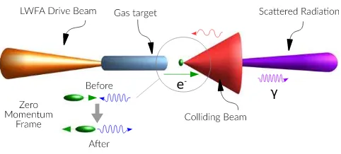
In these all-optical set ups, highly energetic electrons (γ=_1000–2000) produced by a laser wakefield accelerator [15–18] collide with a counter-propagating high intensity laser pulse as shown in the schematic in figure1. In the rest

Plasma Physics and Controlled Fusion

Plasma Phys. Control. Fusion61(2019)074009(11pp) https://doi.org/10.1088/1361-6587/ab20f6

Original content from this work may be used under the terms of the Creative Commons Attribution 3.0 licence. Any further distribution of this work must maintain attribution to the author(s)and the title of the work, journal citation and DOI.

frame of the electron both the frequency and the intensity of the radiation are dramatically increased, bringing the electric field experienced by the electron to the scale of

g

¢ » ~

-EL EL 10 V m17 1, comparable to the Schwinger limit

= ´

-Es 1.32 10 V m18 1 [19], as described by the

dimen-sionless and Lorentz invariant parameterce= ¢EL Es. At this

point the predictions from quantum and classical models of radiation reaction strongly diverge; whereas using the clas-sical synchrotron spectrum requires the production of photons with energiesεγ>εe, the quantum model limits the energy of

photons so as to conserve energy, significantly reducing the synchrotron power at high field strengths, as described in [20–23]. Both of the recent experiments demonstrate sig-nificantly better agreement between their measurements and quantum, non-perturbative, models than with classical models such as described by Landau and Lifshitz[24].

However, the limited number of events measured in the experiments has left significant uncertainty [25], with Poder

et al[14]concluding a slightly better agreement with a semi-classical model, while the measurements made by Coleet al

[13]were not able to distinguish between the semi-classical and stochastic models. In the semi-classical description, both the rate of radiation emission and the subsequent change in electron energy are adjusted to match the quantum model, but the emission remains a continuous process, with the recoil a frictional force that leads to cooler electrons with a narrower energy distribution. In the quantum picture, on the other hand, emission is a quantised, stochastic event; some electrons travel much further through the laser pulse before emitting a photon while others emit many, leading to substantial broadening of the electron energy distribution [26–28]. In modelling stochastic emission events, we assume that photon emission is sufficiently fast that the laser field is constant throughout the process, in the so-called constant-cross-field approximation. This is accurate when the coherence time of emission is much less than the laser period, which generally gives a condition tCOH~mc eEL1 w, for a laser

fre-quencyω[29], or in terms of the normalised vector potential of the laser pulse,a0=eEL mewc1. Even if this

condi-tion is met, however, the constant-crossed-field approx-imation—and both the quantum and semi-classical models—

breaks down when the energy of the emitted photon energy is

very low [30, 31], although these photons do not contribute significantly to the recoil[32].

Experiments currently underway seek to resolve the seeming disparity between the two experiments to date and to determine which, if either, model is most appropriate for high intensity laser experiments; this paper attempts to both find the best way of conducting these radiation reaction experi-ments, and demonstrate the regimes where the choice of model is important. By simulating the experiments under different conditions we place constraints on the parameters required, such as laser intensity and electron energy spread, as well as the accuracy to which these parameters must be controlled. Given different experimental parameters, we estimate the number of measurements required to be confident which model is more appropriate: the stochastic quantum model, or the continuous and deterministic semi-classical model. In doing so, we take account of the shot-to-shot var-iation of both the energy of electrons from a laser wakefield accelerator and the intensity of the colliding laser pulse.

2. Simulated experiments

In a radiation reaction experiment of the type shown in figure1it is important to achieve good overlap in both time and space between the highest intensity region of the laser pulse and the brightest part of the electron beam. However, if the pulse collides with the electron beam close to the LWFA gas target, the electron bunch will be under one micron in diameter. If the collision point is slightly away from the focal plane of the laser, as in[13], it is possible to ensure that the beam profile is much larger than the electron bunch, max-imising the overlap in space and the chances of a successful collision. Under these conditions we can reduce the problem to a single dimension, whereas if this is not the case then accurate knowledge of the transverse electron and laser pro-files at the collision point are required. Similarly, synchrotron radiation is emitted within a forward-pointing cone with an angle of 1/γaround the direction of motion of the electron; for an electron bunch with an angular divergence on the scale of q~1 mrad the total cone angle will be

q g

» +a0 ~10 mrad in the plane of polarisation of the

laser. Under these conditions we will ignore the angular distribution of radiation for energetic electrons. On the short timescale after the creation of the electron beam we can also neglect direct electron–electron interactions such as space-charge, while the electron bunch duration is sufficiently short that we can neglect the interactions of synchrotron photons after they have been emitted. Likewise, as the number of electrons in the bunch is small, we neglect effects of the electron bunch on the laser beam, such as energy loss and refraction. Finally, as we will be considering situations achievable with existing laser facilities, with bothEL/Es=1

and χe  1, we can neglect pair production. We therefore consider the interaction between each electron and the laser pulse independently, allowing us to reduce a complicated simulation to a sum of many single particle interactions, where each electron has a single initial and final energy but

Figure 1.Schematic of an all-optical radiation reaction experiment. An intense ultra-short laser pulse, the LWFA drive beam, is incident upon a gas target, producing a high energy electron bunch. A second intense laser pulse, the colliding beam, is brought to a tight focus just outside the gas target, interacting with the electron bunch and producing a beam of high energy light.

may produce many photons over the course of the interaction with the laser pulse.

First, look-up tables were assembled of thefinal electron and photon spectra resulting when initially mono-energetic electron beams encountered a laser pulse. One dimensional particle-in-cell simulations with EPOCH[33], employing an extended QED module[22](see appendixAfor details), were conducted for laser peak intensities of 1„a0„25 and electron energies of100 ei 2 GeV. These used each in

turn of a fully classical, Landau–Lifshitz, radiation reaction model; a semi-classical model with corrected emission rates and powers but with continuous, deterministic emission; and a quantum model of radiation reaction with stochastic emis-sion. By performing 1D simulations we ignored spatial var-iations in the laser intensity across the electron beam at the collision point. This is valid if the electron beam transverse size is smaller than the laser transverse size at the collision point, as described earlier. The laser pulse had a Gaussian temporal profile with a duration of40 fs FWHM, chosen to reflect parameters of the recent radiation reaction experi-ments. Shorter pulse durations would allow experiments to reach higher laser intensities for the same input energy, reaching higherceµtFWHM

-1

2 _{and exploring more non-classical} effects4. However, in practice, pulse duration is limited by existing laser technology, with shorter pulses typically com-ing at the expense of laser energy.

For each different reaction model, these look-up tables gave final electron and photon energy distributions

e e

( ∣ )

Ne f, f i,a0 and Ng( ∣e eg i,a0). The electron energy

dis-tributions were fitted to a Gaussian to give functions

e e

á ñf ( i,a0) and s eef( i,a0), whereas the photon energy

dis-tributions werefitted to an expression of the form:

e e

e

µ

-g -g g

⎛ ⎝

⎜ ⎞

⎠

⎟ ( )

N exp , 1

crit

2 3

giving the critical energy ecrit(ei,a0). For examples of the

fitted energy distributions, see appendix B. The resulting

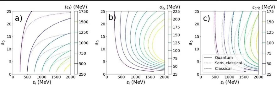
parameters are plotted infigure2using contour plots to show the differences between the three different models.

Firstly, figure 2 demonstrates that the simulations of radiation reaction are working as expected. For a given initial electron energy, increasing the laser intensity reduces thefinal energy of the electrons, while increasing the initial electron energy leads to the emission of higher energy photons. Both of these correspond to a larger radiation reaction force, with an electron beam losing more power, emitted as photons. However, although at low values of a0 the photon critical energy increases with laser intensity, for highera0it saturates and for the highest values of εiactually begins to decrease. This is because electrons lose so much energy during the radiation reaction process that the peak field experienced by the electrons in their rest frame, γEL, is actually reduced. In

this situation the radiated spectrum comprises a greater number of lower energy photons. Similarly, in the quantum model, electrons experience the greatest stochastic broad-ening at moderate laser intensities, around a0≈10, while above this the final energy spread is smaller. At moderate laser intensities electrons emit fewer photons on average, with greater variation between electrons due to shot noise.

The look-up tables also allow us to distinguish between the different models for radiation reaction: as laser intensity increases, the classical model predicts much lower final electron energies than the quantum or semi-classical models. Applying the quantum correction—limiting the photon energy toεγ<εe—results in significantly higherfinal

elec-tron energies and slightly lower photon energies. The greatest difference infinal electron energy occurs at the highest laser intensities and electron energies, whereas the greatest differ-ence in critical energy is centred arounda0≈10.

In both the mean final electron energy and photon energy, it is very difficult to see any difference between the predictions from the quantum and semi-classical models. These models contain the same correction to the power radiated, and on average the electrons encounter the same radiation reaction. However, without the effect of stochastic broadening, an initially mono-energetic electron beam

Figure 2.Contours of(a)the meanfinal electron energyá ñef (b)thefinal electron energy spreadsef and(c)the critical energy of emitted photonsεcrit, for each of the quantum(solid lines), semi-classical(dashed)and classical(dotted)models. Results are from mono-energetic electron beams in EPOCH simulations. Each line shows the initial electron energyεiand the lasera0required to obtain the givenfinal state. For the classical and semi-classical modelssef<1 MeV and hence the contours are not visible.

4

It is possible to show(see appendixC)that forχe=1, reducing the pulse duration for a fixed laser energy only increases the total stochastic broadening, improving the chances of distinguishing between models. For χe0.56, on the other hand, reducing the laser pulse duration is counter-productive.

3

remains mono-energetic in the semi-classical model. In con-trast, in the quantum model the electron energy spectrum becomes substantially broader.

Once the look-up tables á ñe ef ( i,a0), s eef( i,a0) and

ecrit(ei,a0) were assembled, Monte-Carlo simulated experi-ments were conducted for more realistic (though still idea-lised) initial electron energy distributions, which were not mono-energetic, and where each of the laser intensity, the mean electron energy, and the electron energy spread varied shot-to-shot. This allowed us to estimate the underlying three-dimensional probability distribution function f(á ñef ,s eef, crit)

for making measurements of thefinal mean electron energy

á ñEf , and energy spread sEf, and the final photon critical energyεcrit. For parameter scans, the two-dimensional prob-ability distribution functions f₁(á ñef ,ecrit) and f₂(á ñef ,sef) were calculated instead. The details are described in appendixB.

3. Distinguishing models

First, experimental parameters were chosen to match those in [13], with the laser intensity estimated asa0=113and the

electron energy estimated asá ñ =ei (550 20 MeV) , with an

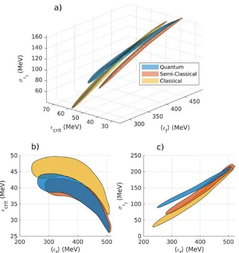
energy spread of sei=250 MeV. The three-dimensional dis-tribution functions, shown in figure 3, demonstrate the cap-ability of the simulated experiments. Points in the top right of the image correspond to shots with low a0, with high final energies, high energy spread, and lower photon energies. In this regime, the three models predict very similar results. As a0 increases, the electron beam loses more energy and becomes cooler with a lower energy spread, in the process producing higher energy photons. At the largest values ofa0, the different rates of radiation reaction and of radiative cooling lead to the three models predicting different results, with the classical model leading to the lowestfinal energy spread and the highest photon energy, while the quantum model predicts a sig-nificantly higher energy spread than either of the two other models. The shot-to-shot variation ofá ñei tends to blur out this

trend, broadening the distribution functions and making it more difficult to distinguish between different models.

In order to show this more clearly, and to compare the results with [13], the two-dimensional distribution functions

f1 and f2 were calculated for laser intensities pulled from a uniform distribution between a0=4 and a0=20.

e e

á ñ

( )

f₁ f , crit , shown in figure 3(b), agrees well with the

previous work, with the classical model predicting sub-stantially higher critical energies as expected. The predictions from the quantum and semi-classical models strongly overlap, however, and hence using critical energy from the photon spectra is a poor way of determining between stochastic and semi-classical models of radiation reaction.

Figure 3(c), however, shows another possible measure-ment using the same experimeasure-mental parameters, comparing the mean final electron energy with the final energy spread, as described by f₂(á ñef ,sef). Using these measurements the semi-classical and classical models predict fairly similar results, but the quantum model predicts a substantially higher energy spread than both of the other models. This is because, for an interaction where the electron beam is much smaller than the focal spot, these deterministic models predict that electron beams can only ever become cooled by emitting synchrotron radiation in the electricfield of the laser, as more energetic electrons emit radiation more strongly. In the sto-chastic model, however, the number and energy of photons emitted by each electron is probabilistic and varies strongly. In certain cases, the final energy spread of the electron may increase over time(see for instance [27,28,34]). The lower the energy spread, the more likely this becomes. Reference [27]equation(3.8)predicts that for Gaussian energy spectra the cross-over point, below which the stochastic broadening dominates, can be approximated in the caseseiá ñei by:

s

e c

á ñ » á ñ

e ⎛

⎝ ⎜ ⎞

⎠ ⎟

· ( )

55 3

8 24 , 2

i

e

2 i

s

e c

á ñ » á ñ

e

( )

0.70 . 3

i

e

i

We can quantify the ease of distinguishing between models by measuring the overlap between the joint dis-tribution functions. The probability of making a measure-ment of several parameters, denoted by the vector x_{, given}

Figure 3.Results from simulated radiation reaction experiments for an initial electron beam with a peak energy of(55020 MeV) and an energy spread of250 MeV, shown through(a)the three-dimensional joint probability distribution function f(á ñef ,ecrit,sef), and the 2D distribution functions(b) f₁(á ñef ,ecrit)and

(c) f2(á ñef ,s_ef). The 1σcontours are shown, within which 68% of simulated experiments measured these results, assuming each of the classical(yellow), semi-classical(red), and quantum(blue)models. In(a)the intensity of the colliding laser pulse isa0=11±3, whereas for(b)and(c)the intensity was assumed uniformly distributed betweena0=4–20, for comparison withfigure 9 of[13].

that a model A is true, is denoted P( ∣ )xA . The chances of incorrectly inferring modelBfrom those measurements can be related by Bayes’ theorem to the model probability as

=

( ∣ ) ( ∣ ) ( ) ( )

P Bx P xB P B P x. If the prior assumption is that the two models are equally likely, but not the only two possible models, and that all measurements ofx_{in the region} of interest are equally likely, with no bias in the measuring equipment, we can show that the probability of incorrectly inferring modelBfrom a single measurement ofx_{, if model}

A is true (or vice versa) is proportional to the overlap Ω

between the models, as:

ò

ò

ò

= = W º

( ∣ ) ( ∣ ) ( ∣ ) · ( ∣ )

( ∣ ) ( ∣ )

( )

P B A P A B P A P B V

P A V P B V

x x x x d d d , 4 x x x 2 2

where the integrations are performed over the domain of possible measurements within whichP(x_{)is constant. This} probability is normalised such that ifP( ∣ )xA =P( ∣ )xB then

Ω=_{1. Depending on the choice of measurements,} P( ∣ )xA andP( ∣ )xB are described by the joint distribution functions

e e

á ñ

( )

f₁ f , crit and f₂(á ñef ,sef)for each model.

If N independent and identically distributed measure-ments are taken, one for each successful laser-beam collision, the probability of incorrectly inferring modelB, given thatA

is in fact true, becomes P B A( ∣ )= WN_{. Conversely, if we}

require better than a certain degree of accuracy to be sure we will not incorrectly infer model B, such that P B A( ∣ )<p, we can show that we requireN>logp logW. If the overlap between the joint distribution functions is very high,W 1,

W 

∣log ∣ 0 and it becomes increasingly difficult to confirm which model is correct, requiring an ever larger number of shots.

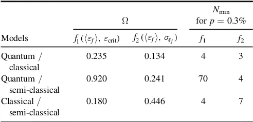
This is shown in table1for the parameters described in [13]and joint distribution functions shown in figure 3. The classical model predicts significantly different results to the quantum and semi-classical models and hence the overlap and number of shots required are both small. The work in [13] was therefore able to show that the quantum model agreed better with the data than the classical model, despite only definitely measuring four successful collisions. In general, measurements ofεcritandá ñef are successful at determining

between classical and quantum/semi-classical models of radiation reaction. With those measurements, however, it would be more difficult to distinguish between the quantum and semi-classical models, with at least 70 shots required to obtain the same level of certainty.

An alternative approach is to measuresef, therefore sig-nificantly reducing both the overlap between the models and the number of shots required. Although an accurate mea-surement ofsef is difficult, requiring a clean electron energy spectrum, the difference in the predictions from quantum and semi-classical models is significant. For certain experimental parameters, using this measurement could reduce by more than an order of magnitude the number of shots required to confidently determine which model is more appropriate.

4. Optimal parameters

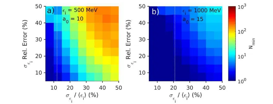
The overlap between the joint distribution functions assuming quantum and semi-classical models of radiation reaction was tabulated over a wide range of different initial electron energies and laser intensities in order to determine the number of shots required to distinguish at thep=_{0.3% level between} the two models given certain experimental parameters. Similar values as before for the uncertainties in a0 andá ñei

were used, at±_{3% and}±_{10% respectively, with a very large} energy spread of sei á ñ =ei 50% as before. In order to

describe realistic experiments, shot-to-shot variation onseihas also been introduced, at ±_{25% of} s_{ei, such that the laser} intensity, mean electron energy, and electron energy spread all vary shot-to-shot. The results are shown infigure4.

Figure 4(a) shows the number of shots required when using measurements ofá ñef and εcrit; this demonstrates that

when operating at realistic experimental parameters, many shots must be taken to distinguish between quantum and semi-classical models of radiation reaction. For low a0and

e

á ñi, hundreds of shots are required to conclude that one of the

models is correct and not the other. In contrast to the situation for mono-energetic electron beams, increasing the laser intensity abovea0=10 increases the difference between the predictions from the two models. If it is possible to increase the electron energy toá ñei 1 GeVand the laser intensity to a0…15, the number of shots required is reduced to below 25. Under these conditions, a practical radiation reaction experi-ment could determine with significant (>_3σ) confidence which model is more appropriate in this regime.

If we cannot determine between quantum and semi-classical models of radiation reaction using measurements of

e

á ñf and εcrit, it is possible to use a measurement of the final

electron energy spreadsef. As shown infigure4(b), this does not reduce the number of shots required at low laser inten-sities, but is substantially more successful at lower electron energies, with fewer than 25 shots required ifá ñei 500 MeV

anda0…15. For sufficiently high electron energies and laser intensities (for instanceá ñei 1 GeV and a0…20, the pre-dictions from the quantum and semi-classical models for radiation reaction are substantially different; under these conditions, it is vital to understand which model of radiation

Table 1.OverlapΩof joint distribution functionsf1andf2and corresponding minimum number of shots required to obtain 3σ confidence in determining between models for radiation reaction, using different sets of measurements.

Ω

Nmin forp=0.3%

Models f1(á ñef ,ecrit) f₂(á ñef ,sef) f1 f2 Quantum/

classical

0.235 0.134 4 3

Quantum/

semi-classical

0.920 0.241 70 4

Classical/

semi-classical

0.180 0.446 4 7

5

reaction is more accurate, and only a single shot may be sufficient to discriminate between quantum and semi-classical models.

It is clear that the energy spread of the electron spectrum is the key distinguishing feature of a stochastic model as opposed to a deterministic model, and we can study the effect of decreasing the initial energy spread in the electron spec-trum. This will reduce the cooling experienced by the electron beam, increasing the relative contribution of stochasticity. Simulated experiments were run as before, but with the relative energy spread reduced to 20% and 10%. Again, the relative variation of the energy spread was±25%, giving energy spreads of sei=(0.20.05)á ñei and

e

 á ñ

(0.1 0.025) i, respectively. As shown in figure 5,

redu-cing the initial energy spread significantly changes the final energy spread and reduces the number of shots required to determine which model is more suitable. If no more than one hundred shots are possible and the relative energy spread is 20%, distinguishing between the models requires just



e

á ñi 500 MeV or a0…12. Under most conditions simu-lated, fewer than 10 shots would be required. For an energy

spread of 10%, however, the models can easily be dis-tinguished even for the lowest laser intensities and electron energies. Only atá ñ =ei 200 MeVanda0=5 do the models predict very similar outcomes; under these conditions the accuracy of the constant-cross-field approximation is doubtful and it is likely that both models will break down. In most of the simulated experiments, however, only a single shot would be sufficient to determine which model is more correct. Reducing the energy spread of the initial electron beam is therefore one of the best ways of ensuring an experiment will be able to distinguish between deterministic and stochastic models of radiation reaction.

We can study the maximum allowable energy spread at a certain laser intensity and initial electron energy, if stochastic effects are to be measured. First, we ran simulated experiments for a0=10±3 andá ñ =ei (500 50 MeV) , which

corre-sponds to a quantum parameter á ñ = ác_e g_eE EL sñ »0.03.

These parameters are achievable in many existing PW scale laser facilities, and are on the same scale as achieved previously in[13]. The results, plotted infigure6(a), show the number of shots required for a range of energy spreadsseiand errors on the

Figure 4.The estimated number of shots required to distinguish between the quantum and semi-classical models at thep=0.3%significance level using measurement of(a)á ñef andεcritand(b)á ñef andsef, plotted against the laser intensitya0and the electron energyεi. The variation

ona0was taken to be±3, and the shot-to-shot variation oná ñei was±10%. The initial energy spread wassei=(0.50.125)á ñei. The colour

scale is the same for both plots.

Figure 5.Using an initial energy spread of(a)sei á ñ =ei 20%5%and(b)sei á ñ =ei 10%2.5%, the estimated number of shots required

to distinguish between quantum and semi-classical models of radiation reaction at a confidence level ofp=0.3%. All values are using

measurements ofá ñef andsef and are plotted against the laser intensitya0and the electron energyεi. The shot-to-shot variation ona0was taken to be±3, and the variation ofεiwas±10%. The colour scale is the same for both plots.

energy spread. The number of shots required increases with both the energy spread and the variation in the energy spread, and is sufficient to make experiments impractical when either of these are high. For an experiment to be practical, requiring only 10s of shots to successfully distinguish between models, the energy spread must generally be kept below around



sei á ñei 25%. If the relative error on the energy spread can

be greatly reduced, however, experiments with these parameters can be successful whilesei á ñei 50%. For á ñ »ce 0.03 in

equation(3), the energy spread required for the electron spec-trum to broaden is sei á ñei 12%, below which simulated

experiments measure a clear difference between quantum and semi-classical models. However, the simulated experiments show that a significant difference arises between the two models well before stochastic broadening dominates, so long as the variation on the energy spread is limited to a few tens of percent or lower.

We also ran simulated experiments fora0=15±3 and

e

á ñ =i (1.00.1 GeV) , orá ñ »ce 0.1, parameters which are

around the limit of what is achievable with some of the existing petawatt laser facilities(e.g.[14]). Figure6(b)shows the results, demonstrating that the number of shots required is greatly reduced at these parameters. Under these conditions, it is relatively straightforward to distinguish between the quantum and semi-classical models, with the predicted energy spread significantly different even when the energy spread is on the level ofsei á ñ »ei 50%and varies widely shot-to-shot.

Again, we can calculate where stochastic broadening dom-inates analytically using equation (3), giving a condition on the energy spread ofsei á ñei 20%. With this increased laser

intensity and electron energy, the simulations show that the predictions of the two models diverge even well above this threshold, with the stochastic model predicting a large reduction in the cooling rate and a significantly differentfinal energy spread.

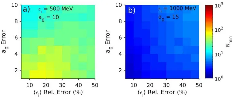
Finally, we explored the effect of shot-to-shot variation of the laser intensity and mean initial electron energy under the same two sets of conditions: a0=10 and

e

á ñ =i 500 MeV;anda0=15 andá ñ =ei 1 GeV. The energy

spread was set assei=0.25á ñei, with the shot-to-shot

varia-tion on the energy spread0.25sei. Figure7shows the number of shots required at a range of errors on both a0 and á ñei.

Interestingly, the effect is small, with no drastic change in the overlap between predictions from the two different models. At a higher laser intensity and electron energy the number of shots required increases slowly with an increasing shot-to-shot variation, as expected. At the lower intensity and electron energy, however, large variation actually results in more significant radiation reaction effects in the high energy and high intensity tails, causing a slight reduction in the number of shots required. Experiments will remain able to distinguish between stochastic and deterministic models of radiation reaction even if the shot-to-shot variation in the laser intensity and electron energy are high, so long as the shot-to-shot variation in electron energy spread is limited.

In the course of these simulated experiments we have considered a wide range of experimental errors, but the laser pulse profile and the electron energy distribution have remained idealised. In practice, electron bunches from LWFA often contain a significant lower energy or thermal comp-onent, particularly when operating in the so-called ‘bubble’

regime [35], where electrons are continuously injected into the wakefield. This work has neglected that background, which would have to be carefully removed from the energy spectrum before measuring the final energy spread of the beam. Spatial variation in both the electron beam and the laser pulse can also result in significant changes to thefinal electron energy spread; if one region of the electron beam experiences a much higher laser intensity and a greater radiation reaction force, thefinal energy spread of the beam can be significantly higher than expected. Practical experiments must work to limit the spatial variation, which can be achieved by moving the focal plane of the laser pulse further away from the point of collision with the electron beam, at the cost of reducing the effective laser intensity. Future simulated experiments, on the

Figure 6.Using initial conditions of(a)a0=10±3 andá ñ =ei (50050 MeV) , and(b)a0=15±3 andá ñ =ei (1.00.1 GeV) , the

number of shots required for Monte-Carlo simulated experiments to determine with 3σconfidence between the quantum and semi-classical models. All values are using measurements ofá ñef andsef and are plotted against the electron energy spread, relative to the mean electron energy, and the shot-to-shot variation of the electron energy spread, relative to the energy spread. The colour scale is the same for both plots. The analytic prediction to measure stochastic broadening in the ideal case is also shown(white dotted line).

7

other hand, could include variation of the laser intensity within a single shot, as well as shot-to-shot[36].

5. Conclusions

We have used a series of particle-in-cell simulations and Monte-Carlo simulated experiments to make predictions for radiation reaction from each of the quantum, classical, and semi-classical models using realistic parameters. In doing so, we have shown that while measurements correlating the cri-tical energy of the resulting photon spectra with the mean final electron energy give a way of clearly distinguishing the classical model from the quantum and semi-classical models, this is a poor way of determining which of the quantum and semi-classical models to use. For laser intensitiesa0<15 and electron energies ei<1 GeV, these two models predict

almost the samefinal average energy of electrons and pho-tons, for both mono-energetic electron beams and more rea-listic broad electron distributions.

Instead, we have shown that measuring the energy spread of the electron spectrum after the interaction gives a clearer distinction between the stochastic and deterministic models. Although the energy spread will only increase over the course of the interaction when the initial energy spread is very low (aroundsei á ñei 12%fora0=10 andei=500 MeV), the

effect of stochasticity substantially reduces the rate of cool-ing, leading to different predictions from the quantum and semi-classical models even at much higher energy spreads.

We have used the simulated experiments to determine how many shots would be required when operating at certain conditions, and used this to build up a picture of the optimal experimental parameters. Crucially electron energy spread should be reduced to below 25%, if possible, to maximise the chances of conclusively determining which model is more accurate, while shot-to-shot variation on the energy spread should be minimised. At this energy spread, it should be possible to distinguish the quantum and semi-classical models in a few shots even with relatively unambitious experimental

parameters, such as á ñ =ei 500 MeV and a0=10. Under these conditions, the measurement is robust to significant shot-to-shot variation in electron energy and laser intensity, even on the scale of 50%.

Alternatively, if it is difficult to reduce the electron energy spread, increasing the electron energy or laser inten-sity will separate the predictions from the two models. Even with an energy spread ofsei=50%, it is possible to distin-guish between the models fairly clearly if a0>10 and

e

á ñ >i 1 GeV, or if a0>15 and á ñ >ei 500 MeV. By an

electron energy of á ñ =ei 1 GeV and a laser intensity of a0=15, the models can be fairly easily distinguished regardless of a large energy spread or shot-to-shot variation. These requirements are certainly achievable using current laser systems, and upcoming experiments should be able to clearly determine which model of radiation reaction is most suitable for describing interactions of energetic electrons with high intensity lasers.

Acknowledgments

CA and CPR are grateful for EPSRC Grant No. EP/ M018156/1 which made this work possible. This project has received funding from the European Research Council(ERC) under the European Union’s Horizon 2020 research and innovation programme(Grant Agreement No. 682399), from EPSRC Grant No. EP/M018555/1, and from the Knut and Alice Wallenberg Foundation. Simulations used the EPOCH PIC code developed under UK EPSRC Grants EP/G054950/ 1, EP/G056803/1, EP/G055165/1 and EP/ M022463/1, while computing resources were provided by STFC Scientific Computing Department’s SCARF cluster.

Appendix A. EPOCH revisions

The quantum electro-dynamics model in EPOCH described in detail in[22]is a Monte-Carlo stochastic model which takes

Figure 7.For(a)a0=10 andá ñ =ei 500 MeV, and(b)a0=15 andá ñ =ei 1 GeV, the estimated number of shots required to distinguish at

thep=0.3% signi_ficance level between the quantum and semi-classical models. All values are using measurements ofá ñef andsef and are plotted against the relative shot-to-shot variation on the initial electron energy and the variation on the laser intensity. The colour scale is the same for both plots.

into account both the changes to the synchrotron spectrum and emission rate as the effective electricfield rises, and also the random nature of the photon emissions. A charged macro-particle is initialised with a random optical depth τ0. Its optical depth is then reduced at every timestep by:

t =t- - Ng ·d ( )

t t

d

d , A1

n n 1

wheretn is the optical depth at thenth timestep andδtis the

duration of the timestep. When the optical depth falls below zero, the macro-particle emits a single macro-photon, with a particle weight equal to that of the original macro-particle and an energy chosen at random from the relevant synchrotron spectrum, as:

e g c

c

=

g 2m ce e g, (A2)

e

2

=

g ( )

w we, A3

where χγ is chosen from the synchrotron spectrum c c

cg( g∣ )

P e, wherece=geE EL s, wherege= +1 ee m ce 2 is

the usual relativistic factor, and Es»1.32´10 V m18 -1 is

the Schwinger limit.

We wish, however, to explore two alternative determi-nistic models: the fully classical model, which possesses neither the random nature of emission nor the changes to the synchrotron spectrum and emission rate; and the so-called semi-classical model, which contains the changes to the synchrotron spectrum and rate, but not the random emission. In these two models, each electron now emits a macro-photon at every timestep, ignoring the optical depth. The energy is chosen at random from the relevant synchrotron spectrum as before(with the classical model using the limit of the synchrotron spectrum asce0), but the particle weight

of this macro-photon is now proportional to the instantaneous emission rate and the timestep duration as:

d

=

g · g · ( )

w w N

t t

d

d A4

e

In this way, the semi-classical model will predict the same photon energy spectrum and rate of emission as the quantum model, but the semi-classical model is deterministic, with no element of randomness. In this model, charged par-ticles continually emit photons.

For vanishing smallEL0both the particle weight and

energy of the macro-photon should vanish to zero and emission under these conditions will contribute negligibly to

the final photon spectrum. There is, however, an additional

complexity due to the implementation of P_cg(c c_g∣ e) in EPOCH. This is tabulated, and has a lower limit asχe van-ishes to zero withEL0, at a valuece,min. This implies that

asχevanishes to zero,χγdoes not, and soeg  ¥, which is

clearly unphysical.

Asc_e0,Pcg(c cg∣ e) should instead tend towards the

classical limit, where the synchrotron spectrum is a function of a single variable only: Pcg(c cg∣ e)P(c cg e)

2 _{. For}

ce<ce,min, we instead calculate the photon energy using:

c c c

c = ¢ g g ⎛ ⎝ ⎜⎜ ⎞ ⎠

⎟⎟ , (A5)

e

e,min 2

where c¢_g is chosen at random from Pcg(c c_g¢∣ e,min). In this

way, even though c¢_g cannot vanish to zero, both χγ and eg µc cg ewill safely vanish to zero asce0.

This step is not generally necessary in the stochastic case, as the probability of emitting a macro-photon vanishes to zero as EL0, so photons with un-physically high energies are

never created. When emitting a macro-photon at every timestep, however, this step is important to avoid a large population of extremely high energy macro-photons, even though the particle weights of these macro-photons safely vanish to zero.

Appendix B. Monte-Carlo simulated experiments

For each simulated shot, values for the laser intensity, para-meterised bya₀( )n, the mean initial electron energyá ñe ( )

i n, and the

initial energy spreads_e( )n_i were randomly chosen from Gaussian distributions with a chosen mean and standard deviation.

Nelectron=10 000 electrons were then simulated, each with an initial energye( )i

s

sampled from another Gaussian distribution, with meaná ñe ( )

i n and standard deviations( )eni . For each simulated electron, the final energy distribution was characterised by a Gaussian with mean á ñe ef ( ( )is,a0( )n) and standard deviation

s ee( ( )i ,a( ))

s n

0

f drawn from the look-up table, and thefinal elec-tron energy was then estimated by drawing a random samplee( ) f

s

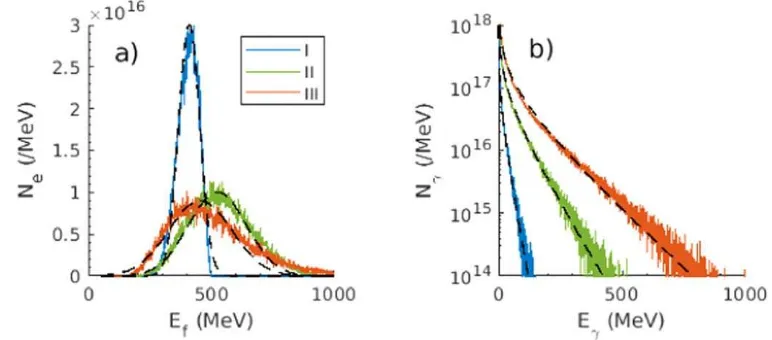
from this distribution. Example electron energy spectra from the mono-energetic simulations are shown infigureB1(a)alongside the Gaussianfits. When the electron energy and laser intensity are very high, thefinal electron spectra are strongly skewed and the Gaussian distribution becomes a worse approximation, but at the laser intensities and electron energies considered in this paper the divergence is small.

A histogram was assembled for each shot, using the

Nelectrondifferent values ofe( )f s

, and this wasfitted to a Gaussian to estimateá ñe ( )

f n ands_e( )n_f . At the same time, for each electron

the photon distribution Ng( ∣e eg ( )i ,a( ))

s n

0 was calculated from

the look-up table and added to a total distribution

e

g( )( ∣g ( ) ( )) Nn Ne i,a

n n

, 0 . This was thenfitted to equation(1)to give

an estimatee( )_critn . Examples of photon spectra from the mono-energetic simulations are shown infigureB1(b)alongsidefits to equation(1). Summing the photon spectra means that, as in real experiments, the much higher number of photons emitted by the highest energy electrons tend to dominate the spectrum and using e( )n

crit remains a reasonable way of parameterising the

measured spectrum.

In total, Nshots=10 000 shots were simulated, and the different estimates of á ñe ( )

f n, s_e( )n_f and e( )_critn were combined

using a Gaussian kernel-density estimate to form the joint distribution function f(ecrit,á ñef ,sef). The process was repeated for each of the classical, semi-classical and quantum models of radiation reaction, using the appropriate look-up tables, giving three different joint distribution functionsf(Q),

9

f(S), and f(C). For parameter scans, however, it is computa-tionally expensive to calculate the three-dimensional dis-tribution function, and so the two-dimensional disdis-tribution functions f1(á ñef ,ecrit)and f2(á ñef ,sef)were used. These are effectively integrations of f(ecrit,á ñef ,sef), integrated over

sef orεcritrespectively, and require justNshots=1000 shots to accurately sample the underlying distribution. Convergence testing, varyingNshots, allowed us to estimate the error on the probability under these conditions as approximately 5%.

Appendix C. Optimal pulse duration

In order to study the optimal pulse duration we can consider the stochastic contribution to broadening of the electron energy distribution. This is described by the second moment of the synchrotron emission distribution function(or thefirst moment of the synchrotron energy spectrum)[27]:

ò

ò

c c c c c

c c c c

º

c

g g g

g g g

¥ ( ) ( ) ( ) ( ) g F F , d

4 3 d , C1

e e e 2 0 2 0 cl 2 e

where F(χe, χγ) and Fcl(4c_g 3ce2) are the quantum

and classical synchrotron functions respectively, which describe the energy spectra [21]. The function g2(ce) can be approximated by g2(ce)»[1 +(1 +4.528ce)

c

+

( )

ln 1 12.29 e + 4.632ce]

-2 7 6_.

Stochastic broadening results in a rate of increase in the variances2º á ñ - á ñg2 g 2_{, described by:}

s ₌ á ñ

+ ⎛ ⎝ ⎜ ⎞ ⎠ ⎟ ( ) t S m c d

d e , C2

2

2 4

where

c a

t gc c

=

( )

¯ ( ) ( )

S 55 m c g

24 3 , C3

e

c

e2 4 e3 2 e

and the averageá ñS is taken over the electron population. For a laser pulse with a durationτ and a total energy E,

c µg_a µg t_E

-e 0

1 2

1

2and the total increase in the energy spread due to this stochastic emission is therefore described by:

s gc c t

g c c

D µ µ

( )

( ) ( )

g

E g . C4

e e e e 2 3 2 3 2

At lowχe=1,g₂(c_e)»1, and for afixed laser energy, broadening only increases as the pulse duration falls, as

s g t

D 2µ_E3 4 -2

1

2. However, forχ_e?1,g2(ce)falls towards zero asg2(ce)µc-e

7

3 and the increase in energy spread also

falls towards zero asDs2µEg c3 -_e43µE13g t 5 3

2 3.

The increase in energy spread is maximal in between these two regimes, where:

s

c c c

c c ¶D ¶ = = + ¶ ¶ ( ) ( ) ( ) g g

0 . C5

e e e e e 2 2 2

Solving this numerically gives χe≈0.56, which for a

»2 GeV electron bunch corresponds to a0≈50. This is beyond the regime explored by the radiation reaction experi-ments considered in this paper, but well within the capabilities of 10 PW laser facilities. The results of this paper, considering onlya0„25, suggest increasing the laser intensity in order to better distinguish between models of radiation reaction, but experiments using 10 PW laser facilities could consider using laser pulses which are not fully compressed, with lower inten-sities than the maximum possible laser intensity, in order to increase the broadening of the electron energy distribution in future radiation reaction experiments.

ORCID iDs

C Arran https://orcid.org/0000-0002-8644-8118

E Gerstmayr https://orcid.org/0000-0003-1164-8593

T G Blackburn https://orcid.org/0000-0002-3681-356X

References

[1] Zou Jet al2015High Power Laser Sci. Eng.3₂ [2] Weber Set al2017Matter Radiat. Extremes2₁₄₉

Figure B1.Example spectra for(a)electrons and(b)photons resulting from simulations of mono-energetic electron beams interacting with laser pulses. Electron spectra werefitted to Gaussian distributions(dashed black lines), whereas photon spectra werefitted to equation(1). Conditions were(I)a low laser intensity and electron energy(a0=10,Ei=500 MeV,(II)a moderate intensity and energy(a0=15,

=

Ei 1000 MeV), and(III)a high intensity and energy(a0=20,Ei=1500 MeV).

[3] Gales Set al2018Rep. Prog. Phys.81₀₉₄₃₀₁

[4] Bell A R and Kirk J G 2008Phys. Rev. Lett.101₂₀₀₄₀₃ [5] Di Piazza A, Müller C, Hatsagortsyan K Z and Keitel C H

2012Rev. Mod. Phys.84₁₁₇₇

[6] Mourou G A, Tajima T and Bulanov S V 2006Rev. Mod. Phys.78₃₀₉

[7] Powers N D, Ghebregziabher I, Golovin G, Liu C, Chen S, Banerjee S, Zhang J and Umstadter D P 2013Nat. Photon.

8₂₈

[8] Tsai H Eet al2016Phys. Plasmas22₀₂₃₁₀₆

[9] Duff M J, Capdessus R, Sorbo D D, Ridgers C P, King M and McKenna P 2018Plasma Phys. Control. Fusion60 064006

[10] Tamburini M, Pegoraro F, Piazza A D, Keitel C H and Macchi A 2010New J. Phys.12₁₂₃₀₀₅

[11] Zhang P, Ridgers C P and Thomas A G R 2015New J. Phys.

17₀₄₃₀₅₁

[12] Wang W-M, Gibbon P, Sheng Z-M, Li Y-T and Zhang J 2017

Phys. Rev.E96₀₁₃₂₀₁

[13] Cole J Met al2018Phys. Rev.X8₀₁₁₀₂₀ [14] Poder Ket al2018Phys. Rev.X8₀₃₁₀₀₄

[15] Tajima T and Dawson J 1979Phys. Rev. Lett.43₂₆₇ [16] Mangles S P D, Murphy C D and Najmudin Z 2004Nature

431₅₃₅

[17] Faure J, Glinec Y, Pukhov A, Kiselev S, Gordienko S, Lefebvre E, Rousseau J-P, Burgy F and Malka V 2004

Nature431₅₄₁

[18] Geddes C G R, Toth C S, Van Tilborg J, Esarey E, Schroeder C B, Bruhwiler D, Nieter C, Cary J and Leemans W P 2004Nature431₅₃₈

[19] Schwinger J 1951Phys. Rev.82₆₆₄ [20] Erber T 1966Rev. Mod. Phys.38₆₂₆

[21] Sokolov I V, Nees J A, Yanovsky V P, Naumova N M and Mourou G A 2010Phys. Rev.E81₀₃₆₄₁₂

[22] Ridgers C, Kirk J, Duclous R, Blackburn T, Brady C, Bennett K, Arber T and Bell A 2014J. Comput. Phys.260₂₇₃ [23] Blackburn T G, Ridgers C P, Kirk J G and Bell A R 2014Phys.

Rev. Lett.112₀₁₅₀₀₁

[24] Landau L D and Lifshitz E M 1971The Classical Theory of Fields, vol 2 3rd edn(Oxford: Pergamon)

[25] Macchi A 2018APS Phys.11₁₃

[26] Neitz N and Piazza A Di 2013Phys. Rev. Lett.111₀₅₄₈₀₂ [27] Ridgers C Pet al2017J. Plasma Phys.83_715830502 [28] Niel F, Riconda C, Amiranoff F, Duclous R and Grech M 2018

Phys. Rev.E97₀₄₃₂₀₉

[29] Ritus V I 1985J. Russ. Laser Res.6₄₉₇

[30] Harvey C N, Ilderton A and King B 2015Phys. Rev.A91 013822

[31] Di Piazza A, Tamburini M, Meuren S and Keitel C H 2018

Phys. Rev.A98₀₁₂₁₃₄

[32] Blackburn T G, Seipt D, Bulanov S S and Marklund M 2018

Phys. Plasmas25₀₈₃₁₀₈

[33] Arber T Det al2015Plasma Phys. Control. Fusion57₁₁₃₀₀₁ [34] Vranic M, Grismayer T, Fonseca R A and Silva L O 2016New

J. Phys.18₀₇₃₀₃₅

[35] Pukhov A M, Gordienko S, Kiselev S and Kostyukov I 2004

Plasma Phys. Control. Fusion46_B179

[36] Baird C D, Murphy C D, Blackburn T G, Ilderton A, Mangles S P D, Marklund M and Ridgers C P 2019New J. Phys21₀₅₃₀₃₀

11