Is the EU internal market suffering from an integration deficit? Estimating the 'home bias effect ' CEPS Working Document No 348, May 2011

Is the EU internal market suffering

from an integration deficit?

Estimating the ‘home-bias effect’

Consuelo Pacchioli*

No. 348, May 2011

Abstract

As an alternative to measuring the extent of market integration, ‘home-bias’ indicates the degree to which economic agents ‘over-prefer’ to transact with domestic agents rather than agents from other EU countries. Such an exclusive preference is measured against a benchmark of (ideal) market integration and is called ‘home-bias’.

This CEPS Working Document addresses the estimation of a ‘normal trade’ gravity equation to establish the possible existence of home-bias effects in the US market and the EU internal market, which are the two most integrated regions in the world. Estimations based on pooled OLS cross-section analysis, with the novelty of the inclusion of time dummies in order to obtain unique indexes and panel data-fixed effects, both reject the hypothesis of no internal barrier to trade. This shows a tendency to ‘over-trade’ within borders both in the US and the EU. Taking the finding for the US market as a benchmark, a direct comparison with the EU internal market is considered: the estimated results show that an average EU country still trades more within its borders than with other member states – about three to four times as much as a random US state does. A number of explanations are offered for this relatively low level of EU internal market integration.

Key words: Borders, European Union, market integration, gravity, economic integration JEL codes: F15, O52

* Consuelo Pacchioli ([email protected]) was a researcher at CEPS at the time of writing this paper. The author is most grateful to Professor Jacques Pelkmans for his guidance, his detailed and constructive comments, and his invaluable support throughout the work.

CEPS Working Documents are intended to give an indication of work being conducted within CEPS research programmes and to stimulate reactions from other experts in the field. Unless otherwise indicated, the views expressed are attributable only to the authors in a personal capacity and not to any institution with which they are associated.

ISBN 978-94-6138-092-0

Introduction ... 1 

1.  Literature review ... 2 

1.1  Early empirical evidence ... 2 

1.2  The theory ... 5 

2.  The empirical model: estimation techniques and data ... 6 

2.1  Comparing US and EU internal markets ... 6 

2.1.1  Analysis of the data: the US market ... 10 

2.1.2  Analysis of the data: the EU market ... 11 

2.2  US versus EU internal market: empirical model ... 12 

3.  Presentation of the results and assessments ... 13 

3.1  Empirical estimates ... 13 

3.2  Possible interpretations of the results ... 15 

4.  Conclusions ... 17 

References ... 18 

Annex ... 20 

|1

Estimating the ‘home-bias effect’

CEPS Working Document No. 348 / May 2011

Consuelo Pacchioli

Introduction

As acknowledged by the most widely recognised literature,1 _{the ‘home-bias’ effect measures} an extra propensity to trade within borders relative to inter-national trade. In particular, one of the focal issues addressed by the literature on national trade border and ‘home-bias’ effects has been the analysis of the reasons why those boundaries shape the geographic pattern of trade (Hillberry & Hummels, 2003). Several attempts have been made to pursue this analysis throughout time, starting from the mid-1990s, and increasing after McCallum’s (1995) finding that Canadian intra-provincial trade was 22 times larger than province-state trade. Extending McCallum’s sample, Helliwell (1996) indeed confirmed that his estimate was robust and applicable to other countries.2 _{Furthermore, he came to the conclusion that} those works, when considered together, suggest “an alarmingly large degree of home-bias among developed countries”. This conclusion is further supported by the fact that “Canada and the US have more in common than most pairs of countries” (Helliwell, 1996).

This paper attempts to contribute to the ongoing debate on the need for a revival of the EU Single Market3 _{and its need to make the internal market work better by 2012 for growth and} job creation. Even if EU countries’ GDP had been able to grow at a steady pace since the end of the Second World War, reaching 80% of the US level by the end of the 1980s, since then the convergence stopped and a decline has ensued. As we approach the 20th _{anniversary of the} EU internal market, this begs the question whether or not the EU internal market works well enough and as intended to generate productivity growth. The aim of the present work is to empirically inspect the depth of market integration as an engine of extra economic growth. The focus will be on the comparison between the EU and the US internal markets, with a particular interest in the level of barriers to trade that still exist in both markets. The emphasis on the level of barriers to trade is especially important in the context of the creation of the Single Market in 1986 and the signature of the Maastricht Treaty in 1992, which should have given further incentive to ‘deep’ economic integration. Thus, the main question in this study is:

Is it possible to obtain an estimation of the home-bias that characterises the market for goods in the EU internal market, as a proxy for its level of economic integration? What does it amount to since the completion of the European Single Market Program (SMP) by the end of 1992 and ahead of future challenges? Is the EU lagging behind the US in a direct comparison?

1 _{McCallum (1995), Wei (1996), Hillberry (1999), Wolf (2000) among others.}

2 _{In his sample 19 OECD countries.}

3 _{See Monti Report (2010), Commission Communication launching the Single Market Act COM(2010)}

Intuitively, it might be reasonable to assume that the level of impediment to trade is higher in the EU market by virtue of its stronger diversity when compared to the US. Furthermore, when trying to investigate the EU-US home-biases, we start from the assumption that, given its characteristics, the US market can be considered as one of the best examples of highly integrated markets. Hence it will represent the benchmark in the comparison.

The paper proceeds as follows: section two summarizes the relevant literature in terms of the different theoretical results along with recent empirical research studies; section three explains the methodology and the econometric model both for the US and for the EU internal markets. This is followed by the presentation and discussion of the empirical results obtained by using a double empirical approach: an estimation based on single equation cross-sectional analysis for each of the markets considered and panel-fixed effect estimation with both country-specific and time dummies in section four. This section also contains the main novelty of the current study, which translates into the fact that the data of both samples are ultimately pooled together and estimated in a unique model equation. The main results of the empirical exercise are that EU countries trade about three to four times as much internally as US states do, depending on the methodology applied. The final section concludes and finds possible interpretations of the results.

1.

Literature review

1.1

Early empirical evidence

National borders exist as important barriers to trade among developed countries. In a world of ‘free’ trade and globalisation, explanations for these barriers have emerged. These are, mainly, a result of empirical exercises based on the use of the ‘gravity equation’. As it is generally accepted, the gravity equation explains the bilateral trade between two countries as positively related to the product of the countries’ income and negatively related to their distance. Indeed, this equation has been found to perform exceptionally well in delivering the predicted results, and therefore normally fits the data quite well. The origin of the gravity equation is in physics, where it was introduced by Newton through the “Law of Universal Gravitation”, in 1687. It was Tinbergen who, in 1962, proposed that the same functional form could be applied to the economic field and, in particular, to international trade flows. Since then, the gravity equation has been a very popular formulation for statistical analyses of bilateral flows between different geographical entities (Head, 2003).

Deardorff (1984) outlines in his survey on the testing of trade theories, despite their “somewhat dubious theoretical heritage, gravity models have been extremely successful empirically” (p. 503). This is the reason why this methodology has been applicable to a number of studies to date, both in the inter-national4 _{and intra-national}5 _{trade analysis.}

Initially and due to the lack of data, especially at the intra-state (i.e. sub-national level), the common practice was to focus on the determinants of inter-national trade patterns. Among those works, for instance, studies by Tinbergen (1962), Linneman (1969), Deardorff (1984) and Frankel (1993) are especially targeted at the examination of the impact of preferential trade blocs. The attempt of McCallum (1995), on the other hand, and the first one for that matter, made it possible to conduct a study not only on the inter-national, but also on the intra-state trade level (i.e. between provinces of the same state or different states in the US).

4 _{Inter-national trade is the trade that happens between two or more states.}

His focus is to obtain a term of comparison for trade at the international level. To this end he commences with the following consideration (1995, p. 615):

National borders around the world seem to be in a state of flux, with changes occurring in the physical location of borders and perhaps their economic significance as well. Though few economists would agree with Kenichi Ohmae’s statement that borders have “effectively disappeared” (1990, p. 172), many have argued that regional trading blocs such as the North American Free Trade Agreement and the European Union are making national borders less important.

His study consists of a cross-section analysis conducted on 20 provinces for Canada and 30 states of the US in 1988. The study is important because it gives evidence of the existence of a surprisingly large ‘home-bias’ at the intra-national level, thus highlighting the importance of national borders even in today’s (apparently/conventionally) integrated economies. In fact, as Nitsch (2000) outlined later, the national border between Canada and the United States is commonly assumed to be one of the most easily passable lines in the world.6

More recently, attempts to confirm McCallum’s findings have delivered mixed results. First of all, Helliwell (1996, 1998) extends McCallum’s basic sample to cover 1988-96. In particular, by conducting both a cross-sectional analysis and then also through the method of seemingly unrelated regressions (SUR), he finds only slight variations in the estimated border effects when these are compared to McCallum’s results.

Frankel and Wei (1993) are among the first who attempted an estimate of the border effect for European Union countries.7 _{In particular, they find that trade flows in the EU countries in} the sample were 1.6 times larger than the trade flows between EU countries and non-EU countries. Hence also EU countries present, as do Canada and the US in previous studies, a certain degree of home-bias. This result is obtained through the use of a gravity model and as a result of the participation of the above-mentioned countries to a trade bloc (the EC and EFTA). Their dataset appears to be particularly appealing for two reasons. First, from the economic point of view, the European Union is considered as one of most integrated regions in the world. Second, this analysis allows us to overcome the bias contained in McCallum’s results on the level of US and Canada home-bias.8 _{By applying an interesting new method to} generate measures of intra-national trade volumes and distances for 19 OECD countries9 _for the period 1982-1994, Wei (1996) finds that an average country imports about two and a half times as much from within its own borders than from an otherwise identical foreign country, which again is substantially smaller than McCallum’s and Helliwell’s estimates for Canada. This work on the estimation of the border effect, with particular attention to the EU countries, has been further developed by Nitsch (2000). In his paper, Nitsch starts from the assumption that the results obtained by Wei (1996) on a sample of European countries, may

6 _{Nitsch (2000) p. 1092.}

7 _{Other studies on the same subject are those by Bayoumi and Eichengreen (1995), Aitken (1973) and}

De Grauwe (1988).

8 _{As will be explained later in section 3.1, McCallum’s results are biased (hence the magnitude of its}

home-bias coefficient is too high to be taken as a good representation of reality) due to a misspecification error in the equation under estimation. Misspecification arises whenever there are “unobservable variable(s)” in the economic model under observation that also have an impact on the dependent variable.

9 _{The dataset (largely extended with respect to McCallum one) is formed by the following countries:}

suffer from specification problems10 _{and missing data.}11 _{In contrast, his dataset is formed} only by EU states, ten overall considered for the period 1979-1990,12 _{through the use of a new} set of production variables; that is Eurostat statistics instead of the OECD. Again, with the implementation of the seemingly unrelated regressions (SUR) method, it is possible to consider his paper as another attempt, further to those made by Helliwell (1997) and Wei (1996), to contribute to the puzzle of mixed results obtained by the literature for the border effect in the goods markets. In particular his findings represent another confirmation of the fact that national borders are still significant, even within one of the most conventionally fully integrated regions of the world, such as the European Union.

Balta and Delgado (2009) arrive at the same conclusion in terms of the existence of border effects in supposedly highly integrated EU markets. They build a sample formed only by OECD countries and analyse home-bias not only in the market for goods and services, but also in equity holdings in the periods 1997-2003, 2000-2003 and 2001-2004 respectively. Through a Generalised Least Square (GLS) with random effects by country of origin as an estimation method, they found that the “average home-bias for OECD countries in the sample [...] indicates that a country trades about 28.8 times more with itself that with a foreign country of similar economic and geographical size”. Home bias is slightly lower for EU 15 countries which trade about 22 times more internally than with a trading partner of a similar size. These are the results when trade in goods and services is estimated in the same equation, which is indeed one of the innovations of their paper with respect to previous works that focused only in goods.13 _{Of a smaller magnitude is the border effect coefficient} estimated from their simplest specification of the model, which amounts ‘only’ to 11 times. Before Balta and Delgado (2009) also Head and Mayer (2000) had investigated the level of market fragmentation of the EU by investigating the links between the initial size14 _and consequent evolution of border effects within the European Union. Using a sample of trade data classified according to 98 different industries15 _{for EU-12 countries in the period} 1978-1995, they explore and compare the EU border effect in the period before and after the entry into force of the Single European Act in 1986 and how it evolved over time. Their results, through an OLS estimation show that “the implied ratio of imports from self to imports from other European countries starts at 21.1 in the late 1970s and falls to 11.35 after the SEA completion in 1993-5.” More specifically, their results show that for the average industry in 1985, Europeans purchased 14 times more from domestic producers than from equally distant foreign ones.

Finally, important for the present study is the paper by Wolf (1997, 2000). Wolf tries to explain the existence of an “excessive” intra-national trade in the US internal market, by conducting a different test than those previously ran in the literature. By using a dataset of trade for the contiguous states of the US and through a cross-section analysis for the year 1993, he finds that “home-bias does indeed extend downward to the level of sub-national units”. He suggests in both papers that trade barriers must be augmented by other factors to obtain a full explanation of home-bias, especially given the high degree of homogeneity of

10 _{See Helliwell (1997).}

11 _{Wei’s OECD sample does not include, in fact, Belgium/Luxembourg, Greece and Ireland.}

12 _{The countries under study are: Belgium/Luxembourg for which pooled data are used, Denmark,}

France, West Germany, Greece, Ireland, Italy, the Netherlands, and the United Kingdom.

13 _{Nitsch (2000), Wolf (2000).}

14 _{Hence before the implementation of the Single European Act.}

the states considered in the sample together with the absence of formal barrier to trade. He further suggests that the presence of the above-mentioned ‘home-bias’ for such a highly integrated area also has implications for the likely evolution of trade patterns within areas (then) pursuing trade integration, notably the Maastricht signatories (Wolf, 1997, p.3-4); a point, however, that is not further explored or developed in his analysis.

In sum, most of the empirical research supports the hypothesis of the home-bias effect both in intra-national and inter-national trade. However, in each of the cases above presented there are some limitations. These make the application of novel tests necessary. Firstly, concentrating on the sub-national level of trade and with the current knowledge, in neither of the studies that have been conducted to date is it possible to find a direct comparison between the EU market and the US market. Secondly, the period of time considered in previous works especially in the case of the US, is mainly restricted to one year (hence a single survey) at a time; this holds especially for studies on the US internal market. In this respect, this study aims to extend the period of time considered in the analysis and find a time overlapping for EU and US states. This will in turn allow us to make a direct comparison between the two internal markets. In particular, only the existence of home-bias will be explored in the present document.

All the above-mentioned reasons explain why this paper provides evidence for the two aforementioned blocks of countries, using a gravity equation in OLS cross-section analysis and panel data fixed effect for years from 1996 to 200216_{, depending on the availability of} data.

1.2

The theory

Turning to the above-mentioned lack of theoretical foundation for gravity equation models, over time it proved to be a pitfall: the principal drawback was, as previously explained, a bias in the estimation of the border-effect coefficient. Its magnitude was usually too high to be taken as a good representation of reality.

For this reason a parallel line of literature emerged, with the aim of resolving this issue. Initially, Helpman and Krugman (1985) established that the simple form of gravity equation introduced above could be justified by a differentiated product framework with increasing returns to scale.

Later on however, Deardorff (1995) demonstrated that the gravity model could also be reconciled with the classical framework if it is accompanied by the assumption that different countries produce different (bundles of) goods. This was, precisely, the foundation for McCallum’s (1995) paper. The main drawback in McCallums’ analysis is that the results are based on a misspecified equation. The consequence is that his estimate for trade between Canada provinces and US states is too high to be taken as a reliable estimate. His estimates in fact suggest that trade between Canadian provinces is 20 times greater than trade between border US states and Canadian provinces.

Other studies in the economic literature revealed later that, in order to solve for the above mentioned problem of omitted variable bias, a re-derivation of the gravity equation is necessary. In particular, the correct orientation appeared to be the inclusion of trade barriers, such as transport costs17 _{or tariffs right from the beginning of the analysis. This could be}

16 _{US trade data are made available through a survey that is run every five years; hence 2002 data were}

the most recent available at the time this research paper was written.

translated into the introduction of the theoretical assumption of internationally different prices.

The study by Anderson and van Wincoop (2003) stands out among later works that tried to provide a theoretical ground for the gravity equation model. The importance of their paper for the current study is that it offers a method to overcome the omitted variables bias problem which penalised both the McCallum (1995) and Helliwell (1996) estimates of the home-bias effect. The solution introduced by Anderson and van Wincoop (2003) consists of the introduction of the omitted relative price index18 _{as approximated by fixed effects} dummy variable from both importer and exporter countries. It has further been shown that the latter method generally produces consistent estimates of the average border effect both across countries and within countries. Besides, since it is simple to implement, it can be considered as the preferred empirical method in this study.

2.

The empirical model: estimation techniques and data

In this section, the econometric analysis starts with the specification of the model, followed by the description of the data (sets) for both the US and EU samples. In order to asses the existence of barriers in intra-unit trade, we employ, firstly, an OLS cross-section analysis. Next a panel-fixed effect estimator for both the US and EU markets is used by providing specific explanations for this choice in each of the two cases. Moreover, the comparison between the two country samples is done, firstly, by estimating two separate equations and comparing the home-bias coefficients obtained that way, taking the US coefficient as a benchmark. Secondly, we include both the data samples in a unique equation to obtain US and EU internal markets home-bias.

2.1

Comparing US and EU internal markets

We estimate a single-equation linear model which mimics exports from state i (state of origin) to state j (state of destination) in both the US and EU markets for each of the years of available data. As suggested by Wolf (2000), we specifically consider a test on the following hypothesis:

if (explicit or implicit) national trade barriers are at the root of home-bias in trade, we should not find home-bias at the intra-state (sub-national) level.

Hence, an equation of ‘normal’ trade has to be defined and intra-unit trade terms have to be introduced, so that they should eventually be able to capture the predicted home-bias. In particular and as explained earlier, the gravity equation can be used in these contexts because it provides estimations for the sensitiveness of the home market and partner market, as a positive function of their respective GDPs and a negative function of the distance between them.

Complying with the most known theoretical derivations19 _{we assume, as a first building} block, that all countries are fully specialized and all goods are differentiated by place of

18 _{The inclusion of the price index has been similarly attempted by Hummels (1999) by using fixed}

effect country-specific dummies.

19 _{Anderson (1979), Helpman (1987), Bergstrand (1989), Deardorff (1995), Anderson and van Wincoop}

origin.20 _{Secondly we assume identical, homothetic preferences, which can be approximated} by a CES utility function. Finally, in accordance with Anderson and van Wincoop (2003), we further assume that transport costs are not zero, but prices exist that country j consumers face in order to buy country i goods. This means that the distance will not capture all the resistances to trade, but another term needs to be added.

Turning to details and following Head (2003), our model can be expressed in the following terms. The demand of each country for any good k is given by their income Yi, as a share of

the world income i w

Y

Y

so that it is possible to express total exports of good k from country i to country j as: i

ik w

Y

x

Y

⎛

⎞

⎜

⎟

⎝

⎠

, where

x

ik is the value of production. Summing over all goods k, total export from country i to country j will be: i j

ij w

YY

Export

Y

=

, which is usually transformed into a log-linear function:

(

)

0 1

( )

2

( )

ln Export_ij =

β

+

β

ln Y_i +

β

ln Y_j (1)

which holds for frictionless economies.21

Head (2003) suggests that we expect to obtain coefficients

β

₁ and

β

₂ equal to one when this equation is estimated over a cross-section of countries, and the first term in the right hand side, which I will refer to as

β

0 from now on, will be constant.

Given this general explanation, we follow Wolf (2000) in deriving the baseline equation for our empirical model by adding the intra-unit trade term (no_border), as follows:

(

)

0 1

( )

2

( )

3

( )

1

ln Export_ij =

β β

+ ln Y_i +

β

ln Y_j +

β

ln dist_ij +

δ

no border u_ + _ij (1a)

In this equation, GDP per capita and population could enter with different elasticities; however, previous findings (Helliwell, 1998) suggest that within countries (though not across countries) GDP per capita and population enter with approximately equal signs. This is why we use the more parsimonious specification with total GDP (Wolf, 2000).

In the above equation

Y

i and Yj denote the gross state output, whose coefficients are both expected to enter with a positive sign. The distance variable (measured as the great circle distance) coefficient is instead expected to enter with a highly negative sign, since the more distant two states are, the less they will tend to exchange. Furthermore, as will be explained later in more detail, this term captures only a fraction of the total transport costs related to

20 _{As Anderson and van Wincoop point out, with this assumption we suppress further classification of}

goods. The purpose is in fact to reveal resistance to trade on average. However, there is of course something to be learned from disaggregation.

21 _{As Delgado (2008) suggests in his Bruegel Policy Brief entitled Single Market Trials Home Bias, a}

shipments from state i to state j.

δ

₁, the unit trade term, is a dummy equal to 1 for intra-state shipments and it explicitly allows us to determine the economic and statistical importance of the home-bias. Further to that inclusion, a measure for international distances has also to be considered in equation model (1a). It should be noted that the most appropriate definition for the internal distance is still unsettled in the literature. Anyway, the achievement of that measure is beyond the purpose of this paper.22 _Finally,

ij

u is the error term.

We further develop the ‘normal trade’ trade equation introduced by Wolf (2000) by complying with the Anderson and van Wincoop (2003) critique. Their study shows in a rigorous way the bias in the estimated parameters when one does not take into account the unobserved effect represented by the relative price index.

In order to avoid the above mentioned potential bias, we follow the parsimonious way of controlling for the price index term suggested by Hillberry and Hummels (2003). This method consists of the inclusion of exporter-importer fixed effect dummies.

As these authors stress in their study, the above-mentioned fixed effect dummy indicators inclusion “also controls for idiosyncrasies outside the model, such as variation of the state output devoted to non traded services”.

The equation then becomes:

(

)

( )

( )

( )

3

0 1 2 3 1 2

1 1

ln xp

ln

ln

ln

_

_

ij i j ij

J i j ij

i j

E ort

Y

Y

dist

no border

adjacency

commlang off

u

β β

β

β

δ

δ

δ

α

α

= =

= +

+

+

+

+

+

+

+

∑ ∑

I

+

+

(1b)

where the new terms added:

α

_i and

α

_j represent, respectively, the exporter-importer fixed effect dummies23_{; whereas}

2

δ

is a dummy reflecting contiguity between countries and added as a control variable. Finally,

δ

3 represents an additional ‘control variable’ that will be added in the EU sample model specification to capture EU heterogeneity in terms of cultural and historical characteristics. Consequently, and as an attempt to capture those differences, we follow Frankel, Stein and Wei (1995)24 _{in the inclusion of a dummy(}

3

δ

) which is equal to one for country pairs that speak a common language and zero otherwise.

Formally and in accordance with traditional approaches to fixed effect estimation,25 _in equation model (1b) one finds the unobserved parameter represented by the relative price index as a vector of parameters that can be estimated along with

β

. These are, in particular, the set of exporter-importer state dummy variables included above. Furthermore, when this is the actual setting, it can be shown that the panel-fixed effect estimator can be used to obtain a consistent estimator of

β

so that the model as in (1b) satisfies the Gauss Markov theorem properties on xij (i.e. the regressor’s vector).

22 _{For a survey of the different distance measures that have been succeeding in the literature and a}

discussion of the bias potentially related to each of them, see Head and Mayer (2002).

23 ₁

i

α = if i =1 and α_i =0 otherwise (where i =1,...,I and I=50); α_j =1 if j =1 and α_j =0

otherwise (where j =1,...,J,and J =51).

24 _{And as employed by both Wei (1996) and Nitsch (2000).}

A second step consists of the inclusion of time dummies fixed effects in model (1b) which is defined above. This allows us to exploit all the data available over the time span considered. This is indeed one of the innovative features of the present study. Equation model (1b) then becomes:

(

)

( )

( )

( )

N-1 t=1

0 1 2 3 1 2

1 1

ln

xp

_ij

ln

_i

ln

_j

ln

_ij

_

J

i j t ij

i j

E

ort

Y

Y

dist

no border

adjacency

dyear u

β β

β

β

δ

δ

α

α

ϑ

= =

= +

+

+

+

+

+

+

∑ ∑ ∑

I

+

+

+

(1c)

where dyear are dummy indicators for the years in which observations are collected for our

two country’s samples.26

Finally, the assumptions needed for model (1b) and (1c) satisfying the Gauss Markov assumption condition on x_ij (i.e. the regressor’s vector) as specified above, are the following

ones. Firstly, the assumption of exogeneity27 _{can be supported since we suppose that thanks} to the inclusion of exporter-importer fixed effect the model is successfully specified.28 Moreover, the rank assumption (which ensures that the FE estimator is well behaved) of the FE model need to be changed to its finite version.29 _{Finally, since}

ij

u 30 are assumed

heteroskedastic31 _{then a panel robust standard errors clustered over states will be reported in} order to consider the most conservative model. However, the null hypothesis of homoskedasticity will be tested using a modified Wald statistic for groupwise heteroskedasticity in fixed effect models.

Nevertheless, when presenting the results obtained from estimation of (1b) and (1c) by employing a panel with time dummy variables and origin-destination fixed effects, we shall show the results we would have obtained if we had strictly followed Wolf (2000) allowing only for variation between and not within country pairs32_{. This exercise will represent one of} our robustness checks.

26 _{The years will counted from year 1 to year N-1 since one year will have to be dropped in each and}

different sample estimation in order to avoid the problem of multicollinearity.

27

(

'

)

₀

ij ij

E x u = where x_ij is the regressor’s vector. Hence a variable x is exogenous if the conditional distribution of y given x does not change with modifications of the process generating x.

28 _{According to the asymptotic properties, in fact, the orthogonality condition as in footnote 11 holds if}

(

_ij | _it

)

E y x has been successfully modelled. We need then to assume that this is our case.

29

(

) (

|

)

ij i ij i

rank⎡⎣ X −X X −X ⎤⎦ =K.

30 _Because ij

u are not assumed to be i.i.d. The assumption of independently, but not identically

distributed errors (i.n.i.d.) fits our sample with observations randomly taken by means of annual surveys well.

31 2 2

i

σ

=

σ where 2

σ is the error variance.

32 _{The equation is estimated in this case with a simple OLS as}

(

)

( )

( )

(

)

(

)

(

)

1 2 3 4

5 6

ln x p ln ln ln

ln e ln e

ij i j ij

ij ji ij

E o rt I I d is t a d ja c e n c y

r m r m u

α β β β β

β β

= + + + + +

+ + + where remij and

e _ji

In sum, the estimation technique will remain in the framework of cross-sectional analysis as previously done by authors such as McCallum (1995), Helliwell (1996, 1998), Anderson and van Wincoop (2003), Hillberry (1999) and Hillberry and Hummels (2003) among others. However, as an addition to early studies, especially those of McCallum and Helliwell’s, country-specific fixed effects allow us to consider variation within country pairs rather than between country pairs. Furthermore, the inclusion of time dummy variables allows us to obtain overall indicators of the home-bias for the EU and US for the entire period under analysis.

2.1.1

Analysis of the data: the US market

The paper uses data on trade, distances, population and GDP for the US states and 14 other EU member states. The comparison between the two datasets, one for each of our different set of countries, presented several problems in terms of accuracy of collection, definition of some of the variables and management due to the higher number of observations to be considered, especially for what concerns the US sample.

In both cases the data used in this paper draws on different databases. A summary description of the sources and the way the variables are constructed is also presented in Table 1 in the appendix.

Great circle distances are computed using the latitude and longitude of states, (both obtained from the websites http://www.indo.com/distance and http//www.world-gazzetter.com). For the internal distances two different measures have been employed using both the measure suggested by Wolf (2000)33 _{and the one used instead by Wei (1996), as a sensitivity} check. The results presented in the following sections will be based on this second measure though, that is d_ii =0.25 min_jd_ij, i.e. one quarter the distance to the nearest neighbour

country, unless otherwise specified.

Data for gross state output (GSP) and for the population, are from the United States Statistical Abstract.34

Turning to trade data, they are from RITA, Bureau of transportation statistics of the US35_. Trade is measured by dollar value of shipments in manufacturing, wholesale, mining and selected retail establishment. The data is from 1993, 1997 and 2002 Commodity Flow Survey and available on line for the 50 continental states and the District of Columbia. This paper combines two trade datasets: interstate commodity flow from the Commodity Flow Survey by the US Census and merchandise trade among the 14 EU member countries from the IMF’s Direction of Trade Statistics (DOTS).

As Anderson and van Wincoop (2003) outline, “these datasets use concepts that are different from each other and adjustments are necessary in order to make them more comparable”.36 This means that the issue of measurement error in the estimation has to be carefully considered. As will be explained in more detail in section three that follows, the inclusion of

to Helliwell (1998) they are expected to enter with a positive sign. See Table 1 in the appendix for further details. For estimate results, see Tables 2 and 3 at columns (3) and (4).

33 _{0.5 min}

ii j ij

d = d

34 _{At http://www.census.gov/.}

35 _{Available on the website at http://www.bts.gov/.}

36 _{Anderson and van Wincoop (2003), p.32 for a detailed description of the inconsistencies among the}

time dummy-fixed effect indicators will serve the purpose of taking care of those differences, since they apply to all the observations in a given year. The most relevant difference between the two datasets consists, in particular, of the fact that while the Commodity Flow Survey provides an extensive coverage of the manufacturing sector, it excludes agriculture and part of mining.37

Because of the logarithmic transformation of the dependent variable, bilateral trade within countries excludes observations where the value of exports was zero. A balanced panel consisting of 1857 observations for each of the three surveys will be considered. As a consequence of this selection the District of Columbia is dropped from the list of origin countries.

2.1.2

Analysis of the data: the EU market

In this sub-section a description of the data for the European sample is offered. It consists of 14 countries out of the 15 that were members of the European Union before May 2002, depending on availability of data for the year 1996-2002, so as to ensure the same time coverage of the US sample.

These data are extracted from several databases. Data on the distance were taken from CEPII (‘Centre d’études prospectives et d’information internationales’).38 _{In particular, three} variables related to the gravity model were used from this source: i) data on distance between countries measured with the great circle distance formula between economic centres (either in terms of the most populated cities or capitals, or both depending on the case);39 _{ii) adjacency – this is a list of countries that have a common land border; and iii) other} qualitative data on the characteristic of the different countries such as information about the share of an official language.

The second source was the World Bank Data,40 _{for what concerns data on the GDP in current} US dollars,41 _{as well as the information needed in order to compute the value of imports of} each country towards itself.

This leads to the explanation of trade data sources. These are mainly two: first, the IMF’s Direction of Trade Statistics-DOTS (2007) for what concerns bilateral trade observations (between two distinct countries). As noted before, trade is measured here in dollar value of shipments and covers all the goods producing sector defined, as in the case of the US market, as the sum of agriculture, mining and manufacturing. Secondly, data is taken from the OECD’s Structural Statistics for Industry and services (ISIC Rev.3, vol. 2006, edition 01). As Wei (1996) points out, data on each country’s imports from itself is not directly available in the IMF’s DOTS database so that they need to be computed separately.42 _{Weis’ (1996)} three-step procedure is considered as follows:

37 _{Which are included in the IMF’s (DOTS) trade data.}

38 _{At http://econ.sciences-po.fr/staff/thierry-mayer.}

39 _{The internal distance considered here is computed as in Wei (1996), i.e. 0.25 min}

ii j ij

d = d

40 _{World Development Indicator (2007), http://data.worldbank.org/indicator.}

41 _{For the European datasets we could choose among two different sources: either Eurostat from one}

side or OECD and IMF dataset, from the other. Our preference was given to the second sources mainly because of a better comparability in terms of unit of measurement of the variables (US dollars).

1) Determination of the goods part of GDP. This is defined as the difference between the GDP of the country and the value of services and transport. All the data are from the World Bank Indicators (2007). In particular: services as a percentage of value added of GDP include value added in wholesale and retail trade (including hotels and restaurants), transport, and government, financial, professional, and personal services such as education, health care, and real estate services;

2) Determination of shipment to value added ratios. Data is in this case from the OECD Structural Statistics for Industry and Services (2007). In particular, the following data are used:

• value of production, defined as the sum of the value of all finished products (including intermediary products sold in the same condition as received), of the net change of the value of work in progress and stocks of goods to be shipped in the same condition as received, of the variation of stocks of finished products and of those in progress, of the value of goods or services rendered to others, of the value of goods shipped in the same condition as received less the amount paid for these goods and of the value of fixed assets produced by the unit for its own use;

• value added at factor costs, defined as value added corresponds to the difference between production and any intermediate consumption; where total intermediate consumption should always be valued at purchasers' prices

3) Determination of total goods production as the product of the values obtained at number 1) and 2) here above.

The exclusion of Greece as the only state among the 15 countries which were members before May 2002 in our sample is due to the fact that no data are available for it in the above-mentioned OECD Structural Statistics for Industry and Services (2007). Furthermore, missing data for both Belgium and Luxembourg as a destination (importing) countries force us to consider them only in the list of origin countries. A balanced panel of 170 observations for each of the available years’ results.

A summary description of all the variables described above for both the US and EU internal market can be found in Table 1 in the appendix.

2.2

US versus EU internal market: empirical model

In this section, we describe the econometric model in order to obtain estimations for both the US and EU internal markets so that the estimated results obtained can be more directly comparable. The comparison between the two is in fact the main challenge of the present study.

As a remainder of the previous sections, an aggregate coefficient for the home-bias effects in both the US and EU internal market can be obtained. This achievement comes specifically from the estimation of model equation (1c) previously defined, i.e. through the inclusion of time dummy variable fixed effect indicators.

In practical terms, the US and EU average home-bias dummies in equation model (1c) previously specified is replaced by four different dummies. The new equation model that results can be written as follows:

(

)

( )

( )

( )

I

+ +

0 1 2 3 1 2 3

4 5 6 1 2

1 1

ln xp ln ln ln ' _

' _ 97 02 ,

ij i j ij

J

i j ij

i j

E ort Y Y dist intra EU_trade EUmembers intraUS trade

USstates adjacency commlang off d d u

β β β β δ δ δ

δ δ δ α α ϑ ϑ

= =

= + + + + + + +

+ + +

∑ ∑

+ + + + (2)

where

δ

₁ is a dummy that takes the value of 1 if exports are from an EU member country to another (including to itself) and zero otherwise. This coefficient estimates gives an approximation of the EU trade pattern. At the same time the dummy δ2 represents imports from any EU member from itself. This measures the degree of EU members’ home-bias relative to the pattern of intra-EU trade. The third and fourth dummies are the analogous variables for the US market. In particular,

δ

4 measures the degree of the US market home-bias (Wei, 1996).

A balanced panel of 4054 observations for the two countries’ samples overlapping years (i.e. 1997 and 2002) results and estimations for it are presented in the appendix, Table 4.

3.

Presentation of the results and assessments

3.1

Empirical estimates

This section presents the estimation results of both the US and EU internal market samples, using two econometric approaches. As mentioned above, we firstly regress all our equation models (1a)-(1c) with OLS analysis. Secondly, we follow (Hummels and Hillberry, 2003) by including country-specific fixed effect dummies, as specified in equation model (1c). As explained before, these dummy variable indicators particularly serve the purpose of controlling for output levels, relative prices and other state level idiosyncrasies outside the model (Hummels and Hillberry, 2003).

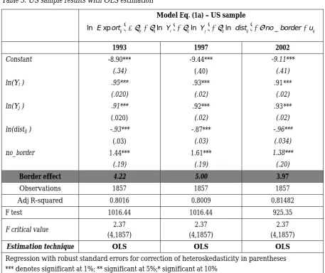
As a first robustness check, we run the equation for each of the years under consideration in our analysis separately considered [equation models (1a) and (1b)] and then by pooling all the years together in both US and EU countries’ samples [equation model (1c)] separately considered.43 _{The aim of our empirical analysis is to obtain an ‘aggregate measure’ for the} home-bias, for each of the markets under consideration. That way the information contained in each data sample can be fully exploited and summarized in a unique index. Furthermore, these two indices can be juxtaposed and serve the purpose of our comparison. The overall index for the US market is obtained through the estimation of equation (1c) and results for it are presented in Table 2 of the appendix. The same is done for the EU sample and results for it are shown in Table 3 of the appendix.

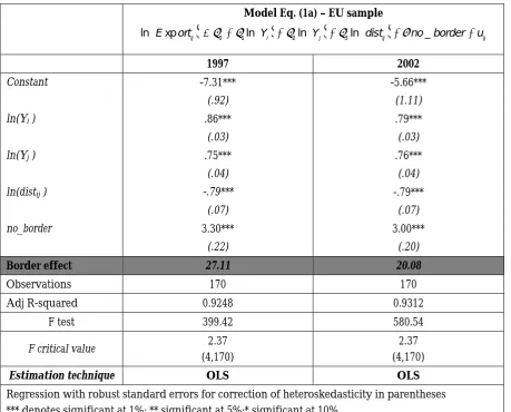
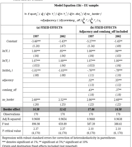
Both the OLS and panel data Fixed Effects (FE) analysis presented in Tables 2 and 3 of the appendix, precisely for model equations (1c), confirms that bilateral trade for the 50 US states and the 14 EU member states considered in our analysis is positively related to domestic income, partner income and the existence of a border in common. The distance has instead a strongly negative effect on trade flows. However, the main difference between the two techniques of estimation here employed is represented by the fact that, by direct comparison

between Table 2 and Table 3 column (2), it is possible to notice that the fixed-effect estimation technique significantly increases the overall explanatory power of the regression. In particular, it is important to remark that as a consequence of the fixed-effect estimation technique, the border effect significantly decreases in both country samples, separately considered. This conversely proves that controlling for relative prices, as suggested by Anderson and van Wincoop (2003) reduces the (omitted variable) bias in the estimates we would otherwise achieve and our equation is now more correctly specified.

For each of the years separately considered, we indeed find a home-bias which is one third less than Wolfs’ (2000) findings in the case of the US. As for the EU sample, the home-bias found is in line with Nitsch (2000) who also applies the FE techniques, but considerably lower than the home-bias found by McCallum (1995) and Helliwell (1996, 1997) and it is considerably larger than Weis’ (1996) one.44 _{Hence, the null hypothesis of the existence of no} internal barriers to trade in both US and EU internal markets is rejected. This happens despite the fact that the US Constitution expressly prohibits barriers to intra-state commerce and that, as pointed out by Nitsch (2000) for the EU sample:

if there were nothing to the notion of home country bias (and average intra-national distances, as well as internal trade volumes were approximated correctly) these basic variables would soak up all the explanatory power. There would be nothing left to attribute to a dummy variable representing intra-national trade.

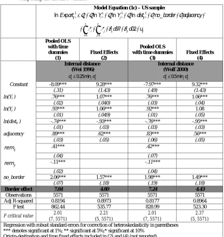
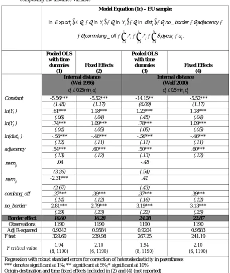
Turning to details, both scale variables, that are the GDP of both the partner countries, enter the equation highly significant and with nearly unitary coefficients.45 _{On the other hand,} distance sharply deters trade, with a coefficient close to or greater than 0.90 for the US sample,46 _{and close to 0.80 for the EU sample. A possible interpretation for this finding on the} smaller magnitude of the distance variable for the EU sample can be related to the actual distances that exist among states in the US and among states in the EU internal market. In particular, since in the former case distances in absolute values are much higher than in European countries, it might be that distances can have an even higher deterrent impact on trade in the geographically larger US market. Another robustness check employed in the equations consists of different measures of internal distance, indeed confirming previous literature findings that different ways of measuring internal distances differently affect the home-bias coefficient. In our case, for instance, the border effect coefficient would move from exp (1.57) = 4.80 to exp (1.49) = 4.43 in the US sample (see Table 2 in the annex).47 Furthermore, another robustness check, introduced in the EU sample so as to capture cultural differences that exist among European Union countries, consists of the inclusion of the ‘common language’ dummy variable. Its coefficient, significant at the 1% level, indicates that sharing a common language positively affects trade, increasing its volume (Table 3 of the annex).

The main result that emerges from our econometric analysis as shown in Tables 2 and 3 is that an average EU country still exports to itself about four times (i.e. [exp(2.79)]=16.28) as

44 _{In particular, the last statement is true despite the fact that the dataset derived in the present study}

draws upon the same databases used by Wei (1996) for what concerns the EU sample.

45_{According to Feenstra, Markusen and Rose (2001) we expect GDP’scoefficients higher than 1 for}

differentiated products, close to 1 for reference priced and around 0.80 for homogeneous products.

46 _{Which is bracketed by the elasticities found by Wolf (-1.00), by the OECD (-0.870) and the}

Canada-US (-1.38) datasets

47 _{Another robustness check realized during estimation was to include remoteness variables as defined}

much as a random US state does (i.e. [exp(1.57)]=4.80). Note that this home-bias result remains, although the equation model controls for sizes, distance, common language, common border and time and country-specific fixed-effects.48 _{This finding shows that} despite the numerous attempts to improve economic integration within the EU internal market, its potential has not been fully exploited yet. This is particularly clear when the overall index found for the US market is taken as a benchmark.

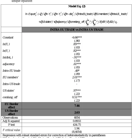
Once the overall index for each of the markets has been found as separate fixed-effect estimation of equation (1c), we consider another exercise. As explained before, a unique balanced sample can be obtained by pooling together the US and the EU data so that better estimates for the variable coefficients can be obtained by applying the same FE estimation technique so far considered. Results are presented in Table 4 of the appendix.

The test of home-bias through the equation model (2) indeed delivers us some additional information. The coefficient of the Intra-EU trade, as positively signed and significant at the 10% level tells us that the volumes of trade between two EU countries were actually higher than a random pair of US states, ceteris paribus. This can be interpreted as a sign of the fact that the various attempts to deliver a unique and functioning market for the EU member states have been to some extent successful, fostering trade patterns.

In general, however, the findings reported in Table 4 in the annex deliver results for incomes, distances and common language coefficients that are in line with those found in the previous sections. Nevertheless, when we turn to the border effect coefficient, we can see that this is now (proportionally) smaller than it was before when the two markets were studied separately,49 _{and this particularly holds for the EU market. In particular, our evidence shows} that while a random state in the US tends to exchange

[

exp(0.97)

]

=2.63 times more towards

itself than towards other states, the same figure for an EU member state is

[

exp(2.01)

]

=7.46,

thus almost three times greater against the four times as previously found. Therefore, similar to what has been obtained before, EU internal market home-bias is much higher than the US market home-bias, even if of a magnitude smaller (from three to four times as much) than the result in previous sections.

3.2

Possible interpretations of the results

This section aims at delivering some possible economic interpretations of the reason why the EU border effect results are so much higher than the US border effect results.

The ‘home-bias’ literature represents a new and possibly interesting alternative way of studying the intensity of market integration, compared to the traditional indicators such as intra-group trade flows in goods and services (as a ratio of other variables) or the stocks and flows of FDI or other forms of cross-border intra-group mobility, or, for that matter, price convergence. This CEPS Working Document attempts to contribute to the study of EU home-bias by direct comparison with the US in two variants. The finding is that EU countries have a home-bias some three to four times that of US states.

This home-bias is constructed in such a way that it can be regarded as a measure of the (lack of) depth of market integration. However, the difficulty of this literature remains that there is no underlying economic theory that is tested or verified. It is little more than a sophisticated empirical observation, after controlling for determinants such as language and contiguity

48 _{And Wei (1996) internal distances are considered for both country samples.}

49 _{This might also be due to the fact that the observations in equation 3 refer only to two years (1997}

between EU countries. All sorts of explanations (can) compete in order to underpin these results. Thus, prior education and habits might cause domestic traders and businesses to perform transactions more frequently with their national partners than some benchmark might lead one to expect. Thus, networks might maintain a form of trust and comfort in doing business that is possibly efficient since it will rarely require a lot of formal contracting and verification.50 _{Thus, there might be remaining barriers in the EU that have not or not} fully been removed (e.g. public procurement is formally under detailed EU rules, but there is doubt whether they work well or as intended; and public purchases and works do represent some 16% of EU GDP). There might therefore be implementation problems in EU law (as is well-known). There might be more or less serious anti-competitive practices, not caught by anti-trust authorities, whether EU or national, including market dividing practices. It is also suspected that market integration in the EU - though ‘deep’ by any comparison with any other instance of economic regionalism in the world (not the USA, because that is of course a single country) – is anything but complete, as the repeated attempts to further deepen and widen the EU internal market show.51 _{Finally, there is a lingering suspicion, with more than} anecdotal evidence, that the internal market cannot always work itself out on trade and investment (and mobility of workers) as expected due to rigidities in national markets which fall outside the scope of the conferred powers at EU level. For all these reasons and more, the understanding of home-bias is an open question.

Therefore, it is less than clear that the considerable home-bias the EU internal market is still suffering from is largely due to formal regulatory or illegal (anti-competitive or regulatory) barriers. Moreover, some barriers do exist which, under current arrangements, are legal in the EU (although in an economy serving as the benchmark for home-bias, they should no longer exist). Still, the extent of the home-bias in the EU, after almost 60 years of economic integration, is so great that a further deepening and widening (of the scope) of the internal market would undoubtedly help to induce a major reduction. The extent of such a reduction cannot be read from the present econometric exercise, unfortunately.

Another explanation for the higher EU border trade was found, in the present analysis, in the significance of the ‘common language’ variable. All the findings about it confirm that a different language spoken by two partner countries has a highly negative effect on trade. This is one of the peculiarities of the EU when compared to the US for example, and it is still difficult to imagine how an even better diffusion of (a) common EU language(s) would firstly be accepted by the member states and secondly enable us to overcome any of the difficulties that those differences among member states can create in terms of trade facilitation. Moreover, together with the language, networks, habits, cultural affinity and ‘ways of doing business’ might all be relevant barriers as well and are reflected for instance in different bureaucratic procedures (e.g. the so-called red tape), that will take even longer to disappear, if it ever does. This is another aspect that further investigations should try to explore.52

Thirdly, only aggregated data (i.e. not at the industry level) is considered in the current analysis. Nevertheless, authors that have been able to work at the industry level on this

50 _{See Combes, Lafourcade & Mayer, 2005 for strong evidence on certain specific French networks of}

migrants.

51 See e.g. Pelkmans, 2010 on the weak 2007 Internal Market Review, which followed two consecutive internal market strategies under Commissioner Bolkestein ; and Pelkmans, 2011 for the “Case for more single market” in response to COM (2010) 608 of 27 October 2010, Towards a Single Market Act.

52 _{See Alesina and Gavazzi (2006) in whose book the cost of doing business in the two-country}

topic53 _{have systematically found that certain industries, such as oil refining or construction} materials, were characterized by a very high border effect due to the higher transportation costs related to them. Consequently, our different results for the EU and the US could also be a reflection of a different composition of their industry networks that could be explored in further studies.

Last but not least, separate consideration and the estimation of markets for goods and markets for services would be particularly meaningful in future analyses.

4.

Conclusions

This CEPS Working Document has performed an empirical test of home-bias effect at the intra-state level in the US and EU internal markets, which are by conventional wisdom the two most fully integrated regions of the world. Using the standard gravity equation model, the analysis has been approached from two different points.

First, estimations based on single equation cross-sectional analysis for each of the markets separately considered support the hypothesis of home-bias effect. This means that trade flows at the intra-national level are ‘excessively’ high when compared to the level of commerce towards other countries, once direct distance and economic size are accounted for. Nevertheless, the finding of a home-bias coefficient obtained through the simplest, standard form of gravity equation delivers estimates that are biased due to omitted variable problems. The hypothesis of no home-bias effect has been further tested through a panel with country-specific fixed effect estimation, which represents the second approach. In this case the data also supports the hypothesis of home-bias effect. The new estimates obtained are more likely to reflect the real level of friction to trade at the intra-state level, further controlling for common language and a common land border.

Finally, inclusion of time dummies, besides the already implemented origin-destination fixed effect estimation, and the inclusion of both EU and US data samples in a unique equation allowed us to find overall indicators for the border barrier in both the US and EU markets, thus making them more (directly) comparable. These aspects are novel features of the present study.

53 _{Chen, Natalie (2004), “Intra-national versus international trade in the European Union: why do}

References

Alesina, Alberto and Francesco Giavazzi (2006), The Future of Europe: Reform or Decline, Cambridge, MA: MIT Press.

Aitken, N.D. (1973), “The Effect of the EEC and EFTA on European Trade: ATemporal Cross-Section Analysis”, American Economic Review, Vol. 63, No. 5, pp. 881-892.

Anderson, James (1979), “A Theoretical Foundation for the Gravity Equation”, American Economic Review, Vol. 69, pp. 106-116.

Anderson, James and Eric van Wincoop (2003), “Gravity with Gravitas: A solution to the Border Puzzle”, The American Economic Review, Vol. 93, No. 1, pp. 170-192.

Anderson, James and Eric van Wincoop (2004), “Trade Costs”, Journal of Economic Literature, Vol. 42, No. 3, September, pp. 691-751.

Baldwin, Richard and Charles Wyplosz (2006), The Economics of European Integration, 2nd _Ed., Maidenhead, Berkshire: McGraw-Hill.

Balta, Narcissa and Juan Delgado (2009), “Home Bias and Market Integration in the EU”, CESifo Economic Studies, Vol. 55, No. 1/2009, pp. 110-144.

Bergstrand, Jeffrey (1985), “The Gravity equation in International Trade: Some Microeconomic Foundations and Empirical Evidence”, The Review of Economics and Statistics, Vol. 67, pp. 474-481.

Bayoumi, Tamim and Barry Eichengreen (1995), “Is Regionalism Simply a Diversion? Evidence from the Evolution of the EC and EFTA”, CEPR Discussion Paper No. 1294, Centre for Economic Policy Research, London.

Chen, Natalie (2004), “Intra-national versus international trade in the European Union: why do national borders matter?”, Journal of International Economics, Vol. 63, pp. 93-118. Davis, Donald (1996), “Intra-industry Trade”, Journal of International Economics, Vol. 39,

pp.3-4.

Deardorff, Alan (1994), “Testing Trade Theories and Predicting Trade Flows”, in R. Jones and P. Kenen (eds), Handbook of international Economics, vol. 1, Amsterdam: Elsevier.

Deardorff, Alan (1995), “Determinants of Bilateral Trade: Does Gravity work in a Neoclassical World?”, in Jeffrey Frankel (ed.), Regionalization of The World Economy, Chicago: University of Chicago Press.

Delgado, Juan (2008), Single Market Trials Home Bias, Bruegel Policy Brief No. 38, Bruegel, Brussels.

De Grauwe, Paul (1988), “Exchange Rate Volatility and the Slowdown in growth of international trade”, IMF Staff papers, Vol. 35, No. 1, March.

Frankel, Jeffrey, Stein Ernesto and Wei Shang-Jin (1995), “Trading Blocks and the Americas”, Journal of Development Economics, Vol. 47, No. 1, pp. 61-96.

Head, Keith and Thierry Mayer (2000), “Non-Europe: The Magnitude and Causes of Market fragmentation in the EU”, Review of World Economics, Vol. 136, No. 2, pp. 284-314.

Head, Keith (2003), “Gravity for Beginners”, Mimeo, Vancouver: University of British Columbia.

Hillberry, Russell and David Hummels (2003), “Intranational Home Bias: some explanations”, The Review of Economics and Statistics, Vol. 85, No. 4, pp. 1089-1092.

Helliwell, John F. (1995), “National Borders still matter for Trade” (with John McCallum), Policy Options/Options Politiques, Vol. 16, No. 5, Special issue July-August, pp. 44-48. Helliwell, John F. (1996), “Do national borders matter for Quebec’s trade?”, Canadian Journal

of Economics, Vol. 29, No. 3, pp. 507-22.

Helliwell, John F. (1997), How Much Do National Borders Matter?, Washington, D.C.: Brookings Institution.

Helpman, Elhanan and Paul Krugman (1985), Market Structure and Foreign Trade, Cambridge, MA: MIT Press.

Hummels, David (1999), “Toward a Geography of Trade Costs”, Mimeo, Purdue University. McCallum, John (1995), “National Borders matter: Canada-US regional trade patterns”,

American Economic Review, Vol. 85, pp. 615-23.

Linnenman, Hans (1969), “Trade Flows and Geographical Distance, or the Importance of being Neighbour”, in H.C. Bos (ed.), Towards Balanced International Growth, Amsterdam: North Holland, pp. 111-128.

Nitsch, Volker (2000), “National Borders and International Trade: Evidence from the European Union”, Canadian Journal of Economics, Vol. 33, pp. 1091-1105.

Pelkmans, Jacques (2008), Economic approaches of the Internal Market, Bruges European Economic Research papers, BEER paper n°13 2008.

Pelkmans, Jacques (2011) The case for ‘more single market’, CEPS Policy Brief No. 234, Centre for European Policy Studies, Brussels.

Wei, Shang-Jin (1996), Intra-national versus international trade: how stubborn are nations in global integration?, NBER Working Paper No. 5531, National Bureau of Economic Research, Cambridge, MA.

Wolf, Holger C. (1997), Patterns of intra-and inter-state trade, NBER Working paper No. 5939, National Bureau of Economic Research, Cambridge, MA.

Wolf, Holger C. (2000), “Intranational Home Bias in Trade”, The Review of Economics and Statistics, Vol. 82, No. 4, pp. 555-563.

World Bank Indicators, (2007), http://data.worldbank.org/indicator.

[image:24.595.57.784.89.507.2]

Annex

Table 1. A summary description of the variables employed in the analysis

Variable Description Source

US EU

Expij Exports from state i to state j, US mln dollars _{(current $ values)} Exports from state i to state j, US mln of dollars _{(current $values)} RITA IMF (DOTS 2007)

Expii/Expjj Imports from each country to itself, mln of US _{dollars (current $ values)} Following Wei (1996), a three steps procedure is applied (own calculation):

(1) The good part of GDP (or GGDP) is computed as: GGDP=GDP-service-transport (2) Calculation of shipment-to-value added ratios (3) Total goods production = (Shipment/value added ratio) * GGDP

RITA World Bank Indicators (2007) http://data.worldbank.org/in

dicator

OECD Structural Statistics for _{Industry and Services (2007)}

Yi Gross state product (state i), US mln dollars (current $ values) US census gov abstract

World Bank Indicators (2007)

Yj Gross state product (state j), US mln dollars (current $ values)

distij

Distance calculated as a great circle distance (own

calculation) following the Haversine formula

R.V. Sinnot, "Virtues of the Haversine" Sky and telescope, vol. 68/2(1984) p.159.

http://team.univ-paris1.fr/

teamperso/mayer/thierry.htm. World-gaezetteer website _{for geographical} coordinates and www.indo.com/distance

http://econ.sciences-po.fr/staff/thierry-mayer

(dist ii-jj) Internal distances are calculated following Wei (1996): dii=0.25minjdij and Wolf (2000): dii=0.5minjdij

no_border Dummy which is equal to 1 for intrastate shipments.

i

α Dummy equal to1 if i=1 (where i =1,...,I,and 50

I= )

Dummy equal to1 if i=1 (where i =1,...,I,and 14

I = )

j

α Dummy equal to1 if j=1 (where j =1,...,N,and 51

J = )

Dummy equal to1 if j=1 (where j =1,...,J,and 12 (13)

J= )

Adjacency Dummy variable which indicates whether the two country have a border in common www.netstate.com/states http://econ.sciences-_{po.fr/staff/thierry-mayer}

remij-remji

Remoteness variable from state I to state j measured as the GDP weighted average distance between state i and all the state except j [Helliwell 1998]

www.indo.com/distance www.indo.com/distance

comlang_off Dummy=1 for a common OFFICIAL language

http://econ.sciences-po.fr/staff/thierry-mayer

i

dyear Time dummy indicator(s)

1 3

1,

e ij

ij ji

k k j k

D i s t

r m r e m

Y

= < >

=

∑

=

49

1,

e ij ij e ji

k k j k

Dist

r m r m

Y = <>