Evaluation of subdivision methods used in octree ray tracing algorithms

RIT Scholar Works

Theses

Thesis/Dissertation Collections

1998

Evaluation of subdivision methods used in octree

ray tracing algorithms

Scott Brown

Follow this and additional works at:

http://scholarworks.rit.edu/theses

This Thesis is brought to you for free and open access by the Thesis/Dissertation Collections at RIT Scholar Works. It has been accepted for inclusion

in Theses by an authorized administrator of RIT Scholar Works. For more information, please contact

[email protected].

Recommended Citation

Computer Science Department

Evaluation of Subdivision Methods

used in Octree Ray Tracing Algorithms

by

Scott D. Brown

A thesis, submitted to

The Faculty of the Computer Science Department

in partial fulfillment of the requirements for the degree of

Master of Science in Computer Science

Approved by:

Professor Nan Schaller

Professor John Schott

Professor Stanislaw Radziszowski

used

in

Octree

Ray Tracing

Algorithms

Scott

D. Brown

ABSTRACT

Key

words:

ray

tracing

optimization,

non-uniform spatial

subdivision, octree, octtree,

octree subdivision methods.

The

non-uniformspatial subdivision

technique

refined

by

Andrew Glassner

[Glassner

1984]

minimizes

facet

intersection

tests

(i)

by

automatically generating

a

density

dependent

spatial

hierarchy

of

facet

regions

(called

an

octree)

and

(ii)

by

only

testing

facets

in

regions

along

the

path of

the

ray.

Past

research

has

addressed optimization of

the

octree

ray

tracing

process

by

separately

improving

both

the

octree

traversal

method and

facet

intersection

algorithms.

This

author attempted

to

further

improve

the

overall approach

by

attempting to

identify

new octree construction methods

that

would

decrease

the

number of

traversals

required

to

render

the

scene.

This

research

focused

on

the

subdivision

technique

used

in constructing

the

octree.

The

conventional

Glassner

algorithm utilizes cubic octants

that

can result

in

a

large

population of

empty

octants when

rendering

scenes

containing

localized

regions with

high

facet

density.

Sparse

octrees

(containing

significant numbers of

empty

octants)

were

believed

to

hinder

performance of

the

facet

traversal

algorithm.

As

an alternative

to the

conventional cubic

algorithm,

the

performance

benefits

of non-cubic octants were

investigated.

Octrees

constructed with "rectangular" octants which more

closely

bound

the

scene were

tested

as one alternative

to

the

cubic octants method.

As

a second

alternative, this

author proposed and

implemented

an "ideal-cut" subdivision algorithm

that

subdivides

the

parentoctant

through

the

mean

location

of

the

facets

contained

in the

octant.

For

the

scenes

tested,

the

"conventional" cubic algorithm was shown

to

perform

better

than

either alternative

method,

although, it

was also shown

to

suffer

from

memory

and run-time explosions on some scenes.

The

"rectangular"

octant algorithm

consistently

approached

the

run-times produced

by

the

"cubic"

method.

Since,

the

"rectangular" method

defaults

to

the

"cubic" method

for

scenes with

1:1:1

aspect

ratios, the

"rectangular"

method must

be

considered as a reasonable alternative

in rendering

applications.

The

"ideal-cut"

subdivision algorithm was shown

to

minimize

the

empty

octants and overall octree

depth,

however,

an

increased

numberof

facet

intersection

tests

were required.

In

an attempt

to

identify

the

algorithm or scene

characteristics

that

gave rise

to the

variation

in

algorithm

performance,

anextensivecorrelation analysis was performed.

However,

an a-priori scene characteristic

to

automatically

select

the

most efficient algorithm

used in Octree Ray Tracing Algorithms

I, Scott D. Brown, hereby grant permission to the Wallace Library of the Rochester

Institute of Technology to reproduce my thesis in whole or in part. Any reproduction will

not be for commercial use or profit.

I

wish

to thank

Nan

Schaller for

being

my

advisor

during

the

course of

this

Thesis

and

the Independent

Study

that

started

this

whole

project,

but

mostly

for her

patience

to

comment on

the

many

revisions of

this

document.

I

also wish

to thank

Stanislaw Radziszowski for

bringing

his

knowledge

of computational

complexity

to

a computer graphics related

thesis.

My

thanks

also go

to

Pat Fleckenstein for

helping

me

debug

my

original code.

Finally,

my

sincerest

thanks to

John

Schott for

supporting my

efforts

to

complete

this

degree

and

for his

Contents

1

Introduction

and

Background

1

1.1

Ray Tracing

Optimizations

1

1.2

Octree Creation

and

Ray Tracing

3

1.3

Preliminary

Observations

7

1.4

Statement

of

Hypothesis

9

1.5

Summary

of

Octant Subdivision Methods

9

1.5.1

The Conventional Algorithm

10

1.5.2

The Rectangular

Octant Algorithm

10

1.5.3

The

Ideal

Octant Algorithm

11

1.6

Statement

of

Work

12

1.6.1

Implementation

12

1.6.2

Data Creation

12

1.6.3

Data Analysis

12

2

Implementation

13

2.1

Conventional Subdivision Algorithm

13

2.2

Ideal

Cut Subdivision Algorithm

14

3

Results

and

Analysis

1'

3.1

Test Results

17

3.1.1

Statistical Scene #1

18

3.1.2

Statistical Scene #2

21

3.1.3

Statistical Scene #3

23

3.1.4

Geometric Scene

26

3.1.5

Bomber Scene

28

3.1.6

Forest

Scene

30

3.1.7

Terrain

Scene

32

3.1.8

Fighter

Scene

34

3.1.9

Urban

Scene

36

3.2

General Analysis

38

3.2.1

Run-Time Performance

38

3.2.2

Octree Build Time

and

Memory

Usage

38

3.3

Correlation Analysis

40

3.3.1

Octree Size

versus

Run-Time

43

3.3.2

Octree Size

versus

Octant Traversal

45

3.3.3

Octree Size

versus

Facet Intersection Tests

49

3.3.4

Empty

Octant Population

versus

Run-Time

51

3.4

Predicting

the

Best

Algorithm

54

3.4.1

Using

scene size

54

4

Conclusions

and

Recommendations

57

4.1

Algorithm

Summary

57

4.2

Automatic Algorithm Selection

58

4.3

Future Work

58

A

libRT Design Document

59

A.l

Abstract

59

A.2

Introduction

60

A.2.1

Project Justification

60

A.2.2

Ray Tracing

Basics

61

A. 3

Implementation Description

64

A.3.1

Supporting

Data Types

64

A.3.2

Object Storage

66

A.

3.3

Octree Creation

66

A.3.4

Ray Tracing

69

A.3. 5

Round-off

and

Precision

Strategy

73

B

Source Code

75

B.l

CreateJDctree

75

B.2

RT_0ptimize_0ctant

79

B.3

RT_Sort_Facet

83

B.4

RT_Find_0ctant

86

B.5

RT.Add_Facet_To_Octant

87

B.6

RT_Create_Sub_Octants

89

95

C

make_scene

Design

Document

95

C.l

Introduction

95

C.2

Program Definition

Qfi

C.2.1

Include Files

C.2.2

Constant

Definitions

C.2.3

Type

Definitions

97

C.2.4

Internal Function Prototypes

98

C.3

Main

Routine

"

C.3.1

Declarations

"

C.3.2

Reading

the

Input

File

"

C.3.3

Generating

the

Scene

10

C.3.4

Outputting

the

scene

to

a

file

100

C.4

Constructing

a

Facet

Distribution

101

C.4.1

Computing

the

Facet Vertices

102

C.4.2

Rotating

the

Facet

102

C.4.3

Translating

the

Facet

103

C.4.4

Computing

the

Facet Normal

103

C.4.5

Adding

the

Facet

Attributes

103

C.5

Support

Routines

103

C.5.1

Random Number Generation Routine

104

C.5. 2

Facet Rotation Routine

105

C.5.3

Facet Translation Routine

107

C.5.4

Facet Normal

Computation Routine

108

C.6

Input File

112

C.6.1

Example Input File

112

C.6.2

TAG Definitions

113

C.6.3

Input File

Reading

Routine

114

D

User's Guide

121

D.l

Introduction

121

D.2

Basic Data Types

121

D.3

Object Storage

122

D.4

Octree Creation

122

D.5

Ray Tracing

123

D.6

Prototypes for

User

Accessible Functions

124

D.7

Basic

Code Example

126

List

Figures

1.1

A 2-dimensional

example of a user

defined

bounding

box

hierarchy

and a

ray

being

traced

through the

scene

2

1.2

A

2-dimensional

example of spatialsubdivision

based

on

facet

density

and a

ray

being

traced

through the

scene

3

1.3

Creating

an octree

for

efficient

ray

tracing

4

1.4

Utilizing

an octree

to

perform

ray

tracing

6

1.5

Case A

requires

two

octants

to

be

traversed

and

five facets

to

be

checked as opposed

to

one

octant and

three

facets

in

Case B

8

1.6

Additional facet

intersection

tests

are performed

in

Case

B

that

are avoided

in

Case A

. . . .

9

1.7

A 2-dimensional

example of

the

conventional spatial subdivision

utilizing

cubic octants. ...

10

1.8

A 2-dimensional

example of

the

spatial subdivision

utilizing

non-cubic octants

11

1.9

A

2-dimensional

example of

the

spatial subdivision

utilizing

"ideal-cut" octants

11

3.1

Image

of

the

"Stat

#1"

scene

18

3.2

Image

of

the

"Stat

#2"

scene

21

3.3

Image

of

the

"Stat

#3"

scene

23

3.4

Image

of

the

"Geometric" scene

26

3.5

Image

of

the

"Bomber" scene

28

3.6

Image

of

the

"Forest" scene

30

3.7

Image

of

the

"Terrain" scene

32

3.8

Image

of

the

"Fighter"

scene

34

3.9

Image

of

the

"Urban" scene

36

A.l

Sources

of

invocation

for

the ray

tracer

library

60

A.2

A

2D

example of a user

define

bounding

box

hierarchy

and a

ray

being

traced through the

scene.

62

A. 3

A

2D

example of spatial subdivision

based

on

facet

density

and a

ray

being

traced through

the

scene

63

A.4

The

core

data

structures used

in libRT.

65

A.

5

Creating

an octree

using

a

Spatial

Sorting

Algorithm

67

A. 6

A

2D

representation of

the

four

tests

scenarios used

in the

facet-box

intersection

algorithm. .

69

A.

7

Ray

tracing

with

the

use of anoctree

70

A.8

The

ray

tracing

interface

to

libRT

71

A. 9

A

2D

representation of a

"false

termination"

List

Tables

3.1

Summary

of profiler output

for

the

"Stat

#1"

scene

19

3.2

Summary

of profiler output

for

the

"Stat

#2"

scene

22

3.3

Summary

of profiler output

for

the

"Stat

#3"

scene

24

3.4

Summary

of profiler output

for

the

"Geometric" scene

27

3.5

Summary

of profiler output

for

the

"Bomber" scene

29

3.6

Summary

of profiler output

for

the

"Forest" scene

31

3.7

Summary

of profiler output

for

the

"Terrain" scene

33

3.8

Summary

of profiler output

for

the

"Fighter"

scene

35

3.9

Summary

of profiler output

for

the

"Urban" scene

37

3.10

Average

time

and rankings

taken

to

render

the

test

scenes

38

3.11

Average

time

and rankings

taken to

construct

the

octree

39

3.12

Average

rankings

based

on size of

the

octree

40

3.13

An

example correlation computation

41

3.14

Analysis

of correlation

between

total

octree size and run-time performance

44

3.15

Analysis

of correlation

between

the total

octree size and

the

number of octant

traversals

performed

46

3.16

Analysis

of correlation

between

the

number of octant

traversals

and

the

total

run-time ....

48

3.17

Analysis

of correlation

between

total

octree size and

the

number of

facet

intersection tests

performed

50

3.18 Analysis

ofcorrelation

between

octant

traversals

and

empty

octant population

52

3.19 Analysis

of correlation

between

empty

octant population and run-time performance

53

3.20

Correlation

between

scenesize and

the

fastest

algorithm

54

Introduction

and

Background

1.1

Ray Tracing

Optimizations

Ray

tracing

is

a popular

rendering

method

because

it

simulates

the

physics of

image formation:

rays cast

from

the

simulated camera

find

the

sources of photons

that

wouldenter a real camera.

Using

simple vector

mathematics,

sources of reflections and shadows can also

be

identified

and

incorporated.

In

a minimal

algorithm,

facet

intersection

tests

must

be

performed on

every

object

in

the

scene

to

correctly

identify

the

closest surface

along

the the

ray.

For large

scenes,

this

linear

search

becomes

computationally

significant.

As

a

result,

muchof

the

research

in

the

ray

tracing

community is

focused

on strategies

to

minimize

the

number of

intersection

tests

required per

ray

trace.

A

multi-level

bounding

box

algorithm

is commonly

utilized

to

minimize

the

number of

facet intersection

tests

(see Figure

1.1)

[Clark

1976,

Rubin

and

Whitted

1980,

Weghorst

et al.

1984].

The

ray

being

traced

is

tested

for

intersection

withall of

the

bounding

volumes at

the

top

of

the

hierarchy.

If

the

ray intersects

a

volume,

then

further

intersection

tests

must

be

performed on

the

sub-volumes or

facets

contained

by

the

volume.

If

the ray

does

not

intersect

the volume, then

it

can

be

assumed

that

intersection

with

any

facets

within

the

volume

is

impossible,

and

those tests

can

be

avoided.

The

burden

of

constructing

the

bounding

box

hierarchy

is usually

placed on

the

user, requiring

additional

planning

and effort

to

create scenes.

Although

this

strategy

does

minimize

intersection

tests

whencompared

to the

global search

approach, it

has

several

limitations:

The

user

may

define

"poor"

Figure

1.1:

A

2-dimensional

example ofa user

defined

bounding

box

hierarchy

anda

ray

being

traced through

the

scene.

The

order

that

bounding

box intersection

tests

are performed

is

not optimal.

Because

there

is

not a

spatial

ranking

based

on

distance from

the

ray origin,

all

boxes

must

be

checkedat a given

level in

the

hierarchy.

To

avoid

these

limitations,

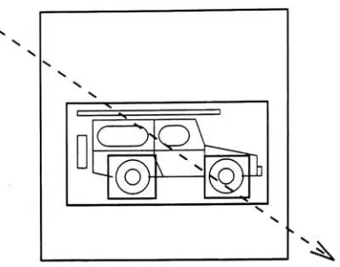
a non-uniform spatial subdivision

[Glassner

1984]

algorithm can

be

used.

This

algorithm

systematically

subdivides

the

scene

into

axis aligned

boxes

or octants

based

on

facet

density

-regions

containing

more

facets

are subdivided

into

smalleroctants

to

minimize

the

number of

intersection

tests

required per octant

(see

Figure

1.2).

The

resulting

data

structure

is

a spatial

hierarchy

of

bounding

boxes,

called an octree.

The

depth

of

the

octree

is

limited

only

by

the

amount of physical memory.

However,

as

it

will

be described

later,

the

depth

of

the

octree

does

effect

the

computational

efficiency

of

the

algorithm.

In general,

the

octree algorithm

is

more efficient

than the

user

defined

hierarchy

algorithm as

it

addresses

many

limitations

of

the

later:

The

construction of

the

octree

is automated,

and requires minimaloverhead at run-time rather

than

during

the

scene construction process.

The

number of

facets

contained

in

each octant

is

bounded

by

a user

defined

threshold

and octants

neveroverlap.

Octants

are

progressively

examined

based

on

distance from

the

origin of

the

ray.

Once

an

intersection

[image:17.551.181.373.79.230.2]

1=

I

*<-*S

/

~

"^

\

)

\

T^

-s \ x

^r

W

J

N.

4

Figure

1.2:

A 2-dimensional

example of spatial subdivision

based

on

facet

density

and a

ray

being

traced

through the

scene.

1.2

Octree Creation

and

Ray Tracing

The

spatial subdivision of

the

scene

into

an octree

is

the

required

preprocessing

stage

that

makes

the

run

time

tracing

of

the

scene more efficient

than

many

conventional

ray

tracing

techniques.

Upon

completion of

the

scene subdivision

phase,

each

leaf

node or

leaf

octant

in the

octree will contain a

list

of all

facets

that

intersect the

space

defined

by

that

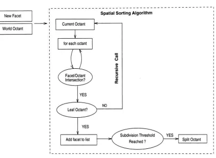
octant.

The

algorithm

for

building

the

octree

is

outlined

below

and

is

illustrated in

Figure

1.3:

The base

of

the

octree,

or

the

world

octant,

is

constructed

to

bound

all of

the

objects

in

the

scene.

The

octree

is

created

by

adding

each

facet

in

the

scene

to the

octree.

Starting

with

the

world

octant,

each

facet is

tested

against each sub-octant

for

intersection.

Each intersected

sub-octant

then

repeats

this

intersection

test

for its

sub-octants

in

a recursive

fashion. The

recursion

terminates

when a

leaf

octant

is

found,

at which point a reference

to the

facet

is

added

to

that

octant's

facet list.

All

sub-octants of an octant

intersected

by

the

facet

must

be

examined since

the

facet

may

extend over several

branches

of

the

octree.

If

the

addition of a

facet

to

a

leaf

octant exceeds

the

user

defined

subdivision

threshold then that

octant

is

split.

To

split an

octant,

eight new sub-octants are allocated and

the

facets

contained

by

the

original octant are sorted

into

eachof

the

newsub-octants.

The splitting

of

leaf

octantscontinues

untilall octants are

below

the

subdivision

threshold.

[image:18.551.180.372.78.226.2]

New

Facet

World

Octant

Spatial

Sorting

Algorithm

Current Octant

for

eachoctant

YES

YES

Add facet

to list

O

0) >

3 O a rx

NO

Subdivision

Threshold

\

YES

[image:19.551.73.495.180.490.2]

Reached

?

Split Octant

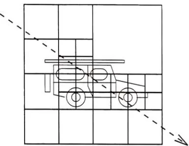
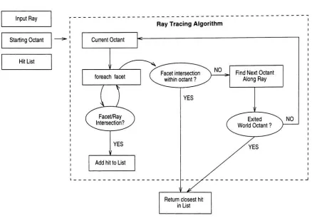
Once

the

octree

has been

constructed

for

a particular

scene,

the

procedure

for

tracing

a

ray

proceeds as

follows

(see Figure

1.4):

Ifa

starting

leaf

octant

is

not

provided,

then the

first leaf

octant

along

the

path of

the

ray is

used as

the

starting

octant.

The

ray is

tested

for

intersection

(a

hit)

with all

the

facets

within anoctant.

To

identify

the

closest

hit

to

the

ray origin,

all

hits

are stored

in

a

list

sorted

by

distance

from

the ray

origin.

In

the

event

that

no

intersections

are

found

within

the

current

octant, the

next octant

along

the

path must

be determined.

To

find

the

next octant

along

the

ray,

a search point

is

computed

in

the

neighboring

octant

along

the

pathof

the

ray.

First,

a

ray

/box

intersection

test

is

performed

to

find

the

exit point

from

the

current octant

[Haines

1991,

Kay

1986].

The

search point

is

half

the

size of

the

smallestoctant perpendicular

to

the

exited

face

of

the

current octant.

This

point

is

guaranteed

to

be

within

the

nextoctantwithout

skipping

the

smallest octant.

The

search point

is

supplied

to

the

octree search

function

and

the

octant

containing

the

point

is

identified

as

the

next octant

along

the

ray.

The

process repeats

itself

untila

facet is

intersected

or

the ray

leaves

the

world octant.

Input

Ray

Starting

Octant

Hit

List

[image:21.551.58.496.181.487.2]

Return

closest

hit

in List

1.3

Preliminary

Observations

The

performance of

the

octree

ray

tracing

method

is

dependent

upon

two

primary

operations:

(i)

octree

traversal

(moving

from

the

current octant

to the

next

along

the

path of

the

ray)

and

(ii)

facet

intersection

tests.

Since facet

intersection

algorithms

have been

heavily

investigated [Badouel

1990,

Haines

1991],

this

research

focuses

on

improving

the

octree

traversal

aspect of

the

algorithm.

Specifically,

this

author attempted

to

identify

new octree construction methods

that

would

decrease

the

number of

traversals

required

to

render

the

scene.

The

conventional octree subdivision method splits

the

octant

into

eight

(8)

sub-octants of equal size.

If

the

facets

within an octant are

extremely

localized,

one or more of

the

sub-octants will

be

over populated and must

be

split

again,

further

increasing

the

octree

depth.

Since

the

octant

traversal

algorithm must navigate a

hierarchical

tree,

deeper

octrees result

in

longer

traversal times.

When

over populated octants are

generated,

the

remaining

sub-octants are

usually sparsely

populated or

possibly

empty.

This

results

in

an

increased

probability

of

the

search

finding

an

empty

octant

(containing

no

facets

to

intersect

the

ray)

and

requiring

another search

to

be

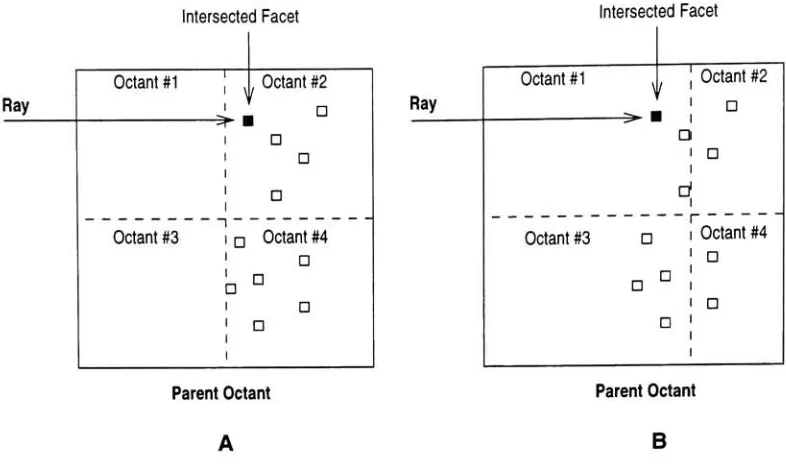
started.

Figure 1.5

illustrates

each of

these

observations.

Case A

illustrates

a scenario where

the

conventional cubic

octant method cuts

the

parent octant

through the

center.

The

ray

tracing

algorithm searchesand

identifies

octant

#1

as

the

next octant

along

the

path of

the

ray,

finds

it empty,

performs another search

to

find

octant

#2,

and

then

performs

five facet intersection

tests to

isolate

the

closest

facet. In Case

B,

the

parent octant

has been

cut

in

a

slightly

different

manner.

In

this

case, only

one octant search

is

requiredand

only

three

facets

are

tested

for

intersection

before

the

hit facet

is isolated.

These

additional computations were

avoided

because

the

parent octant

in

Case B

was subdivided

through the

average

facet

location

rather

than

through the

middle of

the

octant.

If

the

sub-octants used

in

this

example were constructed

using

the

Case

B methodology,

fewer

total

facets

would

be

examined

(since

the

first

octant

in

Case

B

contains

fewer facets

Intersected

Facet

Intersected Facet

Ray

Octant #1

Octant

#2

Octant

#3

-5f-i

i

I

ID

Octant

#4

Parent Octant

A

Ray

Octant #1

Octant #3

Octant #2

D

Octant #4

D

Parent Octant

B

Figure

1.5:

Case A

requires

two

octants

to

be

traversed

and

five facets

to

be

checked as opposed

to

one

octant and

three

facets

in

Case

B.

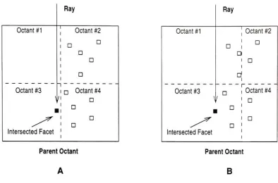
This

proposed subdivision method

does

notcome

free

of cost.

The

same

facet

population

is

illustrated

again

in

Figure

1.6,

however,

the

ray

to

be

traced

comes

from

a

different

direction.

In

this

scenario,

some

facets

are

tested

in

Case B

that

would otherwise

be

avoided

in

Case A.

However,

a change

in

performance

is only

noticed when

starting in

octants

#1

and

#3

with rays

from

these

vertical

directions.

This

does

not affect

the

efficiency

when

starting

witheither octant

#2

or

#4 from

any

direction.

Preliminary

data

showed

that

facet

intersection

tests

can

be 3

to

10

times

faster

than

octant

traversal

(depending

on

the

depth

of

the

[image:23.551.77.470.80.312.2]

Ray

Octant #1

Octant #2

!

D

D

1

?

1

?

D

Octant

#3

i

n

Octant

#4

V1

?

Intersected Facet

Octant

#1

Octant

#3

Intersected Facet

Ray

D

Q

Octant #2

D

D

Octant

#4

D

?

Parent Octant

Parent Octant

A

B

Figure

1.6:

Additional facet intersection

tests

are performed

in

Case B

that

are avoided

in

Case A

Since

the total

number of

facets

is

constant

for

a given

scene,

octrees

using

fewer

octants will

have

a

higher

number of

facets

per octant.

Although

the

average number of

facet

intersections

per octant

may increase

slightly, it is

possible

to

save enough

time

by

performing

fewer

and

faster

octant

traversals that the

resulting

overall run-time

improves.

1.4

Statement

of

Hypothesis

This

author

hypothesized

that

a subdivision method

that

attempts

to

distribute

the

facets

contained

in

an

octant

equally

to

the

child octants

may

be

more efficient.

By

doing

so, it

was

believed

that

shalloweroctrees

would

be

produced,

decreasing

the

amount of

time

spent

traversing

the

octree.

1.5

Summary

of

Octant Subdivision Methods

To

test this

hypothesis,

two

variations of

the

cubic octant style were

implemented

and

tested.

The

example

2-dimensional

facet distribution featured

in

Figure 1.7

-

1.9

is

_used

to

illustrate

the

[image:24.551.76.470.77.337.2]

traversal

efficiency

of

the

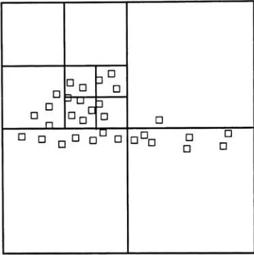
conventional algorithm and eachsubdivision variant.

1.5.1

The Conventional Algorithm

Figure 1.7 depicts the

octree generated when

using

the

conventional subdivision method

described

by

Glass

ner

in

his

original paper.

The

spatial subdivision of

the

scene

begins

by

establishing

a cube shaped octant

that

bounds

the

entire scene.

Since

this

subdivision method

bisects

filled

octants,

allsub-octants

derived

from

the

bounding

octant will also

have

a

1:1:1

aspect ratio.

For the

facet

distribution in

Figure

1.7,

a

total

of

10

octants

(two

of which are

empty)

are required

using

this

subdivision method and a subdivision

threshold

of

8

facets.

D D

D

0

n

DD

3 D 3 U ₁

D

D _D D D

DD

D

D

[image:25.551.185.364.250.430.2]

s

s

Figure 1.7:

A

2-dimensional

example of

the

conventional spatialsubdivision

utilizing

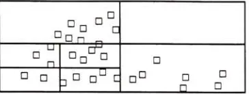
cubic octants.

1.5.2

The Rectangular

Octant

Algorithm

The

first

variant uses

non-cubic,

or rectangular octants.

In this

implementation,

the

worldoctant

is

created

to

enclose

the

maximum extents of

the

scene.

All derived

sub-octants will

feature

the

same aspect ratio as

the

bounding

octant.

Since

the

worldoctant

tightly

wraps

the

scene, the

author

hypothesized

that any

subsequent subdivisions will

have

a

higher

probability

of

separating

localized

concentrations of

facets

and would

possibly

avoid

both

overfilled and

empty

octants

(see Figure

1.8).

For

the

facet

distribution in

Figure

1.8,

a

total

of of

7

octants

(one

of which

is empty)

are required

using

IT ?

n

D^o

_a

?? a a

n n

a a ,? _DUC

Figure

1.8:

A

2-dimensional

example of

the

spatial subdivision

utilizing

non-cubic octants.

1.5.3

The

Ideal Octant

Algorithm

The

third

variation splits

the

octant

through the

mean

location

of

the

facets

contained

by

the octant,

and

is

referred

to

as

the

ideal-cut

algorithm.

This

algorithm requires

maintaining

the

mean

location

of

facets

contained

by

a given octant as

the

octant

is

filled. To balance

the

population of

facets

in

the sub-octants, the

parent octant

is

divided

through the

average

location

of all

the

facets

contained

by

the

octant.

Therefore,

every

facet

must

be

sorted

into

the

octants at a given

level before

subdivision can

take

place

(see

Figure

1.9).

The

sorting

approach used

by

the

ideal-cut

algorithm changed

the

design

of

the

facet

sorting

aspect of octree construction since

the

octant cannot

be

properly

cut until

the

meanof all

the

facets

intersecting

the

octant

is determined. In contrast,

the

previous

two

algorithms can split

the

octant once

the

octant

has

reached

the

subdivision

threshold.

The details

of

the

octreecreation

using

the

ideal-cut

algorithm

is

described

in detail

in

Chapter

2.

For

the

facet distribution

in

Figure

1.9,

a

total

of of

4

octants

(none

of which are

empty)

are required

using

this

subdivision methodand a subdivision

threshold

of

8

facets.

'e

D

D

Figure

1.9:

A

2-dimensional

example of

the

spatial subdivision

utilizing

"ideal-cut"

[image:26.551.186.368.80.149.2] [image:26.551.184.369.433.502.2]

1.6

Statement

of

Work

1.6.1

Implementation

Although

the

octree

ray

tracing

library

had

already

been

completed as part of another

effort,

additional

modificationswere made

during

the

course of

this

research.

Specifically,

these

modifications

included:

The

addition of counters

to

keep

track

of

(%)

the total

number of

octants,

(ii)

the

number of

empty

octants and

(Hi)

the

average number of

facets

per octant.

Implementation

of

the

"ideal-cut" subdivisionmethod.

This

required

keeping

track

of

the

dimensional

means of

facets

intersecting

each octant

for

use

during

octant

subdivision,

and

implementing

the

new

octree creation algorithm which utilizes a

different

sorting

approach.

Implementation

of

the

pseudo-random scene generation

tool to

create

test

scenes

(see Appendix C).

The

details

of

the

modifications required

for

this

researchare

described

in

Chapter

2.

1.6.2

Data Creation

The

modified subdivision methods were added

to the

libRT

ray

tracing

library. The

author

currently

has

this

library

installed

in the

DIRSIG

synthetic

image

generation model.

DIRSIG

is

a

high

radiometric

fidelity

multi-spectral

rendering

environment

that

can require

100

-

150

_rays

to

be

traced

for

_{each rendered pixel}

[Schott

et al.].

The

three

different

octree algorithms

(cubic

octants,

non-cubic

octants,

and

ideal-cut octants)

were each

tested

on nine

(9)

test

scenes.

Three

(3)

of

the

test

scenes were

statistically

generated

to test the

various

strengths ofeach subdivision algorithm.

The

remaining

six

(6)

scenes were

readily

available

DIRSIG

scenes.

A description

and

rendering

of each scene

is

presented with

the

scene

by

scene analysis

in

Chapter

3.

1.6.3

Data Analysis

All

of

the

collected

data

and

resulting

analysis are presented

in

Chapter

3.

Important

run-time values

for

Implementation

The

research

in

this

effort addressed

the

performance of

three

octant subdivisionmethods.

This

chapter

describes

the

implementation

differences between

the

creation of an octree

using

either

the

"cubic" or

"rect

angular"

subdivision method and

the

"ideal-cut" subdivision method.

It

should

be

pointedout

that there

are no

differences between

the

various algorithms with respect

to the

ray

tracing

process.

2.1

The Conventional Subdivision Algorithm

At

the

core of

the

conventional "cubic"

octree creation algorithm

is

a

"spatial

sorting"

algorithm

that

addsa

reference

to

any

leaf

octant

that

intersects

a given

facet.

Pseudo-code for

this

recursive

facet

sorting

routine

is

outlined

below:

RT.Sort

.Facet

(

RT.OCTANT *octant, RT_FACET

*facet

)

-C

if

(

Octant_Is_A_Leaf

(

octant

)) {

RT_Add_Facet_To_Octant(

octant,

facet

)

}

else -[

foreach(

suboctant

) {

if(

RT_Facet_Box_Intersect

(

suboctant,

facet

)) {

RT.Sort

.Facet

(

suboctant,

facet

)

>

}

The

routine

RT_Add_Facet_To_Octant

adds

the

facet

reference

to the

current

leaf

octant and checks

if the

facet

count

for

that

octant exceeds

the

subdivisionthreshold.

If

it

does,

the

octant

is

split

into

8

sub-octants

and all

the

facets

in

the

original octant are re-sorted

into

the

new sub-octants.

The

additionof

facets

to

the

octree

then

continues.

2.2

The Ideal

Cut

Subdivision Algorithm

The "ideal

cut"

subdivision method must utilize a

slightly different

approach

to

constructing

the

octree.

To

ideally

cut

the

octant,

the

mean

facet

location

all of

the

facets

intersecting

the

octant

be determined.

Therefore,

all of

the

facets

intersecting

an octant must

be

sorted

into

that

octant

before

the

octant can

be

split.

In

contrast, the

"cubic"

and "rectangular"subdivision methods can split an octant once

the

threshold

is

reached,

(a detailed

description

of

the

conventional octree creation algorithm was presented

in

Section

1.2).

An

important

modification

to

the

spatial

sorting

routine was

to maintaining

the

mean

location

of all

the

facets

contained

in

the

octant.

The

computationof

the

mean

location

does

not

include

facets

that

extend past

the

extents of

the

octant.

This is

because

this

algorithmattempts

to

split

up localized

facet

concentrations

within

the

octant.

The

algorithm

for

the

"ideal

cut"

subdivision method can

be described

by

a simple recursive process.

The

process

is

seeded

by

adding

all of

the

facets

in the

scene

to

the

world octant.

If the

numberof

facets

in

the

current octant exceeds

the

subdivision

threshold,

sub-octants are created

that

cut

through the

average

location

of

the

facets

within

the

octant.

The facet

storage area

in

the

sub-octants must

be

made

large

enough

to

hold

all of

the

facets

that

intersected

the

parent octant

(a

worst case scenario).

All

of

the

facets

are

then

sorted

into

the

child

octants,

and

the

old

facet list

is

de-allocated.

This

process

is

repeated

for

each sub-octant of

the

octant.

If

the

number of

facets

in the

current octant

does

not exceed

the

subdivision

threshold,

then the

size

The

following

section contains pseudo-code

for

the

"ideal

cut"

subdivision algorithm

previously described:

RT_0ptimize_0ctant(

RT.OCTANT

*octant

)

{

if(

Octant.Is.OverfilledC

octant

)) {

RT_Create_Sub_Octants(

octant,

octant->mean,

octant->sub_octants

)

foreach(

facet

in

octant->facet_list

) {

RT.Sort

.Facet

( facet,

octant

);

>

Free_Facet_List(

octant->facet_list

);

foreach(

sub.octant

in

octant->sub_octants

) {

RT_0ptimize_0ctant(

sub.octant

);

}

}

else

{

New_Facet_List(

octant->f

acet.count,

new.facet.list

)

foreach(

facet

in

octant->facet_list

){

Add.FacetC facet,

new.facet.list

)

}

Free_Facet_List(

octant->facet_list

);

octant->f acet.list =

new.facet.list;

}

}

Results

and

Analysis

3.1

Test Results

The

octree

ray

tracer

was run on nine

(9)

test

scenes

to

compile

the

results presented

in

this

document.

The first

three

(3)

scenes consist of simple statistical

distributions

of

facets

generated

by

the

make_scene

utility

(see Appendix C). These

scenes were

specifically

constructed

to

isolate

the

differences

in

the three

(3)

octant subdivision methods

being

studied.

These

statisticalscenes present a significant challenge

to

any

ray

tracing

algorithm

because

they

consist of

extremely

dense

and uncorrected

fields

of

facets.

The

remaining

scenes were

readily available,

"real-world" scenes

that this

author

feels

represent

the

size and

complexity

of

facetized

scenes

that

may

be

of

interest to

people

in

the

graphics

field

today.

The

following

sub-sections summarize

the

data

collected

for

each scene.

Each

scene was run with each of

the three

(3)

octant subdivisionvariants.

Each

section

includes

a

brief

description

of

the scene,

an example

image

of

the scene,

and

the

results

tabulated

from

the

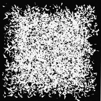
profiler output.

3.1.1

Statistical Scene

#1

Description

The

scene rendered

in

Figure

3.1

was

specifically designed

so

that

all

three

subdivision algorithms would perform similarly.

The

scene

is

a cube

uniformly

filled

with

5,000 facets

of various sizes and orientations.

Figure

3.1:

Image

of

the

"Stat

#1" scene.

This statistically

generated scene was created

using

the

following

_{parameters extracted}

directly

from

the

make_scene

input file:

DIST.ENTRY.BEGIN

TYPE

=

UNIFORM

COUNT

=

5000

AVERAGE.SIZE

=

500.0

DELTA.SIZE

=

250.0

AVERAGE.X

=0.0

DELTA.X

=

10000.0

AVERAGE.Y

=0.0

DELTA.Y

=

10000.0

AVERAGE.Z

=0.0

DELTA.Z

=

10000.0

[image:33.551.176.374.177.375.2]

Total

number of

facets

10,000

Performance

Metric

Octant Styles

Best

Performance

CUBE

RECT

IDEAL

Octree

build

time

5.51

5.51

4.83

IDEAL

Total

numberof octants

Number

of

empty

octants

2079

2

1855

0

1401

2

IDEAL

RECT

Fraction

of

empty

octants

0.001

0.000

0.002

RECT

Number

of octant searches

Octant

search

time

19,060,515

247.65

19,035,334

244.43

17,445,697

311.26

IDEAL

RECT

Number

of

facets

tested

Facet

test time

217,494,289

885.97

217,412,595

894.25

252,524,941

1043.80

RECT

CUBE

Total

run

time

1860.11

1860.14

2104.24

CUBE

Table

3.1:

Summary

of profiler output

for

the

"Stat

#1" scene.

Observations

Table

3.1

summarizes

the

performance of each algorithm

for

this

scene.

Since

the

scene consists of a square

cube

filled

with

facets,

the

worldoctant

for

all

three

algorithmsshould

be

the

same

size,

thereby

minimizing

the

differences

between

the

CUBE

and

RECT

algorithms.

However,

the

size of

the

octrees

for

these two

algorithms

is surprisingly

different. The

worldoctant size was verified

to

be

only slightly

different

because

the

extents of

the

randomly

generated

facet

population was not

exactly

a cube.

This

small

difference

was

found

to

be

responsible

for

this

rather

large difference

in

octree size.

Although

the

octree sizes were

very

different,

the total time

spenton octree

traversal

only

changed

by

approximately 1%. For

this

scene,

the CUBE

algorithm

had

the

best

run-time,

however,

the

run-time

difference between

the

CUBE

and

RECT

algorithms

is

negligible.

The

octree created

by

the

IDEAL

algorithm wasalso

bound

by

a worldoctant of similar size.

Since

the

facets

are

uniformly distributed

within

the

world

octant,

the IDEAL

should cut

the

octants

through the

middle

in

the

same manner as

the CUBE

and

RECT

algorithms.

Instead,

the IDEAL

algorithm was

found

to take

advantageof

localized

density

variations,

and most octants were not cut

through the

middle.

As

a

result,

this

method minimized

the

number of octants required

to

store

the

scene

(using

significantly

less

octants

than the

other

two

methods).

However,

the

overall performance of

this

algorithm suffers

because

the

lower

Summary

The

observations

for

this

scene can

be

summarized as:

The

CUBE

and

RECT

methods produced comparable results.

The

IDEAL

method produced

the

smallest octree

but

tested

more

facets

than the

other

two

algorithms.

A

small

difference

in the

extents of

the

world octant

for

the CUBE

and

RECT

methods resulted

in

dramatically

different

octree sizes.

This large difference

made

only

a slight change

in

the

efficiency

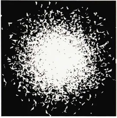
of

3.1.2

Statistical Scene #2

Description

The

scene rendered

in

Figure

3.2 is approximately

4,000

units per side and contains

5,000

facets

ofvarious

sizes and orientations.

The

density

of

facets decreases

with

distance from

the

center of

the

scene

following

a

Gaussian distribution.

Figure

3.2:

Image

of

the

"Stat

#2" scene.

This

scene was generated

using

the

following

parameters extracted

directly

from

the

make_scene

input

file:

DIST.ENTRY.BEGIN

TYPE

=

GAUSSIAN

COUNT

=

5000

AVERAGE.SIZE

=

500.0

DELTA.SIZE

=

250.0

AVERAGE.X

=0.0

DELTA.X

=

4000.0

AVERAGE.Y

=0.0

DELTA.Y

=

4000.0

AVERAGE.Z

=0.0

DELTA.Z

=

4000.0

[image:36.551.175.378.186.391.2]

Total

number of

facets

10,000

Performance

Metric

Octant Styles

Best

Performance

CUBE

RECT

IDEAL

Octree

build

time

9.24

9.29

8.60

IDEAL

Total

number of octants

Number

of

empty

octants

2121

30

2142

26

2248

0

CUBE

IDEAL

Fraction

of

empty

octants

0.014

0.012

0.000

IDEAL

Number

of octant searches

Octant

search

time

17,683,759

258.43

17,549,407

255.60

17,206,180

345.21

IDEAL

RECT

Number

of

facets

tested

Facet

test time

177,663,948

757.66

174,518,591

746.85

226,710,241

986.01

RECT

RECT

Total

run

time

1636.26

1617.21

2023.31

RECT

Table

3.2:

Summary

of profiler output

for

the

"Stat

#2" scene.

Observations

Table

3.2

summarizes

the

performance of each algorithm

for

this

scene.

Because

of

the

extents and

the

distribution

of

facets,

the CUBE

and

RECT

algorithms subdivided

this

scene almost

identically,

resulting in

similar counts and

times

for

almost

every

parameter profiled.

The

IDEAL

algorithm was

designed

to

minimize octree size

in

this

very case,

however,

this

algorithm created a

larger

octree

than

the

other

two

methods.

This

author suspects

that

the

unforeseen weakness

in

this

algorithm

is

that the

splitting

through

the

mean point "cuts"

through

a

large

number of

facets.

All

cut

facets

must

be

assigned

to

all

the

octants

that

they

overlap, resulting in the

higher

average number of

facets

peroctant

to test

and

increased

octree subdivision

(since

the

subdivision

threshold

will reached more often).

Summary

The

observations

for

this

scene can

be

summarized as:

The CUBE

and

RECT

methods produced comparable results.

3.1.3

Statistical Scene

#3

Description

The

scene rendered

in

Figure 3.3

is

a cube

approximately

10,000

units per side

containing

uniformly

dis

tributed

facets

of various sizes and orientations.

There is

a region of

higher

density

in

the

upper-right of

the image

where

the

density

of

facets decreases

with

distance

from

a center point

following

a

Gaussian

distribution.

Figure

3.3:

Image

of

the

"Stat

#3" scene.

This

statistically

generated scene was created

using

the

following

parameters extracted

directly

from

the

make_scene

input

file:

DIST.ENTRY.BEGIN

TYPE

=

UNIFORM

COUNT

=

7500

AVERAGE.SIZE

=

200.0

DELTA.SIZE

=

100.0

AVERAGE.X

=0.0

DELTA.X

=

10000.0

AVERAGE.Y

=0.0 [image:38.551.173.380.199.412.2]

AVERAGE.Z

=0.0

DELTA.Z

=

10000.0

DIST.ENTRY.END

DIST.ENTRY.BEGIN

TYPE

=

GAUSSIAN

COUNT

=

2500

AVERAGE.SIZE

=

200.

DELTA.SIZE

=

100.0

AVERAGE.X

=

1000.0

DELTA.X

=

2000.0

AVERAGE.Y

=

1500.0

DELTA.Y

=

2000.0

AVERAGE.Z

=

2800.0

DELTA.Z

=

2000.0

DIST.ENTRY.END

Total

number of

facets

10,000

Performance

Metric

Octant Styles

Best

Performance

CUBE

RECT

IDEAL

Octree build

time

7.82

7.35

7.33

IDEAL

Total

numberof octants

Number

of

empty

octants

2338

9

1918

1

1758

0

IDEAL

IDEAL

Fraction

of

empty

octants

0.0004

0.0005

0.0000

IDEAL

Number

of octant searches

Octant

search

time

23,906,057

339.21

21,328,349

298.58

19,848,130

399.06

IDEAL

RECT

Number

of

facets

tested

Facet

test time

214,702,670

942.95

246,469,375

1074.57

298,193,826

1301.30

CUBE

CUBE

Total

run

time

2087.26

2178.83

2576.34

CUBE

Table

3.3:

Summary

of profiler output

for

the

"Stat

#3" scene.

Observations

The summary

of results

in

Table 3.3 indicates

that the

CUBE

algorithm performed

the

best.

The

CUBE

algorithm created

the

largest

octree and performed

the

largest

number of octant

traversals,

but

performed

run-time.

The

results

from

this

scene

amplify

the

balance

required

between

octant traversal

time

and

facet

intersection

time to

achieve

the

fastest

run-time.

Summary

The

observations

for

this

scene can

be

summarized as:

The

CUBE

and

RECT

methods produced comparable results.

The

CUBE

method produced

the

largest

octree,

performed

the

largest

numberof octant

traversals, but

tested

the

fewest

number of

facets.

The

IDEAL

method produced

the

smallest

octree,

but

performed

the

largest

numberof octant

traversals

3.1.4

Geometric Scene

Description

The

scene pictured

in

Figure 3.4

consists of six geometric objects

creating localized

areas of

high facet density.

Mill

pKilliMiill'''''''""'"

Bill

SS?w;:%#;"

:iSss '/?.. .

';

...'.'.[

: :;.;

s'

Figure

3.4:

Image

of

the

"Geometric" scene.

Using

the

conventionaloctree algorithm

to

render

this

scene was

found

to

be

extremely inefficient in

com parison witha

"hierarchical

bounding

box" algorithm.

Preliminary

tests

on

this

scene

lead

to

the philosophy

behind

the IDEAL

subdivisionmethod.

Specifically,

this

author sought an approach

to

decrease

the

octant [image:41.551.151.401.169.420.2]

Total

number of

facets

162

Performance

Metric

Octant Styles

Best

Performance

CUBE

RECT

IDEAL

Octree build

time

0.29

2.41

0.09

IDEAL

Total

numberofoctants

Number

of

empty

octants

133

71

861

465

43

8

IDEAL

IDEAL

Fraction

of

empty

octants

0.53

0.54

0.18

IDEAL

Number

of octant searches

Octant

search

time

29,483,382

271.04

147,387,325

4512.89

22,231,009

160.89

IDEAL

IDEAL

Number

of

facets

tested

Facet

test time

98,442,709

326.16

195,962,867

604.99

351,080,934

1350.73

CUBE

CUBE

Total

run

time

1272.17

8678.84

2411.37

CUBE

Table

3.4:

Summary

of profiler output

for

the

"Geometric" scene.

Observations

Table

3.4

summarizes

the

performance of each algorithm

for

this

scene.

The

CUBE

algorithm produced

the

best

time

by

achieving

the

best balance

between

octant

traversals

and

facet

intersection

tests.

The

IDEAL

algorithm succeeded at

minimizing

the

size of

the

octree and

the time

spent on octant

traversals.

Unfortunately,

the

smaller

total

octree size

greatly increased

the

average number of

facets

per octant.

As

a

result,

significantly

more

facet

intersection

tests

are performed and

its

overallrun-

time

does

_notsurpass

the

CUBE

algorithm.

The

RECT

method created

the

largest

octree

resulting in

a

significantly

higher

number of

octant

traversals,

which

dominated

the

overall run-time.

Summary

The

observations

for

this

scene can

be

summarized as:

The

CUBE

method produced

the

best

overallrun-time.

The

IDEAL

method produced

the

smallest

octree,

performed

the

fewest

number of octant

traversals,

but

tested

the

largest

number of

facets.

The

RECT

method created

the

largest

octree and

the

resulting

time

spent on octant

traversal

was over

3.1.5

Bomber Scene

Description

The

scene rendered

in

Figure 3.5 includes

several aircraft constructed with moderate

detail.

The bomber

accounts

for

approximately

1800

facets,

and each

fighter

accounts

for

approximately

800 facets.

Although

this

scene contains almost

8000

facets,

the

author considers

this

scene"small" whencompared

to the

majority

of scenesconstructed

for

use with

DIRSIG.

[image:43.551.149.399.202.456.2]

Total

numberof

facets

7870

Performance

Metric

Octant Styles

Best

Performance

CUBE

RECT

IDEAL

Octree build

time

17.65

43.43

21.77

CUBE

Total

number of octants

Number

of

empty

octants

3822

1094

14539

6607

7848

3760

CUBE

CUBE

Fraction

of

empty

octants

0.28

0.45

0.47

CUBE

Number

ofoctant searches

Octant

search

time

77,373,878

1361.35

216,137,691

4694.43

139,305,642

3666.99

CUBE

CUBE

Number

of

facets

tested

Facet

test time

207,638,721

800.01

630,578,534

2503.31

761,160,694

3581.59

CUBE

CUBE

Total

run

time

3817.23

12768.34

11522.73

CUBE

Table

3.5:

Summary

of profiler output

for

the

"Bomber" scene.

Observations

Table 3.5

summarizes

the

performance of each algorithm

for

this

scene.

The

CUBE

algorithm performed

best

for

every

profiled parameter.

This

is the

one of

two

scenes

in the

test

set where a particular algorithm creates

the

smallest

octree,

spends

the

least

amount of

time

traversing,

and examines

the

fewest

facets.

Summary

The

observations

for

this

scene can

be

summarized as:

The

CUBE

method created smallest

octree,

tested the

fewest

number of

facets

and produced

the

best

run-time.

The

RECT

and

IDEAL

algorithms required

significantly

more octant

traversals

and

facet

intersection

3.1.6

Forest Scene

Description

The

scene rendered

in

Figure 3.6

was

included

in

the test

set

because

the

leaf facets

on

the

trees

are

transmissive

as

they

are

in the

real world.

Transmissive facets

cannot

be

rejected

based

on

their

orientation

with respect

to the

incoming

ray.

Instead,

they

must

be

rejected

based

on

the

slower

intersection

point

/vertex

inside-outside

test.

Therefore,

an algorithm

that

can minimize

the

number of

facets

that

must

be

tested

will

likely

have

the

best

overall

time.

This

scene

is

configured with

textures,

however,

the

overhead of

modeling texture

can assumed

to

be

constant

for

all

the

algorithms. [image:45.551.149.398.253.504.2]

Total

numberof

facets

7276

Performance

Metric

Octant Styles

Best

Performance

CUBE

RECT

IDEAL

Octree build

time

22.31

100.91

57.39

CUBE

Total

numberof octants

Number

of

empty

octants

5775

1744

25039

7785

15114

5480

CUBE

CUBE

Fraction

of

empty

octants

0.30

0.31

0.36

CUBE

Number

of octant searches

Octant

search

time

79,956,770

1402.32

141,624,413

2754.45

105,740,271

2798.52

CUBE

CUBE

Number

of

facets

tested

Facet test time

276,077,732

2080.59

493,019,557

3890.37

655,108,561

4870.64

CUBE

CUBE

Total

run

time

5388.22

10411.57

10808.33

CUBE

Table

3.6:

Summary

of profiler output

for

the

"Forest" scene.

Observations

Table 3.6

summarizes

the

performanceof each algorithm

for

this

scene.

Again,

the

CUBE

algorithm performed

best

for

every

profiled parameter.

This is

the

otherscene where

the

CUBE

algorithm creates

the

smallest

octree,

spends

the

least

amount of

time

traversing,

and examines

the

fewest

facets.

Summary

The

observations

for

this

scene can

be

summarized as:

The

CUBE

method produced

the

best

overall run-time.

The

RECT

and

IDEAL

algorithms required

significantly

more octant

traversals

and

facet

intersection

tests.

The

IDEAL

method created a smaller octree

than the RECT

method.

However,

the

average

time

for

each

3.1.7

Terrain Scene

Description

The

scene rendered

in Figure 3.7 is

a

facetized

terrain

produced

by

anautomated

tool

using

ground elevation

data from

an actual

location in

Yuma,

Arizona.

To

provide a perspective on

scale, the

rendered area

is

approximately 1 km.

across

in

each

direction.

The darker

stripes are

dried

river

bed

areas and

the

small objects

appearing in

the

lower

left

are

30

m. x

30

m. reflectance panels used

to

calibrate

imagery

collected

by

aircraft

flown

over

the

actual scene.

This

scene

is

configured with

textures,

however,

the

overhead of

modeling

texture

can assumed

to

be

constant

for

all

the

algorithms.

Figure

3.7:

Image

of

the

"Terrain" scene.