Analysis of first LIGO science data for stochastic gravitational waves
B. Abbott,13 R. Abbott,16R. Adhikari,14A. Ageev,21,28B. Allen,40R. Amin,35S. B. Anderson,13W. G. Anderson,30 M. Araya,13 H. Armandula,13 F. Asiri,13,a P. Aufmuth,32 C. Aulbert,1 S. Babak,7 R. Balasubramanian,7 S. Ballmer,14
B. C. Barish,13D. Barker,15C. Barker-Patton,15M. Barnes,13B. Barr,36M. A. Barton,13K. Bayer,14R. Beausoleil,27,b K. Belczynski,24 R. Bennett,36,cS. J. Berukoff,1,dJ. Betzwieser,14B. Bhawal,13I. A. Bilenko,21G. Billingsley,13 E. Black,13
K. Blackburn,13B. Bland-Weaver,15B. Bochner,14,eL. Bogue,13R. Bork,13 S. Bose,41P. R. Brady,40V. B. Braginsky,21 J. E. Brau,38 D. A. Brown,40 S. Brozek,32,f A. Bullington,27 A. Buonanno,6,g R. Burgess,14 D. Busby,13 W. E. Butler,39
R. L. Byer,27L. Cadonati,14G. Cagnoli,36J. B. Camp,22 C. A. Cantley,36 L. Cardenas,13 K. Carter,16M. M. Casey,36 J. Castiglione,35 A. Chandler,13 J. Chapsky,13,h P. Charlton,13 S. Chatterji,14 Y. Chen,6 V. Chickarmane,17 D. Chin,37
N. Christensen,8D. Churches,7C. Colacino,32,2R. Coldwell,35 M. Coles,16,iD. Cook,15 T. Corbitt,14D. Coyne,13 J. D. E. Creighton,40T. D. Creighton,13D. R. M. Crooks,36P. Csatorday,14B. J. Cusack,3C. Cutler,1E. D’Ambrosio,13 K. Danzmann,32,2,20R. Davies,7 E. Daw,17,jD. DeBra,27T. Delker,35,kR. DeSalvo,13 S. Dhurandhar,12 M. Dı´az,30H. Ding,13
R. W. P. Drever,4R. J. Dupuis,36C. Ebeling,8J. Edlund,13P. Ehrens,13E. J. Elliffe,36T. Etzel,13M. Evans,13T. Evans,16 C. Fallnich,32 D. Farnham,13 M. M. Fejer,27 M. Fine,13 L. S. Finn,29 E´ . Flanagan,9 A. Freise,2,l R. Frey,38 P. Fritschel,14
V. Frolov,16M. Fyffe,16K. S. Ganezer,5J. A. Giaime,17 A. Gillespie,13,mK. Goda,14G. Gonza´lez,17 S. Goßler,32 P. Grandcle´ment,24A. Grant,36C. Gray,15A. M. Gretarsson,16 D. Grimmett,13 H. Grote,2S. Grunewald,1 M. Guenther,15
E. Gustafson,27,n R. Gustafson,37 W. O. Hamilton,17 M. Hammond,16 J. Hanson,16 C. Hardham,27 G. Harry,14 A. Hartunian,13J. Heefner,13Y. Hefetz,14G. Heinzel,2I. S. Heng,32M. Hennessy,27N. Hepler,29A. Heptonstall,36M. Heurs,32
M. Hewitson,36N. Hindman,15 P. Hoang,13J. Hough,36 M. Hrynevych,13,oW. Hua,27 R. Ingley,34 M. Ito,38 Y. Itoh,1 A. Ivanov,13O. Jennrich,36,pW. W. Johnson,17W. Johnston,30L. Jones,13D. Jungwirth,13,qV. Kalogera,24E. Katsavounidis,14
K. Kawabe,20,2S. Kawamura,23 W. Kells,13J. Kern,16 A. Khan,16 S. Killbourn,36C. J. Killow,36C. Kim,24 C. King,13 P. King,13S. Klimenko,35P. Kloevekorn,2S. Koranda,40K. Ko¨tter,32 J. Kovalik,16D. Kozak,13B. Krishnan,1M. Landry,15
J. Langdale,16B. Lantz,27R. Lawrence,14A. Lazzarini,13M. Lei,13V. Leonhardt,32 I. Leonor,38K. Libbrecht,13 P. Lindquist,13S. Liu,13 J. Logan,13,rM. Lormand,16 M. Lubinski,15 H. Lu¨ck,32,2 T. T. Lyons,13,rB. Machenschalk,1 M. MacInnis,14 M. Mageswaran,13K. Mailand,13W. Majid,13,hM. Malec,32F. Mann,13A. Marin,14,sS. Ma´rka,13 E. Maros,13
J. Mason,13,tK. Mason,14O. Matherny,15L. Matone,15N. Mavalvala,14R. McCarthy,15D. E. McClelland,3M. McHugh,19 P. McNamara,36,u G. Mendell,15 S. Meshkov,13 C. Messenger,34 V. P. Mitrofanov,21 G. Mitselmakher,35 R. Mittleman,14O. Miyakawa,13S. Miyoki,13,vS. Mohanty,1,w G. Moreno,15 K. Mossavi,2B. Mours,13,x G. Mueller,35 S. Mukherjee,1,wJ. Myers,15S. Nagano,2T. Nash,10,y H. Naundorf,1 R. Nayak,12 G. Newton,36F. Nocera,13 P. Nutzman,24
T. Olson,25B. O’Reilly,16D. J. Ottaway,14A. Ottewill,40,zD. Ouimette,13,qH. Overmier,16B. J. Owen,29M. A. Papa,1 C. Parameswariah,16 V. Parameswariah,15 M. Pedraza,13 S. Penn,11 M. Pitkin,36 M. Plissi,36 M. Pratt,14 V. Quetschke,32
F. Raab,15 H. Radkins,15 R. Rahkola,38 M. Rakhmanov,35 S. R. Rao,13 D. Redding,13,h M. W. Regehr,13,h T. Regimbau,14K. T. Reilly,13K. Reithmaier,13 D. H. Reitze,35S. Richman,14,aa R. Riesen,16K. Riles,37 A. Rizzi,16,bb D. I. Robertson,36N. A. Robertson,36,27L. Robison,13S. Roddy,16J. Rollins,14J. D. Romano,30,ccJ. Romie,13H. Rong,35,m
D. Rose,13E. Rotthoff,29 S. Rowan,36 A. Ru¨diger,20,2 P. Russell,13K. Ryan,15I. Salzman,13 G. H. Sanders,13 V. Sannibale,13 B. Sathyaprakash,7P. R. Saulson,28 R. Savage,15 A. Sazonov,35 R. Schilling,20,2 K. Schlaufman,29 V. Schmidt,13,ddR. Schofield,38 M. Schrempel,32,eeB. F. Schutz,1,7P. Schwinberg,15 S. M. Scott,3 A. C. Searle,3B. Sears,13
S. Seel,13 A. S. Sengupta,12 C. A. Shapiro,29,ff P. Shawhan,13 D. H. Shoemaker,14 Q. Z. Shu,35,ggA. Sibley,16 X. Siemens,40L. Sievers,13,hD. Sigg,15A. M. Sintes,1,33K. Skeldon,36J. R. Smith,2M. Smith,14M. R. Smith,13P. Sneddon,36
R. Spero,13,hG. Stapfer,16K. A. Strain,36 D. Strom,38A. Stuver,29T. Summerscales,29 M. C. Sumner,13 P. J. Sutton,29,y J. Sylvestre,13 A. Takamori,13 D. B. Tanner,35 H. Tariq,13 I. Taylor,7 R. Taylor,13 K. S. Thorne,6 M. Tibbits,29 S. Tilav,13,hh
M. Tinto,4,hK. V. Tokmakov,21 C. Torres,30 C. Torrie,13,36S. Traeger,32,iiG. Traylor,16 W. Tyler,13D. Ugolini,31 M. Vallisneri,6,jjM. van Putten,14S. Vass,13 A. Vecchio,34 C. Vorvick,15 S. P. Vyachanin,21 L. Wallace,13 H. Walther,20 H. Ward,36 B. Ware,13,hK. Watts,16 D. Webber,13 A. Weidner,20,2 U. Weiland,32 A. Weinstein,13 R. Weiss,14 H. Welling,32
L. Wen,13 S. Wen,17 J. T. Whelan,19 S. E. Whitcomb,13 B. F. Whiting,35 P. A. Willems,13 P. R. Williams,1,kk R. Williams,4B. Willke,32,2 A. Wilson,13B. J. Winjum,29,dW. Winkler,20,2S. Wise,35 A. G. Wiseman,40 G. Woan,36 R. Wooley,16J. Worden,15I. Yakushin,16H. Yamamoto,13S. Yoshida,26I. Zawischa,32,llL. Zhang,13 N. Zotov,18M. Zucker,16
and J. Zweizig13
共LIGO Scientific Collaboration兲mm
1Albert-Einstein-Institut, Max-Planck-Institut fu¨r Gravitationsphysik, D-14476 Golm, Germany 2Albert-Einstein-Institut, Max-Planck-Institut fu¨r Gravitationsphysik, D-30167 Hannover, Germany
3Australian National University, Canberra, 0200, Australia 4California Institute of Technology, Pasadena, California 91125, USA 5California State University Dominguez Hills, Carson, California 90747, USA
6Caltech-CaRT, Pasadena, California 91125, USA 7Cardiff University, Cardiff, CF2 3YB, United Kingdom
8Carleton College, Northfield, Minnesota 55057, USA 9Cornell University, Ithaca, New York 14853, USA
10Fermi National Accelerator Laboratory, Batavia, Illinois 60510, USA
11Hobart and William Smith Colleges, Geneva, New York 14456, USA 12Inter-University Centre for Astronomy and Astrophysics, Pune 411007, India 13LIGO–California Institute of Technology, Pasadena, California 91125, USA 14
LIGO–Massachusetts Institute of Technology, Cambridge, Massachusetts 02139, USA
15LIGO Hanford Observatory, Richland, Washington 99352, USA 16LIGO Livingston Observatory, Livingston, Louisiana 70754, USA
17Louisiana State University, Baton Rouge, Louisiana 70803, USA 18Louisiana Tech University, Ruston, Louisiana 71272, USA
19Loyola University, New Orleans, Louisiana 70118, USA 20Max Planck Institut fu¨r Quantenoptik, D-85748, Garching, Germany
21Moscow State University, Moscow, 119992, Russia
22NASA/Goddard Space Flight Center, Greenbelt, Maryland 20771, USA 23National Astronomical Observatory of Japan, Tokyo 181-8588, Japan
24Northwestern University, Evanston, Illinois 60208, USA 25Salish Kootenai College, Pablo, Montana 59855, USA 26Southeastern Louisiana University, Hammond, Louisiana 70402, USA
27Stanford University, Stanford, California 94305, USA 28
Syracuse University, Syracuse, New York 13244, USA
29The Pennsylvania State University, University Park, Pennsylvania 16802, USA
30The University of Texas at Brownsville and Texas Southmost College, Brownsville, Texas 78520, USA 31Trinity University, San Antonio, Texas 78212, USA
32Universita¨t Hannover, D-30167 Hannover, Germany 33Universitat de les Illes Balears, E-07071 Palma de Mallorca, Spain
34University of Birmingham, Birmingham, B15 2TT, United Kingdom 35University of Florida, Gainsville, Florida 32611, USA 36University of Glasgow, Glasgow, G12 8QQ, United Kingdom
37University of Michigan, Ann Arbor, Michigan 48109, USA 38University of Oregon, Eugene, Oregon 97403, USA 39University of Rochester, Rochester, New York 14627, USA 40University of Wisconsin–Milwaukee, Milwaukee, Wisconsin 53201, USA
41Washington State University, Pullman, Washington 99164, USA
共Received 14 January 2004; published 30 June 2004兲
We present the analysis of between 50 and 100 h of coincident interferometric strain data used to search for and establish an upper limit on a stochastic background of gravitational radiation. These data come from the first LIGO science run, during which all three LIGO interferometers were operated over a 2-week period spanning August and September of 2002. The method of cross correlating the outputs of two interferometers is used for analysis. We describe in detail practical signal processing issues that arise when working with real data, and we establish an observational upper limit on a f⫺3power spectrum of gravitational waves. Our 90% confidence limit is⍀0h100
2 ⭐
23⫾4.6 in the frequency band 40–314 Hz, where h100is the Hubble constant in
units of 100 km/sec/Mpc and⍀0is the gravitational wave energy density per logarithmic frequency interval in
units of the closure density. This limit is approximately 104 times better than the previous, broadband direct
limit using interferometric detectors, and nearly 3 times better than the best narrow-band bar detector limit. As LIGO and other worldwide detectors improve in sensitivity and attain their design goals, the analysis proce-dures described here should lead to stochastic background sensitivity levels of astrophysical interest.
DOI: 10.1103/PhysRevD.69.122004 PACS number共s兲: 04.80.Nn, 04.30.Db, 07.05.Kf, 95.55.Ym
I. INTRODUCTION
In the last few years a number of new gravitational wave detectors, using long-baseline laser interferometry, have
be-aCurrently at Stanford Linear Accelerator Center. bPermanent Address: HP Laboratories.
cCurrently at Rutherford Appleton Laboratory.
In particular, from 23 August 2002 to 9 September 2002, the LIGO Hanford and LIGO Livingston Observatories 共LHO and LLO兲 collected coincident science data; this first scientific data run is referred to as S1. The LHO site contains two identically oriented interferometers: one having 4-km-long measurement arms共referred to as H1兲, and one having 2-km-long arms共H2兲; the LLO site contains a single, 4-km-long interferometer共L1兲. GEO-600 also took data in coinci-dence with the LIGO detectors during that time. Members of the LIGO Scientific Collaboration have been analyzing these data to search for gravitational wave signals. These initial analyses are aimed at developing the search techniques and machinery, and at using these fundamentally new instru-ments to tighten upper limits on gravitational wave sources. Here we report on the methods and results of an analysis
performed on the LIGO data to set an upper limit on a sto-chastic background of gravitational waves.1 This represents the first such analysis performed on data from these new long-baseline detectors. The outline of the paper is as fol-lows:
Section II gives a description of the LIGO instruments and a summary of their operational characteristics during the S1 data run. In Sec. III, we give a brief description of the properties of a stochastic background of gravitational radia-tion, and Sec. IV reviews the basic analysis method of cross correlating the outputs of two gravitational wave detectors.
In Sec. V, we discuss in detail the analysis performed on the LIGO data set. In applying the basic cross-correlation technique to real detector data, we have addressed some practical issues and performed some additional analyses that have not been dealt with previously in the literature: 共i兲 avoidance of spectral leakage in the short-time Fourier trans-forms of the data;共ii兲a procedure for identifying and remov-ing narrow-band 共discrete frequency兲 correlations between detectors; 共iii兲chi-squared and time shift analyses, designed to explore the frequency domain character of the cross cor-relations.
In Sec. VI, the error estimation is presented, and in Sec. VII, we show how the procedure has been tested by analyz-ing data that contain an artificially injected, simulated sto-chastic background signal. Section VIII discusses in more detail the instrumental correlation that is observed between the two Hanford interferometers 共H1 and H2兲, and Sec. IX concludes the paper with a brief summary and topics for future work.
The appendix gives a list of symbols used in the paper, along with their descriptions and equation numbers or sec-tions in which they were defined.
II. LIGO DETECTORS
An interferometric gravitational-wave detector attempts to measure oscillations in the space-time metric, utilizing the apparent change in light travel time induced by a gravita-tional wave. At the core of each LIGO detector is an orthogo-nal arm Michelson laser interferometer, as its geometry is well-matched to the space-time distortion. During any half-cycle of the oscillation, the quadrupolar gravitational-wave field increases the light travel time in one arm and decreases it in the other arm. Since the gravitational wave produces the equivalent of a strain in space, the travel time change is proportional to the arm length, hence the long arms. Each arm contains two test masses, a partially transmitting mirror near the beam splitter and a near-perfect reflector at the end of the arm. Each such pair is oriented to form a resonant Fabry-Perot cavity, which further increases the strain induced phase shifts by a factor proportional to the cavity finesse. An additional partially transmitting mirror is placed in the input path to form the power-recycling cavity, which increases the power incident on the beam splitter, thereby decreasing the shot-noise contribution to the signal-to-noise ratio of the gravitational-wave signal.
dCurrently at University of California, Los Angeles.
eCurrently at Hofstra University. fCurrently at Siemens AG.
gPermanent address: GReCO, Institut d’Astrophysique de Paris
共CNRS兲.
h
Currently at NASA Jet Propulsion Laboratory.
iCurrently at National Science Foundation. jCurrently at University of Sheffield. kCurrently at Ball Aerospace Corporation. lCurrently at European Gravitational Observatory.
mCurrently at Intel Corp. nCurrently at Lightconnect Inc. oCurrently at Keck Observatory.
pCurrently at ESA Science and Technology Center. qCurrently at Raytheon Corporation.
rCurrently at Mission Research Corporation. sCurrently at Harvard University.
tCurrently at Lockheed-Martin Corporation. uCurrently at NASA Goddard Space Flight Center.
vPermanent address: University of Tokyo, Institute for Cosmic
Ray Research.
wCurrently at The University of Texas at Brownsville and Texas
Southmost College.
xCurrently at Laboratoire d’Annecy-le-Vieux de Physique des
Par-ticules.
yCurrently at LIGO–California Institute of Technology. zPermanent address: University College Dublin. aaCurrently at Research Electro-Optics Inc.
bbCurrently at Institute of Advanced Physics, Baton Rouge, LA.
ccCurrently at Cardiff University.
ddCurrently at European Commission, DG Research, Brussels,
Belgium.
eeCurrently at Spectra Physics Corporation. ffCurrently at University of Chicago.
ggCurrently at LightBit Corporation. hhCurrently at University of Delaware. iiCurrently at Carl Zeiss GmbH.
jjPermanent address: NASA Jet Propulsion Laboratory. kk
Currently at Shanghai Astronomical Observatory.
llCurrently at Laser Zentrum Hannover. mmhttp://www.ligo.org
1Given the GEO S1 sensitivity level and large geographical
Each interferometer is illuminated with a medium power Nd:YAG laser, operating at 1.06 microns关5兴. Before the light is launched into the interferometer, its frequency, amplitude and direction are all stabilized, using a combination of active and passive stabilization techniques. To isolate the test masses and other optical elements from ground and acoustic vibrations, the detectors implement a combination of passive and active seismic isolation systems 关6,7兴, from which the mirrors are suspended as pendulums. This forms a coupled oscillator system with high isolation for frequencies above 40 Hz. The test masses, major optical components, vibration isolation systems, and main optical paths are all enclosed in a high vacuum system.
Various feedback control systems are used to keep the multiple optical cavities tightly on resonance 关8兴 and well aligned 关9兴. The gravitational wave strain signal is obtained from the error signal of the feedback loop used to control the differential motion of the interferometer arms. To calibrate the error signal, the effect of the feedback loop gain is mea-sured and divided out, and the response R˜ ( f ) to a differential arm strain is measured and factored in. For the latter, the absolute scale is established using the laser wavelength, and measuring the mirror drive signal required to move through a given number of interference fringes. During interferometer operation, the calibration was tracked by injecting fixed-amplitude sinusoidal signals into the differential arm control loop, and monitoring the amplitude of these signals at the measurement共error兲point关10兴.
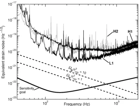
Figure 1 shows reference amplitude spectra of equivalent strain noise, for the three LIGO interferometers during the S1 run. The eventual strain noise goal is also indicated for com-parison. The differences among the three spectra reflect dif-ferences in the operating parameters and hardware imple-mentations of the three instruments; they are in various stages of reaching the final design configuration. For ex-ample, all interferometers operated during S1 at a substan-tially lower effective laser power level than the eventual level of 6 W at the interferometer input; the resulting reduc-tion in signal-to-noise ratio is even greater than the square root of the power reduction, because the detection scheme is designed to be efficient only near the design power level. Thus the shot-noise region of the spectrum共above 200 Hz兲is much higher than the design goal. Other major differences between the S1 state and the final configuration were: par-tially implemented laser frequency and amplitude stabiliza-tion systems; and partially implemented alignment control systems.
Two other important characteristics of the instruments’ performance are the stationarity of the noise, and the duty cycle of operation. The noise was significantly nonstationary, due to the partial stabilization and controls mentioned above. In the frequency band of most importance to this analysis, approximately 60–300 Hz, a factor of 2 variation in the noise amplitude over several hours was typical for the instruments; this is addressed quantitatively in Sec. VI and Fig. 10. As our analysis relies on cross correlating the outputs of two detec-tors, the relevant duty cycle measures are those for double-coincident operation. For the S1 run, the total times of coin-cident science data for the three pairs are: H1-H2, 188 h
共46% duty cycle over the S1 duration兲; H1-L1, 116 h共28%兲; H2-L1, 131 h 共32%兲. A more detailed description of the LIGO interferometers and their performance during the S1 run can be found in Ref.关11兴.
III. STOCHASTIC GRAVITATIONAL WAVE BACKGROUNDS
A. Spectrum
A stochastic background of gravitational radiation is analogous to the cosmic microwave background radiation, though its spectrum is unlikely to be thermal. Sources of a stochastic background could be cosmological or astrophysi-cal in origin. Examples of the former are zero-point fluctua-tions of the space-time metric amplified during inflation, and first-order phase transitions and decaying cosmic string net-works in the early universe. An example of an astrophysical source is the random superposition of many weak signals from binary-star systems. See Refs. 关12兴 and 关13兴for a re-view of sources.
The spectrum of a stochastic background is usually de-scribed by the dimensionless quantity ⍀gw( f ) which is the gravitational-wave energy density per unit logarithmic fre-quency, divided by the critical energy densitycto close the universe:
⍀gw共f兲⬅ f c
dgw
[image:4.612.317.559.56.241.2]d f . 共3.1兲 FIG. 1. Reference sensitivity curves for the three LIGO interfer-ometers during the S1 data run, in terms of equivalent strain noise density. The H1 and H2 spectra are from 9 September 2002, and the L1 spectrum is from 7 September 2002. Also shown are strain spec-tra corresponding to two levels of a stochastic background of gravi-tational radiation defined by Eq.共3.7兲. These can be compared to the expected 90% confidence level upper limits, assuming Gaussian uncorrelated detector noise at the levels shown here, for the inter-ferometer pairs: H2-L1 (⍀0h100
2
⫽10), with 100 h of correlated in-tegration time; H1-H2 (⍀0h100
2 ⫽
0.83), with 150 h of integration time; and H1-L1 (⍀0h100
2 ⫽
The critical densityc⬅3c2H02/8G depends on the present day Hubble expansion rate H0. For convenience we define a dimensionless factor
h100⬅H0/H100, 共3.2兲 where
H100⬅100 km
sec•Mpc⬇3.24⫻10
⫺18 1
sec, 共3.3兲 to account for the different values of H0 that are quoted in the literature.2 Note that ⍀gw( f )h1002 is independent of the actual Hubble expansion rate, so we work with this quantity rather than⍀gw( f ) alone.
Our specific interest is the measurable one-sided power spectrum of the gravitational wave strain Sgw( f ), which is normalized according to:
lim T→⬁ 1 T
冕
⫺T/2T/2
dt兩h共t兲兩2⫽
冕
0⬁
d f Sgw共f兲, 共3.4兲
where h(t) is the strain in a single detector due to the gravi-tational wave signal; h(t) can be expressed in terms of the perturbations hab of the spacetime metric and the detector geometry via:
h共t兲⬅hab共t,xជ0兲 1 2共Xˆ
aXˆb⫺YˆaYˆb兲. 共3.5兲
Here xជ0 specifies the coordinates of the interferometer ver-tex, and Xˆa,Yˆa are unit vectors pointing in the direction of the detector arms. Since the energy density in gravitational waves involves a product of time derivatives of the metric perturbations 共cf. p. 955 of Ref. 关17兴兲, one can show 共see, e.g., Secs. II A and III A in Ref. 关18兴 for more details兲 that Sgw( f ) is related to⍀gw( f ) via:
Sgw共f兲⫽ 3H02 102f
⫺3⍀gw共f兲. 共3.6兲
Thus, for a stochastic gravitational wave background with ⍀gw( f )⬅⍀0⫽const 共as is predicted at LIGO frequencies e.g., by inflationary models in the infinitely slow-roll limit, or by cosmic string models关19兴兲 the power in gravitational waves falls off as 1/f3, with a strain amplitude scale of:
Sgw1/2共f兲⫽5.6⫻10⫺22h100
冑
⍀0冉
100 Hzf
冊
3/2Hz⫺1/2. 共3.7兲
The spectrum ⍀gw( f ) completely specifies the statistical properties of a stochastic background of gravitational radia-tion provided we make several addiradia-tional assumpradia-tions. Here,
we assume that the stochastic background is isotropic, unpo-larized, stationary, and Gaussian. Anisotropic or non-Gaussian backgrounds共e.g., due to an incoherent superposi-tion of gravitasuperposi-tional waves from a large number of unresolved white dwarf binary star systems in our own gal-axy, or a ‘‘popcorn’’ stochastic signal produced by gravita-tional waves from supernova core-collapse events 关20,21兴兲 may require different data analysis techniques from those presented here. 共See, e.g., Refs. 关22,23兴 for discussions of these different techniques.兲
B. Prior observational constraints
While predictions for ⍀gw( f ) from cosmological models can vary over many orders of magnitude, there are several observational results that place interesting upper limits on ⍀gw( f ) in various frequency bands. Table I summarizes these observational constraints and upper limits on the en-ergy density of a stochastic gravitational wave background. The high degree of isotropy observed in the cosmic micro-wave background radiation 共CMBR兲 places a strong con-straint on ⍀gw( f ) at very low frequencies关24兴. Since H100 ⬇3.24⫻10⫺18Hz, this limit applies only over several de-cades of frequency 10⫺18⫺10⫺16Hz which are far below the bands accessible to investigation by either Earth-based (10–104 Hz) or space-based (10⫺4–10⫺1 Hz) detectors.
Another observational constraint comes from nearly two decades of monitoring the time-of-arrival jitter of radio pulses from a number of millisecond pulsars关25兴. These pul-sars are remarkably stable clocks, and the regularity of their pulses places tight constraints on ⍀gw( f ) at frequencies on the order of the inverse of the observation time of the pul-sars, 1/T⬃10⫺8 Hz. Like the constraint derived from the isotropy of the CMBR, the millisecond pulsar timing con-straint applies to an observational frequency band much lower than that probed by Earth-based and space-based de-tectors.
The only constraint on⍀gw( f ) within the frequency band of Earth-based detectors comes from the observed abun-dances of the light elements in the universe, coupled with the standard model of big-bang nucleosynthesis 关26兴. For a nar-row range of key cosmological parameters, this model is in remarkable agreement with the elemental observations. One of the constrained parameters is the expansion rate of the universe at the time of nucleosynthesis, thus constraining the energy density of the universe at that time. This in turn con-strains the energy density in a cosmological background of gravitational radiation 共noncosmological sources of a sto-chastic background, e.g., from a superposition of supernovae signals, are not of course constrained by these observations兲. The observational constraint is on the logarithmic integral over frequency of⍀gw( f ).
All the above constraints were indirectly inferred via elec-tromagnetic observations. There are a few, much weaker constraints on ⍀gw( f ) that have been set by observations with detectors directly sensitive to gravitational waves. The earliest such measurement was made with room-temperature bar detectors, using a split bar technique for wide bandwidth performance 关27兴. Later measurements include an upper
2H0⫽73⫾2⫾7 km/sec/Mpc as shown in Ref.关14兴and from
in-dependent SNIa observations from observatories on the ground 关15兴. The Wilkinson Microwave Anisotropy Probe 1st year 共WMAP1兲observation has H0⫽71⫺⫹3
4
limit from a correlation between the Garching and Glasgow prototype interferometers关28兴, several upper limits from ob-servations with a single cryogenic resonant bar detector 关29,30兴, and most recently an upper limit from observations of two-detector correlations between the Explorer and Nau-tilus cryogenic resonant bar detectors关31,32兴. Note that the cryogenic resonant bar observations are constrained to a very narrow bandwidth (⌬f⬃1Hz) around the resonant frequency of the bar.
IV. DETECTION VIA CROSS CORRELATION
We can express the equivalent strain output si(t) of each of our detectors as:
si共t兲⬅hi共t兲⫹ni共t兲, 共4.1兲 where hi(t) is the strain signal in the ith detector due to a gravitational wave background, and ni(t) is the detector’s equivalent strain noise. If we had only one detector, all we could do would be to put an upper limit on a stochastic background at the detector’s strain noise level; e.g., using L1 we could put a limit of ⍀0h1002 ⬃103 in the band 100–200 Hz. To do much better, we cross correlate the outputs of two detectors, taking advantage of the fact that the sources of noise ni in each detector will, in general, be independent 关12,13,18,33–35兴. We thus compute the general cross correlation:3
Y⬅
冕
⫺T/2 T/2
dt1
冕
⫺T/2 T/2
dt2s1共t1兲Q共t1⫺t2兲s2共t2兲, 共4.2兲
where Q(t1⫺t2) is a 共real兲 filter function, which we will choose to maximize the signal-to-noise ratio of Y. Since the optimal choice of Q(t1⫺t2) falls off rapidly for time delays
兩t1⫺t2兩 large compared to the light travel time d/c between the two detectors,4 and since a typical observation time T will be much, much greater than d/c, we can change the limits on one of the integrations from (⫺T/2,T/2) to (⫺⬁,⬁), and subsequently obtain关18兴:
Y⬇
冕
⫺⬁ ⬁
d f
冕
⫺⬁ ⬁
d f
⬘␦
T共f⫺f⬘兲
˜s1*共f兲Q˜共f⬘兲
˜s2共f⬘
兲, 共4.3兲where
␦T共f兲⬅
冕
⫺T/2 T/2
dte⫺i2f t⫽sin共f T兲
f 共4.4兲
is a finite-time approximation to the Dirac delta function, and ˜si( f ),Q˜ ( f ) denote the Fourier transforms of si(t),Q(t)—i.e., a˜ ( f )⬅兰⫺⬁⬁dte⫺i2f ta(t).
To find the optimal Q˜ ( f ), we assume that the intrinsic detector noise is: 共i兲stationary over a measurement time T; 共ii兲Gaussian; 共iii兲uncorrelated between different detectors; 共iv兲 uncorrelated with the stochastic gravitational wave
sig-3The equations in this section are a summary of Sec. III from Ref.
关18兴. Readers interested in more details and/or derivations of the key equations should refer to Ref. 关18兴 and references contained therein.
4The light travel time d/c between the Hanford and Livingston
[image:6.612.51.564.94.339.2]detectors is approximately 10 msec. TABLE I. Summary of upper limits on⍀0h100
2
over a large range of frequency bands. The upper portion of the table lists indirect limits derived from astrophysical observations. The lower portion of the table lists limits obtained from prior direct gravitational wave measure-ment.
Observational technique
Observed limit
Frequency domain
Comments
Cosmic microwave background ⍀
gw共f兲h100
2 ⭐
10⫺13
冉
10 ⫺16Hz
f
冊
2
3⫻10⫺18⬍f⬍10⫺16Hz 关24兴
Radio pulsar timing ⍀gw( f )h100
2 ⭐
9.3⫻10⫺8 4⫻10⫺9⬍f⬍4⫻10⫺8Hz 95% C.L. bound,关25兴
Big-bang nucleosynthesis 兰f⬎10⫺8Hzd ln f⍀gw( f )h1002 ⭐10⫺5 f⬎10⫺8Hz 95% C.L. bound,关26兴
Interferometers ⍀gw( f )h100
2 ⭐
3⫻105 100ⱗfⱗ1000 Hz Garching-Glasgow关28兴 Room temperature
Resonant bar共correlation兲 ⍀gw( f0)h100
2 ⭐
3000 f0⫽985⫾80 Hz Glasgow关27兴
Cryogenic resonant bar共single兲 ⍀gw( f0)h100
2 ⭐
300 f0⫽907 Hz Explorer关29兴
⍀gw( f0)h100 2
⭐5000 f0⫽1875 Hz ALTAIR关30兴
Cryogenic resonant bar共correlation兲 ⍀gw( f0)h100 2
nal; and共v兲much greater in power at any frequency than the stochastic gravitational wave background. Then the expected value of the cross correlation Y depends only on the stochas-tic signal:
Y⬅
具
Y典
⫽ T2
冕
⫺⬁⬁
d f␥共兩f兩兲Sgw共兩f兩兲Q˜共f兲, 共4.5兲
while the variance of Y is dominated by the noise in the individual detectors:
Y 2⬅
具
共Y⫺
具
Y典
兲2典
⬇T 4冕
⫺⬁⬁
d f P1共兩f兩兲兩Q˜共f兲兩2P2共兩f兩兲. 共4.6兲
Here P1( f ) and P2( f ) are the one-sided strain noise power spectra of the two detectors. The integrand of Eq. 共4.5兲 con-tains a 共real兲 function ␥( f ), called the overlap reduction function关35兴, which characterizes the reduction in sensitivity to a stochastic background arising from the separation time delay and relative orientation of the two detectors. It is a function of only the relative detector geometry 关for coinci-dent and co-aligned detectors, like H1 and H2, ␥( f )⫽1 for all frequencies兴. A plot of the overlap reduction function for correlations between LIGO Livingston and LIGO Hanford is shown in Fig. 2.
From Eqs.共4.5兲and共4.6兲, it is relatively straightforward to show关12兴that the expected signal-to-noise ratio (Y/Y) of Y is maximized when
Q˜共f兲⬀␥共兩f兩兲Sgw共兩f兩兲
P1共兩f兩兲P2共兩f兩兲. 共4.7兲
For the S1 analysis, we specialize to the case ⍀ gw( f )⬅⍀0
⫽const. Then,
Q˜共f兲⫽N ␥共兩f兩兲
兩f兩3P1共兩f兩兲P2共兩f兩兲, 共4.8兲
whereN is a 共real兲overall normalization constant. In prac-tice we choose N so that the expected cross correlation is Y⫽⍀0h100
2
T. For such a choice,
N⫽ 20
2
3H1002
冋
冕
⫺⬁ ⬁d f ␥ 2共兩f兩兲
f6P1共兩f兩兲P2共兩f兩兲
册
⫺1
, 共4.9兲
Y 2⬇
T
冉
10 23H1002
冊
2冋
冕
⫺⬁ ⬁d f ␥ 2共兩f兩兲
f6P1共兩f兲P2共兩f兩兲
册
⫺1
. 共4.10兲
In the sense that Q˜ ( f ) maximizesY/Y, it is the optimal filter for the cross correlation Y. The signal-to-noise ratio Y⬅Y /Y has expected value
具
Y典
⫽ Y Y⬇ 3H0 2
102⍀0
冑
T冋
冕
⫺⬁ ⬁d f ␥ 2共兩f兩兲
f6P1共兩f兩兲P2共兩f兩兲
册
1/2, 共4.11兲
which grows with the square-root of the observation time T, and inversely with the product of the amplitude noise spec-tral densities of the two detectors. In order of magnitude, Eq. 共4.11兲indicates that the upper limit we can place on⍀0h1002 by cross correlation is smaller 共i.e., more constraining兲than that obtainable from one detector by a factor of␥rms
冑
T⌬BW, where⌬BWis the bandwidth over which the integrand of Eq. 共4.11兲 is significant 关roughly the width of the peak of 1/f3Pi( f )], and␥rmsis the rms value of␥( f ) over that band-width. For the LHO-LLO correlations in this analysis, T ⬃2⫻105 sec, ⌬BW⬃100 Hz, and ␥rms⬃0.1, so we expect to be able to set a limit that is a factor of several hundred below the individual detectors’ strain noise,5or ⍀0h1002 ⬃10 as shown in Fig. 1.V. ANALYSIS OF LIGO DATA
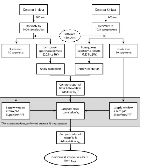
A. Data analysis pipeline
A flow diagram of the data analysis pipeline is shown in Fig. 3 关36兴. We perform the analysis in the frequency do-main, where it is more convenient to construct and apply the optimal filter. Since the data are discretely sampled, we use discrete Fourier transforms and sums over frequency bins rather than integrals. The data ri关k兴 are the raw 共 uncali-brated兲detector outputs at discrete times tk⬅k␦t:
ri关k兴⬅ri共tk兲, 共5.1兲
5More precisely, if the two detectors have unequal strain
sensitivi-ties, the cross-correlation limit will be a factor of␥rms
冑
T⌬BWbe-low the geometric mean of the two noise spectral densities. FIG. 2. Overlap reduction function between the LIGO
Living-ston and the LIGO Hanford sites. The value of兩␥兩 is a little less
[image:7.612.57.295.57.251.2]where k⫽0,1,2, . . . , ␦t is the sampling period, and i labels the detector. We decimate the data to a sampling rate of (␦t)⫺1⫽1024 Hz 共from 16384 Hz兲, since the higher fre-quencies make a negligible contribution to the cross correla-tion. The decimation is performed with a finite impulse re-sponse filter of length 320, and cutoff frequency 512 Hz. The data are split into intervals共labeled by index I) and segments 共labeled by index J) within each interval to deal with detec-tor nonstationarity and to produce sets of cross-correlation values YIJ for which empirical variances can be calculated; see Fig. 4. The time-series data corresponding to the Jth segment in interval I is denoted riIJ关k兴, where k
⫽0,1, . . . ,N⫺1 runs over the total number of samples in the segment.
A single optimal filter Q˜I is calculated and applied for each interval I, the duration of which should be long enough to capture relatively narrow-band features in the power spec-tra, yet short enough to account for significant nonstationary detector noise. Based on observations of detector noise varia-tion, we chose an interval duration of Tint⫽900 sec. The segment duration should be much greater than the light travel time between the two detectors, yet short enough to yield a sufficient number of cross-correlation measurements within each interval to obtain an experimental estimate of the theo-retical varianceY
IJ
2 of the cross correlation statistic Y IJ. We chose a segment duration of Tseg⫽90 sec, yielding ten YIJ values per interval.
To compute the segment cross-correlation values YIJ, the raw decimated data riIJ关k兴are windowed in the time domain 共see Sec. V B for details兲, zero padded to twice their length 共to avoid wrap-around problems 关37兴 when calculating the cross-correlation statistic in the frequency domain兲, and dis-crete Fourier transformed. Explicitly, defining
giIJ关k兴⬅
再
wi关k兴riIJ关k兴 k⫽0, . . . ,N⫺1
0 k⫽N, . . . ,2N⫺1, 共5.2兲 where wi关k兴 is the window function for the ith detector,6the discrete Fourier transform is:
g ˜
iIJ关q兴⬅
兺
k⫽0 2N⫺1␦tgiIJ关k兴e⫺i2kq/2N, 共5.3兲
where N⫽Tseg/␦t⫽92160 is the number of data points in a segment, and q⫽0,1, . . . ,2N⫺1. The cross spectrum g
˜ 1IJ
* 关q兴•g˜2IJ关q兴is formed and binned to the frequency reso-lution,␦f , of the optimal filter Q˜I:7
GIJ关ᐉ兴⬅ 1
nb q⫽n
兺
bᐉ⫺m nbᐉ⫹mg ˜
1IJ
* 关q兴˜g2IJ关q兴, 共5.4兲
where ᐉmin⭐ᐉ⭐ᐉmax,nb⫽2Tseg␦f is the number of fre-quency values being binned, and m⫽(nb⫺1)/2. The indexᐉ labels the discrete frequencies, fᐉ⬅ᐉ␦f . The GIJ关ᐉ兴 are computed for a range of ᐉ that includes only the frequency band that yields most of the expected signal-to-noise ratio 共e.g., 40–314 Hz for the LHO-LLO correlations兲, as de-scribed in Sec. V C. The cross-correlation values are calcu-lated as:
YIJ⬅2 Re
冋
兺
ᐉ⫽ᐉmin
ᐉmax
␦f Q˜I关ᐉ兴GIJ关ᐉ兴
册
. 共5.5兲6In general, one can use different window functions for different
detectors. However, for the S1 analysis, we took w1关k兴⫽w2关k兴. 7As discussed below,␦f⫽0.25 Hz yielding n
b⫽45 and m⫽22.
[image:8.612.55.296.51.335.2]FIG. 3. Data analysis flow diagram for the stochastic search. The raw detector signal共i.e., the uncalibrated differential arm error signal兲is fed into the pipeline in 900-sec-long intervals. Simulated stochastic background signals can be injected near the beginning of each data path, allowing us to test the data analysis routines in the presence of known correlations.
FIG. 4. Time-series data from each interferometer is split into M
900-sec intervals, which are further subdivided into n⫽10 90-sec
data segments. Cross-correlation values YIJare calculated for each
90-sec segment; theoretical variances YIJ
2
are calculated for each
900-sec interval. Here I⫽1,2, . . . , M labels the different intervals,
and J⫽1,2, . . . ,n labels the individual segments within each
Some of the frequency bins within the兵ᐉmin,ᐉmax其 range are excluded from the above sum to avoid narrow-band instru-mental correlations, as described in Sec. V C. Except for the details of windowing, binning, and band-limiting, Eq. 共5.5兲 for YIJ is just a discrete-frequency approximation to Eq. 共4.3兲for Y for the continuous-frequency data, with d f
⬘␦
T( f⫺f
⬘
) approximated by a Kronecker delta ␦ᐉᐉ⬘ in discrete frequencies fᐉ and fᐉ⬘.8In calculating the optimal filter, we estimate the strain noise power spectra PiI for the interval I using Welch’s method: 449 periodograms are formed and averaged from 4096-point, Hann-windowed data segments, overlapped by 50%, giving a frequency resolution ␦f⫽0.25 Hz. To cali-brate the spectra in strain, we apply the calibration response function R˜i( f ) which converts the raw data to equivalent strain: s˜i( f )⫽R˜i⫺1( f )r˜i( f ). The calibration lines described in Sec. II were measured once per 60 sec; for each interval I, we apply the response function, R˜iI, corresponding to the middle 60 sec of the interval. The optimal filter Q˜I for the case⍀gw( f )⬅⍀0⫽const is then constructed as:
Q˜I关ᐉ兴⬅NI
␥关ᐉ兴
兩fᐉ兩3共R˜1I关ᐉ兴P1I关ᐉ兴兲*共R˜2I关ᐉ兴P2I关ᐉ兴兲, 共5.6兲
where␥关ᐉ兴⬅␥( fᐉ), and R˜iI关ᐉ兴⬅R˜iI( fᐉ). By including the additional response function factors R˜iI in Eq. 共5.6兲, Q˜I has the appropriate units to act directly on the raw detector out-puts in the calculation of YIJ 关cf. Eq.共5.5兲兴.
The normalization factor NI in Eq. 共5.6兲 takes into ac-count the effect of windowing关38兴. ChoosingNI so that the theoretical mean of the cross correlation YIJ is equal to ⍀0h1002 Tseg for all I,J 共as was done for Y in Sec. IV兲, we have:
NI⫽ 202 3H1002
1 w1w2
冋
2
兺
ᐉ⫽ᐉmin
ᐉmax
␦f ␥
2关ᐉ兴
fᐉ6P1I关ᐉ兴P2I关ᐉ兴
册
⫺1 ,
共5.7兲
YIJ 2 ⫽T
seg
冉
102 3H1002冊
2 w12w22
共w1w2兲2
⫻
冋
2兺
ᐉ⫽ᐉmin
ᐉmax
␦f ␥
2关ᐉ兴
fᐉ6P1I关ᐉ兴P2I关ᐉ兴
册
⫺1
, 共5.8兲
where
w1w2⬅ 1 N k
兺
⫽0N⫺1
w1关k兴w2关k兴, 共5.9兲
w12w22⬅1 N k
兺
⫽0N⫺1
w12关k兴w22关k兴, 共5.10兲
provided the windowing is sufficient to prevent significant leakage of power across the frequency band 共see Sec. V B and Ref.关38兴for more details兲. Note that the theoretical vari-ance Y
IJ
2
depends only on the interval I, since the cross correlations YIJ have the same statistical properties for each segment J in I.
For each interval I, we calculate the mean, YI, and 共sample兲standard deviation, sYIJ, of the 10 cross-correlation values YIJ:
YI⬅ 1 10J
兺
⫽110
YIJ, 共5.11兲
sY
IJ⬅
冑
1 9 J
兺
⫽110
共YIJ⫺YI兲2. 共5.12兲
We also form a weighted average, Yopt, of the YI over the whole run:
Yopt⬅
兺
I YIJ⫺2 YI
兺
I YIJ⫺2
. 共5.13兲
The statistic Yopt maximizes the expected signal-to-noise ra-tio for a stochastic signal, allowing for nonstara-tionary detector noise from one 900-sec interval I to the next 关18兴. Dividing Yopt by the time Tseg over which an individual cross-correlation measurement is made gives, in the absence of cross-correlated detector noise, an estimate of the stochastic background level:9 ⍀ˆ0h100
2 ⫽Y
opt/Tseg.
Finally, in Sec. V E we will be interested in the spectral properties of YIJ, YI, and Yopt. Thus, for later reference, we define:
Y ˜
IJ关ᐉ兴⬅Q˜I关ᐉ兴GIJ关ᐉ兴, 共5.14兲
Y ˜
I关ᐉ兴⬅ 1 10J
兺
⫽110 Y ˜
IJ关ᐉ兴, 共5.15兲
Y
˜opt关ᐉ兴⬅
兺
I Y⫺IJ2 Y ˜I关ᐉ兴
兺
I YIJ⫺2
. 共5.16兲
Note that 2 Re兺ᐉ⫽ᐉ
min
ᐉmax ␦f• of the above quantities equal
YIJ, YI, and Yopt, respectively.
8
To make this correspondence with Eq.共4.3兲, the factor of 2 and real part in Eq.共5.5兲are needed since we are summing only over positive frequencies, e.g., 40–314 Hz for the LHO-LLO correlation. Basically, integrals over continuous frequency are replaced by sums over discrete frequency bins using the correspondence 兰⫺⬁⬁ d f
→2 Re兺ᐉ⫽ᐉ min
ᐉmax ␦f .
9We use a hat ˆ to indicate an estimate of the actual 共unknown兲
B. Windowing
In taking the discrete Fourier transform of the raw 90-sec data segments, care must be taken to limit the spectral leak-age of large, low-frequency components into the sensitive band. In general, some combination of high-pass filtering in the time domain, and windowing prior to the Fourier trans-form can be used to deal with spectral leakage. In this analy-sis we have found it sufficient to apply an appropriate win-dow to the data.
Examining the dynamic range of the data helps establish the allowed leakage. Figure 1 shows that the lowest instru-ment noise around 60 Hz is approximately 10⫺19/
冑
Hz 共for L1兲. While not shown in this plot, the rms level of the raw data corresponds to a strain of order 10⫺16, and is due to fluctuations in the 10–30-Hz band. Leakage of these low-frequency components must be at least below the sensitive band noise level; e.g., leakage must be below 10⫺3 for a 30-Hz offset. A tighter constraint on the leakage comes when considering that these low-frequency components may be correlated between the two detectors, as they surely will be at some frequencies for the two interferometers at LHO, due to the common seismic environment. In this case the leakage should be below the predicted stochastic background sensi-tivity level, which is approximately 2.5 orders of magnitude below the individual detector noise levels for the LHO H1-H2 case. Thus, the leakage should be below 3⫻10⫺6for a 30-Hz offset.On the other hand, we prefer not to use a window that has an average value significantly less than unity 共and corre-spondingly low leakage, such as a Hann window兲, because it will effectively reduce the amount of data contributing to the cross correlation. Provided that the windowing is sufficient to prevent significant leakage of power across the frequency range, the net effect is to multiply the expected value of the signal-to-noise ratio by w1w2/
冑
w12w22 关cf. Eqs.共5.7兲,共5.8兲兴. For example, when w1 and w2 are both Hann windows, this factor is equal to冑
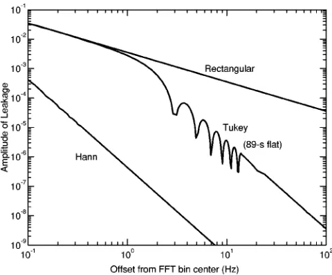
18/35⬇0.717, which is equivalent to reducing the data set length by a factor of 2. In principle one should be able to use overlapping data segments to avoid this effective loss of data, as in Welch’s power spectrum estima-tion method. In this case, the calculaestima-tions for the expected mean and variance of the cross correlations would have to take into account the statistical interdependence of the over-lapping data.Instead, we have used a Tukey window 关39兴, which is essentially a Hann window split in half, with a constant sec-tion of all 1’s in the middle. We can choose the length of the Hann portion of the window to provide sufficiently low leak-age, yet maintain a unity value over most of the window. Figure 5 shows the leakage function of the Tukey window that we use共a 1-sec Hann window with an 89-sec flat section spliced into the middle兲, and compares it to Hann and rect-angular windows. The Tukey window leakage is less than 10⫺7 for all frequencies greater than 35 Hz away from the FFT bin center. This is 4 orders of magnitude better than what is needed for the LHO-LLO correlations and a factor of 30 better suppression than needed for the H1-H2 correlation.
To explicitly verify that the Tukey window behaved as expected, we re-analyzed the H1-H2 data with a pure Hann window 共see also Sec. VIII兲. The result of this re-analysis, properly scaled to take into account the effective reduction in observation time, was, within error, the same as the original analysis with a Tukey window. Since the H1-H2 correlation is the most prone of all correlations to spectral leakage共due to the likelihood of cross-correlated low-frequency noise components兲, the lack of a significant difference between the pure Hann and Tukey window analyses provided additional support for the use of the Tukey window.
C. Frequency band selection and discrete frequency elimination
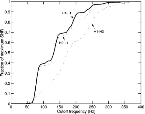
[image:10.612.317.557.56.255.2]In computing the discrete cross-correlation integral, we are free to restrict the sum to a chosen frequency region or regions; in this way the variance can be reduced 共e.g., by excluding low frequencies where the detector power spectra are large and relatively less stationary兲, while still retaining most of the signal. We choose the frequency ranges by de-termining the band that contributes most of the expected signal-to-noise ratio, according to Eq.共4.11兲. Using the strain power spectra shown in Fig. 1, we compute the signal-to-noise ratio integral of Eq.共4.11兲from a very low frequency 共a few Hz兲 up to a variable cutoff frequency, and plot the resulting signal-to-noise ratio versus cutoff frequency 共Fig. 6兲. For each interferometer pair, the lower band edge is cho-sen to be 40 Hz, while the upper band edge choices are 314 Hz for LHO-LLO correlations共where there is a zero in the overlap reduction function兲, and 300 Hz for H1-H2 correla-tions 共chosen to exclude ⬃340-Hz resonances in the test mass mechanical suspensions, which were not well resolved in the power spectra兲.
Within the 40–314 共300兲-Hz band, discrete frequency bins at which there are known or potential instrumental cor-relations due to common periodic sources are eliminated from the cross-correlation sum. For example, a significant feature in all interferometer outputs is a set of spectral lines extending out to beyond 2 kHz, corresponding to the 60-Hz power line and its harmonics (n60-Hz lines兲. Since these lines obviously have a common source—the mains power supplying the instrumentation—they are potentially lated between detectors. To avoid including any such corre-lation in the analysis, we eliminate the n60-Hz frequency bins from the sum in Eq. 共5.5兲.
Another common periodic signal arises from the data ac-quisition timing systems in the detectors. The absolute tim-ing and synchronization of the data acquisition systems be-tween detectors is based on 1 pulse-per-second signals produced by Global Positioning System 共GPS兲 receivers at each site. In each detector, data samples are stored tempo-rarily in 1/16-sec buffers, prior to being collected and written to disk. The process, through mechanisms not yet estab-lished, results in some power at 16 Hz and harmonics in the detectors’ output data channels. These signals are extremely narrow band and, due to the stability and common source of the GPS-derived timing, can be correlated between detectors. To avoid including any of these narrow-band correlations, we eliminate the n16-Hz frequency bins from the sum in Eq. 共5.5兲.
Finally, there may be additional correlated narrow-band features due to highly stable clocks or oscillators that are common components among the detectors 共e.g., computer monitors can have very stable sync rates, typically at 70 Hz兲. To describe how we avoid such features, we first present a quantitative analysis of the effect of coherent spectral lines on our cross-correlation measurement. We begin by follow-ing the treatment of correlated detector noise given in Sec. V E of Ref.关18兴. The contribution of cross-correlated
detec-tor noise to the cross correlation Y will be small compared to the intrinsic measurement noise if
冏
T 2冕
⫺⬁⬁
d f P12(兩f兩)Q˜共f兲
冏
ⰆY, 共5.17兲where P12(兩f兩) is the cross-power spectrum of the strain noise (n1,n2) in the two detectors, T is the total observation time, and Y is defined by Eq. 共4.6兲. Using Eq. 共4.8兲, this condition becomes
N
冏
冕
⫺⬁⬁
d f P12共兩f兩兲␥共兩f兩兲
兩f兩3P1共兩f兩兲P2共兩f兩兲冏Ⰶ 2Y
T , 共5.18兲
or, equivalently, 3H1002
52
冏
冕
⫺⬁ ⬁d f P12共兩f兩兲␥共兩f兩兲
兩f兩3P1共兩f兩兲P2共兩f兩兲冏Ⰶ2Y
⫺1, 共5.19兲
where Eqs. 共4.9兲,共4.10兲 were used to eliminate N in terms of Y2:
N⫽3H100 2
52 Y
2
T . 共5.20兲
Now consider the presence of a correlated periodic signal, such that the cross spectrum P12( f ) is significant only at a single共positive兲discrete frequency, fL. For this component to have a small effect, the above condition becomes:
3H1002 52
冏
⌬fP12共fL兲␥共fL兲
fL3P1共fL兲P2共fL兲
冏
ⰆY⫺
1, 共5.21兲
where⌬f is the frequency resolution of the discrete Fourier transform used to approximate the frequency integrals. The left-hand-side of Eq.共5.21兲can be expressed in terms of the coherence function⌫12( f ), which is essentially a normalized cross spectrum, defined as关40兴:
⌫12共f兲⬅ 兩P12共f兲兩 2
P1共f兲P2共f兲. 共5.22兲 The condition on the coherence at fL is thus
关⌫12共fL兲兴1/2Ⰶ Y⫺
1
⌬f 52 3H1002
冑
P1共fL兲P2共fL兲兩fL⫺3␥共fL兲兩
. 共5.23兲
Since Y increases as T1/2, the limit on the coherence ⌫12( fL) becomes smaller as 1/T. To show how this condition applies to the S1 data, we estimate the factors in Eq. 共5.23兲 for the H2-L1 pair, focusing on the band 100–150 Hz. We assume any correlated spectral line is weak enough that it does not appear in the power spectrum estimates used to construct the optimal filter. Noting that the combination (3H1002 /102) f⫺3 is just the power spectrum of gravitational waves Sgw( f ) with⍀0h100
2 ⫽
1 关cf. Eq.共3.6兲兴, we can evalu-ate the right-hand side of Eq.共5.23兲by estimating the ratios 关Pi/Sgw兴1/2 from Fig. 1 for ⍀0h
100
[image:11.612.54.296.58.249.2]2 ⫽1. Within the band FIG. 6. Curves show the fraction of maximum expected
signal-to-noise ratio as a function of cutoff frequency, for the three inter-ferometer pairs. The curves were made by numerically integrating
Eq.共4.11兲from a few Hz up to the variable cutoff frequency, using
100–150 Hz, this gives: ( P1P2)1/2/Sgwⲏ2500. The overlap reduction function in this band is兩␥兩ⱗ0.05. The appropriate frequency resolution ⌬f is that corresponding to the 90-sec segment discrete Fourier transforms, so ⌬f⫽0.011 Hz. As described later in Sec. VI, we calculate a statistical error, ⍀, associated with the stochastic background estimate
Yopt/Tseg. Under the implicit assumption made in Eq.共5.23兲 that the detector noise is stationary, one can show that Y
⫽T⍀. Finally, referring to Table IV for an estimate of⍀, and using the total H2-L1 observation time of 51 h, we ob-tainY⬇2.8⫻106 sec. Thus, the condition of Eq.共5.23兲 be-comes: 关⌫12( fL)兴1/2Ⰶ1.
Using this example estimate as a guide, specific lines are rejected by calculating the coherence function between de-tector pairs for the full sets of analyzed S1 data, and elimi-nating any frequency bins at which ⌫12( fL)⭓10⫺2. The co-herence functions are calculated with a frequency resolution of 0.033 Hz, and approximately 20 000共35 000兲averages for the LHO-LLO 共LHO-LHO兲 pairs, corresponding to statisti-cal uncertainty levels ⌫⬅1/Navg of approximately 5
⫻10⫺5 (3⫻10⫺5). The exclusion threshold thus corre-sponds to a cut on the coherence data of order 100 ⌫.
For the H2-L1 pair, this procedure results in eliminating the 250-Hz frequency bin, whose coherence level was about 0.02; the H2-L1 coherence function over the analysis band is shown in Fig. 7. For H1-H2, the bins at 168.25 Hz and 168.5 Hz were eliminated, where the coherence was also about 0.02 共see Fig. 17兲. The sources of these lines are unknown. For H1-L1, no additional frequencies were removed by the coherence threshold 共see Fig. 8兲.
It is worth noting that correlations at the n60-Hz lines are suppressed even without explicitly eliminating these fre-quency bins from the sum. This is because these frequencies have a high signal-to-noise ratio in the power spectrum esti-mates, and thus they have relatively small values in the op-timal filter. The opop-timal filter thus tends to suppress spectral lines that show up in the power spectra. This effect is illus-trated in Fig. 9, and is essentially the result of having four powers of s˜i( f ) in the denominator of the integrand of the cross correlation, but only two powers in the numerator. Nonetheless, we chose to remove the n60-Hz bins from the cross-correlation sum for robustness, and as good practice for future analyses, where improvements in the electronics instrumentation may reduce the power line coupling such that the optimal filter suppression is insufficient.
Such optimal filter suppression does not occur, however, for the 16-Hz line and its harmonics, and the additional 168.25-, 168.5-, 250-Hz lines; these lines typically do not appear in the power spectrum estimates, or do so only with a small signal-to-noise ratio. These lines must be explicitly eliminated from the cross-correlation sum. These discrete frequency bins are all zeroed out in the optimal filter, so that each excluded frequency removes 0.25 Hz of bandwidth from the calculation.
D. Results and interpretation
The primary goal of our analysis is to set an upper limit on the strength of a stochastic gravitational wave
[image:12.612.319.560.55.389.2]back-ground. The cross-correlation measurement is, in principle, sensitive to a combination of a stochastic gravitational back-ground and instrumental noise that is correlated between two detectors. In order to place an upper limit on a gravitational wave background, we must have confidence that instrumen-tal correlations are not playing a significant role. Gaining such confidence for the correlation of the two LHO interfer-ometers may be difficult, in general, as they are both exposed to many of the same environmental disturbances. In fact, for the S1 analysis, a strong共negative兲correlation was observed between the two Hanford interferometers, thus preventing us from setting an upper limit on⍀0h1002 using the H1-H2 pair results. The correlated instrumental noise sources, relatively broadband compared to the excised narrow-band features de-scribed in the previous section, produced a significant H1-H2 cross correlation 共signal-to-noise ratio of ⫺8.8); see Sec. VIII for further discussion of the H1-H2 instrumental corre-lations.
FIG. 7. Coherence between the H2 and L1 detector outputs dur-ing S1. The coherence is calculated with a frequency resolution of
0.033 Hz and Navg⬇20 000 periodogram averages共50% overlap兲;
Hann windows are used in the Fourier transforms. There are
sig-nificant peaks at harmonics of 16 Hz共data acquisition buffer rate兲
and at 250 Hz共unknown origin兲. These frequencies are all excluded
from the cross-correlation sum. The broadband coherence level
cor-responds to the expected statistical uncertainty level of 1/Navg⬇5
On the other hand, for the widely separated 共LHO-LLO兲 interferometer pairs, there are only a few paths through which instrumental correlations could arise. Narrow-band inter-site correlations are seen, as described in the previous section, but the described measures have been taken to ex-clude them from the analysis. Seismic and acoustic noise in the several to tens of Hz band have characteristic coherence lengths of tens of meters or less, compared to the 3000-km LHO-LLO separation, and pose little problem. Globally cor-related magnetic field fluctuations have been identified in the past as the most likely candidate capable of producing broad-band correlated noise in the widely separated detectors关34兴. An order-of-magnitude analysis of this effect was made in Ref.关18兴, concluding that correlated field fluctuations during magnetically noisy periods 共such as during thunderstorms兲 could produce a LHO-LLO correlated strain signal corre-sponding to a stochastic gravitational background⍀0h1002 of order 10⫺8. These estimates evaluated the forces produced on the test masses by the correlated magnetic fields, via mag-nets that are bonded to the test masses to provide position
and orientation control.10 Direct tests made on the LIGO interferometers indicate that the magnetic field coupling to the strain signal was generally much higher during S1—up to 102 times greater for a single interferometer—than these force coupling estimates. Nonetheless, the correspondingly modified estimate of the equivalent⍀due to correlated mag-netic fields is still 5 orders of magnitude below our present sensitivity. Indeed, Figs. 7 and 8 show no evidence of any significant broadband instrumental correlations in the S1 data. We thus set upper limits on⍀0h1002 for both the H1-L1 and the H2-L1 pair results.
Accounting for the combination of a gravitational wave background and instrumental correlations, we define an ef-fective ⍀, denoted ⍀eff, for which our measurement Yopt/Tsegprovides an estimate:
⍀ˆ effh100
2 ⬅
Yopt/Tseg⫽共⍀ˆ0⫹⍀ˆinst兲h100 2
. 共5.24兲
Note that ⍀inst 共associated with instrumental correlations兲 may be either positive or negative, while⍀0for the gravita-tional wave background must be non-negative. We calculate a standard two-sided, frequentist 90% confidence interval on ⍀effh1002 as follows:
关⍀ˆeffh 100 2 ⫺1.65ˆ
⍀,tot,⍀ˆeffh100 2 ⫹1.65ˆ
⍀,tot兴 共5.25兲
where ˆ⍀,tot is the total estimated error of the cross-correlation measurement, as explained in Sec. VI. In a
fre-10The actual limit on⍀ 0h100
2
that appears in Ref.关18兴 is 10⫺7,
[image:13.612.59.296.55.379.2]since the authors assumed a magnetic dipole moment of the test mass magnets that is a factor of 10 higher than what is actually used.
FIG. 8. Coherence between the H1 and L1 detector outputs dur-ing S1, calculated as described in the caption of Fig. 7. There are
significant peaks at harmonics of 16 Hz 共data acquisition buffer
rate兲. These frequencies are excluded from the cross-correlation
sum. The broadband coherence level corresponds to the expected
[image:13.612.320.556.57.239.2]statistical uncertainty level of 1/Navg⬇5⫻10⫺5.