Performance comparison of heating control strategies combining simulation and experimental results

PERFORMANCE COMPARISON OF HEATING CONTROL STRATEGIES

COMBINING SIMULATION AND EXPERIMENTAL RESULTS

Michaël Kummert

, Philippe André

, and Athanassios A. Argiriou

_{École Polytechnique de Montréal, Dépt. de Génie Mécanique}

Case Postale 6079, succursale Centre-Ville, Montréal, QC H3C 3A7, Canada

michael.kummert

polymtl.ca

2

_{Université de Liège, Dépt. des Sciences et Gestion de l'Environnement – Arlon, Belgium}

_{University of Patras, Dept. of Physics – Patras, Greece}

ABSTRACT

Different heating system controllers for passive solar buildings are compared on two different buildings. The performance criterion combines energy performance and thermal comfort using the "cost function" paradigm. The experimental facilities did not allow a direct experimental comparison by using two identical buildings.

The controllers were implemented alternatively in one building and a performance comparison was obtained in two ways: first by identifying short periods that have similar driving variables (weather conditions and building occupancy) and comparing the experimental results obtained in both cases. The second method mixes experiments and simulation using a well-tuned model of the building and its occupants.

This paper discusses the results obtained using the above methods and shows that both methods give consistent estimates of the difference between controllers, while the second method allows to extrapolate useful information from the limited data available.

INTRODUCTION

The problem of heating control in passive solar buildings, or in modern, well-insulated buildings with substantial thermal mass (or heat capacity) and high internal and/or solar gains, is characterized by a need of anticipation and by the variety of time constants involved (Kummert, 2001).

The need for anticipation arises in part from the well-known optimal start problem, where the controller attempts to start heating as late as possible in order to save energy. This problem is reinforced by the high thermal inertia typically present in passive solar buildings.

On the other hand, passive solar buildings are also subject to afternoon overheating: during the mid-season, it is frequent to have a need for heating in the morning while the accumulation of solar energy throughout the day leads to overheating in the afternoon. An intelligent controller can prevent this by slightly under-heating the building in the

morning. This usually requires a rather long anticipation horizon.

Those observations formed the basis of a joint research project to develop advanced controllers especially designed for passive solar buildings. Different control algorithms were compared in simulation and during experimental tests on two different buildings (Christoffers et al., 2000). This paper is centered on the controllers that were tested for the longest periods in two experimental buildings.

Experimental comparison of different controllers

HVAC control studies that compare the performance of different controllers are usually performed in simulation (e.g. Zaheer-Uddin, 1992 and van Schijndel, 2002). When an experimental validation is part of the study, most authors have benefited from two identical buildings or two identical reference zones in a building (Nygard-Fergusson, 1990). The experimental facilities that were available for this project did not include identical reference zones or identical buildings. A method had to be developed in order to obtain a performance comparison between different control algorithms.

Kolokotsa (2003) presents a study where 4 controllers are compared in simulation and the best performer is implemented for experimental validation. While this is an interesting option, the results presented here below will show that a model validated with one control strategy might not be able to simulate the performance of very different controllers accurately. In (Oestreicher, 1996), the experimental results of two controllers rotated in the same building are compared based on their ability to use free gains to save heating energy.

The optimal controller

The optimal controller that was compared to reference solutions in the present study allows to realize a real compromise between energy and comfort, thanks to a cost function that is a weighted sum of the energy consumption (again expressed in terms of Joules, money, or tons of CO2) and the

discomfort in the building. This implies that the performance criterion used in the comparison must take those two aspects into account. A similar cost function is used in (Mozer et al, 1997) to assess the performance of an optimal controller based on an Artificial Neural Network.

PERFORMANCE CRITERION

The "cost function"

The notion of cost function is used in the optimal controller. The cost function must be an expression of the trade-off between comfort and energy consumption.

The energy cost is considered to be proportional to the energy consumption. The multiplier can be time-varying and can represent financial or environmental costs.

The chosen indicator of thermal (dis)comfort is Fanger's PPD (Predictive Percentage of Dissatisfied – Fanger, 1972).

Assessing the discomfort cost

In the discomfort cost, PPD is computed with default parameters for non-measured aspects (air velocity, humidity and metabolic activity). Furthermore, it is assumed that occupants can adapt their clothing to the zone temperature. This method allows modeling a comfort range in which occupants are satisfied. With the chosen value for parameters, the comfort zone covers operative temperatures from 21°C to 24°C. The PPD is also shifted down by 5%, to give a minimum value of 0. This modified PPD index will be referred to as PPD'. This gives, respectively for discomfort cost and energy cost (Jd and Je):

(

)

d

J =

∫

e b

J =

∫

The global cost (J) is a weighted sum of Jd and Je:

d e

J= αJ +J (3)

The role of the α parameter is to give more or less importance to comfort with respect to energy. It can be seen as a "comfort setting" of the controller. If a user increases the value of α, she/he is actually saying that comfort should have more importance in the trade-off that is made to control the HVAC plant.

If we assume that the energy cost is expressed in kWh, the units of α will be [kW %PPD'-1_].

In other words, α is the energy quantity (expressed in kWh or in terms of environmental impact, financial cost, etc.) which may be used to reduce the Predicted Percentage of Dissatisfied occupants by 1% during 1 hour.

Performance comparison

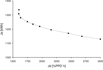
Each value of the weighting factor α will lead to a different solution of the optimization problem. If the performance over a given period (e.g. one month, or a full heating season) is considered, the performance of a controller can be represented by a total value of Jd and Je, or a point in the (Jd, Je) plane.

The solutions obtained by the same controller for different settings (e.g. different weighting factors for an optimal controller based on the cost function described here above) is a trajectory in the (Jd, Je)

plane.

This is illustrated in Figure 1. While such a "controller trajectory" is easily obtained in simulation, it is important to realize that experimental results for the entire period that is selected will lead to one point in the (Jd, Je).plane

1000 1100 1200 1300 1400

1500 1750 2000 2250 2500 2750 3000

Jd [%PPD' h]

Je

[kW

h

]

Figure 1: Typical controller performance for different settings. Costs are summed over a given period. Experimental data for that period would yield only 1 point

EXPERIMENTAL BUILDINGS

The experimental tests were carried on two very different buildings:

• The "Academic Building" of the Environmental sciences and Management campus of the University of Liège, in Belgium (Arlon). This occupied building has a heavy masonry structure and the South wall is protected by a glazed skin. Two administrative offices were selected as the reference zone. The building has a hydronic heating system with radiators and the optimal controller acts on the system through the water supply temperature.

• The PASSYS test cell maintained by the National Observatory of Athens, in Greece (Van Dijk, 1994). The unoccupied test cell has one fully instrumented reference zone. It has a lightweight wooden structure and an electric heating controlled through an ON/OFF switch.

The contrasts between both buildings allowed to test the controllers in very different environments, as well as to validate the comparison methodology in different contexts.

RESULTS IN AN OCCUPIED PASSIVE

SOLAR BUILDING

Controllers

The Conventional controller (Conv), which was

used in the building before this study, implements a conventional "heating curve + thermostatic valves" strategy. The water supply temperature is controlled by a heating curve varying according to a fixed schedule (Day-Night). The heating curve is designed to maintain 21°C during day and 15°C during night (or weekends). Each radiator is equipped with a thermostatic valve that can be adjusted by building occupants.

The "Reference" controller (Ref) is a PID acting on

the water supply temperature to maintain the desired setpoint in the reference zone, where thermostatic valves are removed. Other rooms are still equipped with thermostatic valves. Compared with the reference controller, this one has a better thermostatic control in the reference zone and a more efficient night setback.

The optimal controller (Opt) is a model-based

predictive controller (Kummert, 2001). The optimization algorithm uses an internal simplified model of the building and the hydronic heating system to simulate future control sequences with a forecasting horizon that ranges from 6 to 24 hours. Occupancy is forecast based on a fixed schedule and the weather forecasts are obtained via email from the

national weather institute. The optimal control sequence is selected to minimize a performance criterion which is a linear-quadratic approximation of (3). The controller uses a receding horizon, i.e. the optimization is repeated with a period shorter than the forecasting horizon (Typically 1 to 3 hours). The model parameters are identified online in order to compensate for modeling errors and system changes (e.g. windows opened by occupants). The control algorithm is described in more details in another paper presented at this conference (Kummert and André, 2005).

Available data sets

The available data cover 2 heating seasons, and 170 days are available after removing missing and dubious data. The 3 controllers were implemented alternatively but their historical succession causes significant discrepancies in the weather data, as shown in Table 1. The building has a very high thermal mass, so one full week of "transition" was allowed once a new controller was implemented.

Table 1: Weather data statistics for the data sets

Variable Conv Ref Opt

Tamb,min[°C] -4.1 -4.1 -8.3

Tamb,max [°C] 18.7 9.3 17.2

Tamb,avg[°C] 5.4 2.1 3.8

ATavg[°C] 6.6 4.1 5.2

HSmin [MJ m-2] 0.7 0.1 0.1

HSmax [MJ m-2] 18.6 9.5 14.4

HSavg [MJ m-2] 7.4 2.0 3.5

This table shows slightly different characteristics for the temperature, but a significant difference in mean solar radiation between the 3 periods: the sunshine was higher when the Conventional controller was tested. In a passive solar building, this has a string effect on the heating load, but more importantly a dramatic effect on comfort cost since the most significant uncomfortable episodes are actually due to afternoon overheating (underheating can be reduced by changing the settings of the controller, such as thermostatic valves setpoint or heating start time).

Comparison on short periods

Table 2: Weather data statistics and measured controller performance for 2 short periods

Variable Conv Opt

Tamb,min [°C] 2.0 3.5

Tamb,max [°C] 18.7 17.2

Tamb,avg [°C] 10.0 9.3

HSavg [MJ m-2] 81 75

Je [MJ] 212 184

Jd,max [%PPD'] 67 62

Jd,avg [%PPD'] 3.8 2.4

PMVmin [-] 0.25 0.07

PMVmax [-] -0.13 -0.34

PMVavg [-] 0.43 0

The Conventional controller uses a fixed schedule. During relatively warm periods, this schedule is too conservative, which leads to wasted energy to pre-heat the building too long in advance. Furthermore, such a warm building is more subject to overheating. This last point is still reinforced by the proportional band of the thermostatic valves, which reduce the power when the temperature reaches the setpoint but do not really stop heating until the temperature is about 0.5 °C above this setpoint.

In this kind of situation, the optimal controller is able to reduce the energy consumption while reducing discomfort. Energy savings on the considered period reach 13%, for a significantly reduced discomfort ("optimal" discomfort cost is 28% from "conventional" cost).

Another example is given in Table 3, where data sets for the Reference controller and the Optimal controller.

Table 3: Weather data statistics and measured controller performance for 2 short periods(2)

Variable Ref Opt

Tamb,min [°C] -4.1 -8.3

Tamb,max [°C] 9.1 8.2

Tamb,avg [°C] 1.1 1.3

HSavg [MJ m-2] 32 31

Je [MJ] 487 431

Jd,max [%PPD'] 6.1 3.1

Jd,avg [%PPD'] 0.25 0.14

PMVmin [-] -0.55 -0.39

PMVmax [-] 0 0

PMVavg [-] -0.04 -0.03

During this cold period, the fixed schedule leads to energy waste on some days because the pre-heating time is too long, but to high discomfort on other days because the pre-heating time is too short. The optimal controller sometimes underestimates the pre-heating time as well, leading to relatively high

discomfort, but it adapts this pre-heating time to the building state. Over the whole period, once again this allows to reduce the discomfort while saving energy (about 12% energy savings with 44% discomfort cost reduction).

Comparison using simulation: principle

The results from comparisons on short periods show that the relative performance of different controllers is strongly affected by the weather. A comparison entirely based on experimental results would therefore need to include the different typical conditions (cold and cloudy, cold and sunny, etc.) and use the appropriate weighting factors.

Another approach to obtain a performance comparison on a typical year is outlined here below:

• During a first period, the controller one is tested on the building

• During a second period, the controller two is tested on the building

• The experimental results are used to tune and validate a building model adapted to the experimental circumstances, which can be checked by the simulated performance of controller one on the first period and the simulated performance of controller two during the second period

• Finally, the performance of controller one during the second period and the performance of controller two during the first period are simulated. A virtual comparison can then be performed over the same periods

Tuning the building model

Parameter identification on a detailed building is a complex problem, due to the large number of parameters and to the possibility of achieving the same result through different actions (e.g. increase the infiltration rate or increase the thermal conductivity of a low-mass wall or window).

In the case of an occupied building where occupants can take actions (e.g. open windows), the model also needs to reproduce the occupants’ behavior rather than its effects.

identified and used when simulating a different controller, the results would most likely be incorrect because a different controller would induce a different temperature in the room, hence a different action from the occupants. It is the reaction of occupants to temperature that must be fitted.

02/25 00:0018 02/26 00:00 02/27 00:00

20 22 24 26

T [

°C

]

Top Tcomfort

02/25 00:000 02/26 00:00 02/27 00:00

1000 2000

Q

r [W

]

Qr

02/25 00:00-5 02/26 00:00 02/27 00:00

0 5 10

T

[°

C

]

G

[

W

/m²

] _Tamb

GSouth/100

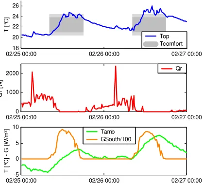
Figure 2: Typical sunny mid-season days, conventional controller

A first attempt was made to tune a detailed TRNSYS (Klein et al., 2000) model of the building. However, the very large number of parameters in the building model makes parameter identification a complex problem. The desired level of accuracy is also quite high, since performance differences of less than 10% must be reproduced.

A simplified model similar to the internal model of the controller was used (linear state-space model). It allows easier identification of some varying parameters (e.g. infiltration rate) and other poorly known influences (e.g. unmeasured heat gains). While such a model is not as well adapted to design studies as a detailed model such as TRNSYS Type 56, it was found to offer more flexibility in parameter identification. The building model is combined with a model of the occupant's reaction to the comfort conditions to account for window opening, as described here above.

Table 4 and Table 5 illustrate results obtained when comparing the conventional controller and the optimal controller on two 1-month periods presenting different meteorological characteristics and using the identified model to extrapolate the performance comparison. The first part of each table sums up the meteorological parameters of the considered period. Comfort and energy parameters are given:

• as measured on the real building (with conventional controller for period 1, with optimal controller for period 2)

• as simulated for the controller that was actually used (model validation)

• as simulated for the other controller

Table 4: Weather data statistics, measured and simulated controller performance – Period 1

Variable Conv, (Meas.)

Conv (Simul.)

Opt (Simul.)

Tamb,min [°C] -1.4

Tamb,max [°C] 18.7

Tamb,avg [°C] 7.0

HSavg [MJ m-2] 9.6

Je [MJ] 470 486 402

Jd,max [%PPD'] 13 10.2 5.4

Jd [%PPD' h] 280 263 215

Table 5: Weather data statistics, measured and simulated controller performance – Period 2

Variable Opt, (Meas.)

Opt (Simul.)

Conv (Simul.)

Tamb,min [°C] -7.3

Tamb,max [°C] 17.2

Tamb,avg [°C] 4.6

HSavg [MJ m-2] 4.4

Je [MJ] 686 708 760

Jd,max [%PPD'] 6.7 4.9 3.0

Jd [%PPD' h] 200 194 190

The results show a very good agreement between simulation and experiments: the energy performance is reproduced within 3.5%. The larger error on the discomfort cost (6% on total, 27% maximum during 0.25 h) is due to the non-linear shape of the cost function (Based on Fanger's PPD), which amplifies the error on operative temperature.

The comparison shows that energy savings of 20% can be achieved during the first period (sunny mid season) while improving the thermal comfort by 18%. During the cold period 2, energy savings of 7% can be achieved with a maintained thermal comfort (small increase of discomfort: 2%).

RESULTS ON THE PASSYS TEST CELL

Controllers

The reference controller (Ref) is an ON/OFF differential controller with hysteresis. It compares the zone temperature (Tz) with a setpoint (Tz,set) and starts

or stops the electrical heater according to the comparison of these two temperatures with two dead band temperatures (∆TLow and ∆THigh) and the

previous state of the control signal. The controller also implements some rules of thumb to prevent unnecessary heating at night (a larger tolerance is allowed on the setpoint). ∆TLow and ∆THigh are

respectively equal to -0.5 and 0.7. This controller uses a fixed schedule to start the heating some time steps prior to (fictitious) occupancy start.

The optimal controller (Opt) is described in (Kummert, 2001). It is based on a simplified state-space model of the test cell and realizes a forecasting of the weather data with a 12-h horizon. The optimization process simulates possible control sequences for the next 12 hours, and finds the optimal one according to a performance criterion which is a linear-quadratic approximation of (3). The value of the α parameter was selected in order to obtain results that were comparable to those of the reference controller.

Available data sets

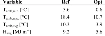
Two 2-week periods of usable data were recorded during this short-term test. The weather data statistics are given in Table 6. Here again, significant differences between the two periods make a direct comparison impossible. The optimal controller was tested in much colder and cloudier conditions.

Table 6: Weather data statistics for the data sets

Variable Ref Opt

Tamb,min [°C] 3.6 0.6

Tamb,max [°C] 18.4 10.7

Tamb,avg [°C] 10.3 3.9

Havg [MJ m-2] 9.2 5.6

Performance comparison using simulation

Here again, a simplified linear state-space model was selected. It uses the structure of the optimal controller's internal model and allows efficient parameter identification.

The parameters of this simplified model were identified using the whole data set (periods 1 and 2). Constant values were identified for all parameters except for air infiltration and solar transmittance. The configuration of the test cell during this study was found to be very sensitive to the wind speed, so the

infiltration was allowed to vary between 1 and 10 vol/h. The global solar transmittance (i.e. the ratio of solar radiation entering the test cell to total incident solar radiation) was allowed to vary in a range from 0.12 to 0.6 to take into account the variation of glass transmittance with incidence angle and the effect of un-modeled shading. This attenuation factor corresponds to a transmittance ranging from 0.1 to 0.5 for a 1.2 m² glazed area.

Figure 3 shows the zone temperature during both periods, for simulation-based and experimental results. The low thermal capacitance of the building and the ON/OFF nature of the heating system lead to instantaneous discrepancies, but the behaviour of the entire system (building + controller) is very well reproduced by the simulation.

11/30 12/01 12/02 12/03 12/04 12/05

16 18 20 22 24 26

T [

°C

]

Tin Meas Tin Sim

01/11 01/13 01/15

14 16 18 20 22 24

T [

°C

]

Figure 3: simulated and measured air temperature, PASSYS test cell

Table 7 and Table 8 illustrate the results obtained when comparing the reference controller and the optimal controller on the two 2-week periods. Comfort and energy parameters are given:

• as measured on the real building (with conventional controller for period 1, with optimal controller for period 2)

• as simulated for the controller that was actually used (model validation)

• as simulated for the other controller

Table 7:Measured and simulated controller performance – Period 1

Variable Ref, (Meas.)

Ref (Simul.)

Opt (Simul.)

Je [MJ] 94 92 70

Jd,max [%PPD'] 11.2 11.2 5.8

Jd [%PPD' h] 0.9 0.7 0.36

PMVmin -0.10 -0.11 -0.42

PMVmax 0.76 0.77 0.54

PMVavg 0.10 0.08 0.02

Period 1, Ref controller

Table 8: Measured and simulated controller performance – Period 2

Variable Opt, (Meas.)

Opt (Simul.)

Ref (Simul.)

Je [MJ] 295 296 314

Jd,max [%PPD'] 2.6 3.8 0.89

Jd [%PPD' h] 0.20 0.23 0.03

PMVmin -0.36 -0.43 -0.21

PMVmax 0 0 0

PMVavg -0.05 -0.06 -0.02

The results show a very good agreement between simulation and experiments for the controllers that were actually implemented in the test cell. The energy consumption is reproduced within 2.6% in the worst case. The more important error for discomfort cost is mostly due to the non-linear shape of Jd: very

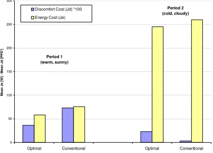
small errors on maximum or minimum temperatures during the day have a large effect on the discomfort cost. However, the agreement is still very good. A more visual rendering of the comparison between different controllers for the same period (columns 3and 4 of Tables 7 and 8) is presented in Figure 4.

0 50 100 150 200 250 300

Optimal Conventional Optimal Conventional

Mean Je [

W

]

Mean Jd [

PPD'

]

Discomfort Cost (Jd) *100 Energy Cost (Je)

Period 1 (warm, sunny)

Period 2 (cold, cloudy)

Figure 4: performance comparison based on simulation results, PASSYS test cell

When comparing the performance of both controllers for the same period, The comparison shows that important energy savings (25%) can be achieved with an improved comfort during period 1 (warm and sunny). Even if the implemented reference controller was not optimized for these conditions (it used a rather conservative fixed schedule), this confirms that most of the savings and comfort improvement can be achieved during mid-season.

For the cold period, the optimal controller with implemented settings (mid-range comfort level) gives 6% energy savings, but at the cost of a higher discomfort. A look at Figure 3 (lower part) allows understanding why the discomfort cost is so high. On the second day, the temperature goes down to 19°C during the occupation period. However, the setpoint

was reached before the start of the occupancy, so the problem is not caused by a poor anticipation of the building's behavior. The cause is that the ON/OFF control of heating is not well handled by the optimal controller, which was developed for hydronic systems.

CONCLUSIONS

The methodology of performance comparison by combining simulation and experiments has been applied successfully to an occupied passive solar building and to the PASSYS test cell.

The experiments on the test cell were very valuable to the study, in spite of their short time span. First, they allowed to assess the performance of the developed optimal control algorithm in a very different context: ON/OFF control, very low thermal mass building. Secondly, the well-controlled environment offered an ideal test case to test the modeling and parameter identification methodology. That methodology was then adapted to the real building, where the influence of adjacent rooms and occupants had to be added.

Adding simulation results to the experimental comparison allows to estimate yearly savings and to study the behavior of controllers with different weather or occupancy conditions, therefore adding useful information to the comparison.

Considerable care must be taken when defining the structure of the building model (e.g. include a model of the occupants reaction rather than its effects) and identifying the parameters, to avoid the risk of over-fitting. At the same time, the simulation should be able to reproduce performance differences that are in the range of 10%, which requires a very good accuracy. It is interesting to note that the ever-increasing computational power has made possible to consider using detailed, physically-based, models for inclusion in the control algorithm itself (Clarke et al., 2001). This study, however, has shown that parameter identification is a crucial point both for the controller's internal model and for models used in assessing the controller's performance. Detailed building models require thousands of parameters, which makes them unsuitable for classical parameter identification techniques.

ACKNOWLEDGMENTS

This work has been partly funded by the European Commission, Directorate General XII (Contract JOE3-CT97-0076). The authors also thank the Belgian national weather institute (Institut Royal Météorologique) for providing the email-based weather forecasts used by the optimal controller.

NOMENCLATURE

Variable Units Description

ATavg [°C] Average Daily amplitude of the

temperature

Havg

Hmin

Hmax

[MJ m-2_{] Daily horizontal solar radiation}

(average, minimum and maximum)

HSavg

HSmin

HSmax

[MJ m-2_{] Daily solar radiation on the South}

façade (average, minimum and maximum)

Jd [PPD' h] Discomfort "cost" (see text)

Jd,avg [%PPD'] Discomfort "cost", average Jd,max [%PPD'] Discomfort "cost", maximum

Je [MJ] Energy "cost" (see text)

PMVmin [-] Predicted Mean Vote, minimum

PMVmax [-] Predicted Mean Vote, maximum

PMVavg [-] Predicted Mean Vote, average

PPD [%] Predicted percentage of

Dissatisfied people

Tamb [°C] Ambient temperature

Tamb,avg Tamb,min Tamb,max

[°C] Average, minimum and maximum

ambient temperature

Top [°C] Operative temperature (ref. zone)

Tcomfort [°C] (Approximative) Comfort zone GSouth [W m-2] Radiation on South façade

Tws [°C] water supply temperature

Twr [°C] water return temperature

REFERENCES

Clarke J.A., Cockroft J., Conner S., Hand J.W., Kelly N.J., Morre R., O'Brien T. and Strachan P, 2001. Control in building energy management systems: the role of simulation. In Proceedings of the 7th International Building Performance Simulation Association (IBPSA) Conference 2001, Rio de Janeiro, Brazil.

Fanger P.O., 1972. Thermal comfort analysis and application in environmental design. Mac Graw Hill.

Flake B.A., 1998. Parameter estimation and optimal supervisory control of chilled water plants. Ph. D. Thesis. University of Wisconsin-Madison

Keeney K. and Braun J.E., 1996. A simplified method for determining optimal cooling control strategies for thermal storage in building mass. HVAC&R Research, Vol. 2, Nb. 1

Kolokotsa D., 2003. Comparison of the performance of fuzzy controllers for the management of the indoor environment. Building and Environment, Environment, 38 pp. 1439 – 1450

Kummert M., 2001. Contribution to the application of modern control techniques to solar buildings. Simulation-based approach and experimental validation. Ph. D. Thesis, Fondation Universitaire Luxembourgeoise (Now University of Liège, Department of Environmental Sciences and Management), Arlon.

Kummert M., André Ph., 2005. Simulation of a model-based optimal controller for heating systems under realistic hypotheses. IBPSA Building Simulation 2005 conference, Montréal, Canada.

Mozer, M.C., Vidmar, L., Dodier, R.H., 1997. The neurothermostat: predictive optimal control of residential heating systems. In Proceedings of Advances in Neural Information Processing Systems 9, MIT Press, Cambridge, MA, pp. 953-959.

Nygard-Fergusson A.-M., 1990. Predictive thermal control of building systems. Ph. D. Thesis. Ecole Polytechnique Fédérale de Lausanne

Oestreicher Y., Bauer M. and Scartezzini J.-L., 1996. Accounting free gains in a non residential building by means of an optimal stochastic controller, Energy and Buildings, 24, pp. 213-221.

Van Dijk H.A.L. (editor), 1994. The PASSYS project. Development of the PASSYS test method. Research report of the subgroup test methodologies. European Commission, D.G. XII, Brussels.

Van Schijndel A.W.M., 2002. Optimal operation of a hospital power plant. Energy and Buildings, 34, pp.1055-1065.