Einstein-Gauss-Bonnet gravity with extra dimensions

White Rose Research Online URL for this paper:

http://eprints.whiterose.ac.uk/144164/

Version: Published Version

Article:

Bruck, C.V.D. and Longden, C. (2019) Einstein-Gauss-Bonnet gravity with extra

dimensions. Galaxies, 7 (1). 39. ISSN 2075-4434

https://doi.org/10.3390/galaxies7010039

[email protected] https://eprints.whiterose.ac.uk/ Reuse

This article is distributed under the terms of the Creative Commons Attribution (CC BY) licence. This licence allows you to distribute, remix, tweak, and build upon the work, even commercially, as long as you credit the authors for the original work. More information and the full terms of the licence here:

https://creativecommons.org/licenses/

Takedown

If you consider content in White Rose Research Online to be in breach of UK law, please notify us by

Article

Einstein-Gauss-Bonnet Gravity with

Extra Dimensions

Carsten van de Bruck * and Chris Longden

Consortium for Fundamental Physics, School of Mathematics and Statistics, University of Sheffield, Hounsfield Road, Sheffield S3 7RH, UK; [email protected]

*Correspondence: [email protected]

Received: 28 January 2019; Accepted: 12 March 2019; Published: 19 March 2019

Abstract: We consider a theory of modified gravity possessingd extra spatial dimensions with a maximally symmetric metric and a scale factor, whose(4+d)-dimensional gravitational action contains terms proportional to quadratic curvature scalars. Constructing the 4D effective field theory by dimensional reduction, we find that a special case of our action where the additional terms appear in the well-known Gauss-Bonnet combination is of special interest as it uniquely produces a Horndeski scalar-tensor theory in the 4D effective action. We further consider the possibility of achieving stabilised extra dimensions in this scenario, as a function of the number and curvature of extra dimensions, as well as the strength of the Gauss-Bonnet coupling. Further questions that remain to be answered such as the influence of matter-coupling are briefly discussed.

Keywords:cosmology; extra dimensions; early universe

1. Introduction

There is no concrete a priori reason the spacetime we live in should have precisely three spatial dimensions and one time dimension (for overviews of diverse theories with extra dimensions and their physical consequences see e.g., [1–4]. Instead, theoretical physicists hope that a fundamental theory of nature will be able to predict the number of dimensions of spacetime. In string theory, for example, consistency requires additional spatial dimensions. At the very least, a theory proposing more than three spatial dimensions requires the additional dimensions to be either small in order to be physically plausible or require objects like branes, on which standard model particles are confined, in order for the theory to be consistent with observations. A central question in such theories is, then, how these extra dimensions become sufficiently small and/or stabilise, given the field content and dynamics of such theories.

It has been established for a long time that extra-dimensional theories can, in the appropriate limit, behave like a conventional four-dimensional spacetime with additional field content derived from the influence of the extra dimensions. Kaluza-Klein theory, in which one obtains gravity and electromagnetism in four dimensions by starting from gravity alone in five dimensions, is the textbook example. More modern realisations of this paradigm, including the work to be presented in what follows, often parametrise the size of the extra dimensions with a scalar field, leading to an effective 4D action which is a scalar-tensor theory. Similarly, one can consider, particularly in string theory contexts, the influence of D-branes and other objects found in the extra-dimensional space on our perceived four-dimensional world to produce scalar-tensor and vector-tensor theories with interesting properties.

Extra dimensions, as well as being of general interest in theoretical physics, have particular applications and consequences in the context of cosmology. Questions on the nature of dark matter and dark energy could potentially have resolutions in theories of matter existing in hidden extra dimensions, or of extra-dimensional effects on the dynamics of the observed four-dimensional universe. Similarly,

early-universe phenomena such as inflation could be driven by extra-dimensional effects, or at least occur in the presence of extra-dimensions. For work in these directions, see [5–13].

For many purposes of interest, it is useful if extra dimensions can be stabilised in size to a high precision. Not only does this come with the desirable property of avoiding problems associated with an endless collapse down to the uncharted territory of poorly understood Planck-scale effects or the evolution of fundamental constants, but it also lends itself well to, say, application to dark energy. Cosmological observations indicate that that the energy density of dark energy is either very close to, or exactly, constant, and in scalar-tensor theories, this is often due to a frozen, non-evolving, scalar field. When thinking about extra dimensions, this is most immediately understood, then, as a constant-size extra-dimensional space. A constant or near-constant energy density is also desirable from the perspective of inflation.

As the introduction of additional spatial dimensions often modifies gravity in the four-dimensional effective action, there will unavoidably be questions regarding the compatibility of such theories with local constraints on deviations from General Relativity (GR). This is another problem that may be alleviated if the extra dimensions are sufficiently stabilised that they do little more than contribute vacuum energy at present, while keeping open the possibility that larger and more dynamic extra-dimensional effects were present in the early universe where constraints are weaker.

Unfortunately, it is not a trivial task to stabilise extra dimensions. If gravity in the full extra-dimensional theory is described by GR one typically does not find such situations in which one (or several) dimensions are stabilised. In fact, it has been argued that it is highly non-trivial in GR to stabilise extra dimensions [14]. Instead, within GR, all dimensions want to be dynamical (for a disucssion on Kaluza-Klein gravity and its consequences, see [2]). This motivates our work in this paper in which we study an extended theory of gravity. In particular, we add terms proportional to all quadratic curvature scalars to the action. From an effective field theory perspective, it is these terms that we would expect to bring leading order corrections to GR, and they are indeed often generated in high energy theories (for a discussion see e.g., [15]). Starobinsky’sR2_{gravity is the most well-known} example. It is the hope that these contributions generate an effective potential for the scale factor of the extra dimensions, which in the low-energy effective field theory is a scalar field.

electromagnetic counterpart of the binary neutron star merger GW170817 [25] implies that gravitational waves propagate with the speed of light. A GB correction which is important at late times would not be compatible with this results and therefore the extra-dimensions have to be frozen at late times in a set-up described in this paper [26–29]. Thus, we believe that if the GB term has any relevance for stabilising the extra dimensions, it has to do so in the very early universe, possibly during inflation. In addition, we would like to establish the link of the higher-dimensional theory to the Horndeski theory in 4D.

The paper is organised as follows. In the next Section, we describe the general setup in

(4+d)dimensions and determine the four-dimensional effective action. As we will see, in the case of a(4+d)-dimensional Einstein-Gauss-Bonnet theory, the effective four-dimensional theory is of Horndeski form, in which the scale factor describing the size of the extra dimensional submanifold is a scalar field. In Section3we discuss some properties of the resulting 4D theory. In particular we look for minima in the effective potential. We also briefly comment on the inclusion of matter. Our conclusions can be found in Section4.

2. A Theory of Modified Gravity with Extra Dimensions

We first consider a theory of gravity constructed in(4+d)spacetime dimensions in which the usual(4+d)-dimensional Ricci scalar,R, is accompanied by an arbitrary cosmological constant and terms proportional to the three quadratic-order curvature scalarsR2,RµνRµνandRρσµνRρσµν, that is,

S= M

2+d

4+d

2

Z

d(4+d)X√₋GR+c1R2+c2RABRAB+c3RABCDRABCD−2Λ4+d

, (1)

where capital Roman indices run from 0 . . .d +3 and denote objects defined on the full

(4+d)-dimensional manifold. The metric in(4+d)dimensions,G, is to be understood as a product metric built from a 4-dimensional metricgand ad-dimensional metricγsuch that

ds2=GABdXAdXB=gαβ(x)dxαdxβ+b(x)2γmn(y)dymdyn, (2)

where we use Greek letters and lower case Roman letters to label objects defined on the 4-dimensional (4D) andd-dimensional components respectively. As such, our ansatz for the(4+d)-dimensional spacetime is similar to the one used in [23]. Similarlyxα_{is used to represent the coordinates on the} 4-dimensional spacetime andymthose of thedextra dimensions. In the above we have introduced a scale factor b(x)controlling the size of the d extra dimensions which is only a function of the 4-dimensional coordinates. For simplicity, we make the assumption thatγis the metric of a maximally symmetric space with Ricci curvatureRd.

To study the 4D effective action of the above theory, we will perform dimensional reduction. The steps are very similar to the one presented in [14]. In this process, one decomposes the theory into tensor and scalar parts, where the scalar field is identified with thed-dimensional metric’s scale factor,b. As this only depends onxα_{(and because of our previous assumption of maximal symmetry} inγ), the part of the action depending on coordinatesya can be factored out of the action integral such that

S= M

2+d

4+d

2

Z

d4xddyp

−g√γbdL4D =

M2+₄₊d_dV

2

Z

d4xp

−gbdL4D, (3)

where

V=

Z

ddy√γ, (4)

well as the scale factorb. After straightforward but tedious computations, one finds it can be written in the form

L4D =L4+Ld+Lb−2Λ4+d, (5)

whereL4is a four-dimensional gravity sector containing a non-minimal (kinetic) coupling between

band the 4D Ricci scalarR4, the same quadratic curvature terms as the original higher-dimensional action, as well as a coupling of the 4D Ricci Tensor to the derivatives of the field

L4 = "

1+2c1 R_b2d − d(d−1)

b2 (∇b)2 − 2bd(b)

!#

R4

+c1R24+c2RαβRαβ+c3RαβγδRαβγδ − 2dcb2Rαβ∇α∇βb.

(6)

Similarly, Ld contains terms that look like non-minimal gravity for thed-dimensional part of the metric

Ld =

"

1 − 2d(d−1)c1+(d−1)c2+2c3

b2 (∇b)2 − 2

2dc₁+c2 b (b)

#

Rd b2

+ hc1+cd2 +

2c3 d(d−1)

i_R2 d b4 ,

(7)

where in the last term maximal symmetry has been used to express the squares of the Ricci and Riemann tensors in terms of the constant Ricci scalarRd.1Because of this, while it resembles gravity inddimensions, it is better identified as kinetic and potential terms for the scalar degree of freedom that are proportional to the extra-dimensional curvature (and its square).

Additionally, we find terms corresponding to a Lagrangian for thebfield that does not depend on

Rd, contributing further kinetic structure to the 4D theory,Lb. This is further comprised of terms with two derivatives, terms with four derivatives acting on different combinations of 2, 3 and 4 factors of b.

Lb=−d 2

b(b) + d−1

b2 (∇b) 2

!

+Lb2+Lb3+Lb4, (8)

where the two-factor term is

Lb2=

d(dc2+4c3)

b2 (∇α∇

β_b)(∇α_∇ βb) +

d(4dc1+c2)

b2 (b)

2 _{, (9)}

the three-factor term is

Lb3=

2d(d−1)(2dc1+c2)

b3 (∇b)

2₍

b), (10)

and finally the four-factor term is

Lb4=d(d−1)

d(d−1)c1+ (d−1)c2+2c3

b4 (∇b)

4_{. (11)}

2.1. Gauss-Bonnet and Horndeski Theory

A special case of our action in Equation (1) is whenc1 = c3 = −c2/4 = −ξ, leading to the ubiquitous Gauss-Bonnet combination of quadratic curvature scalars. While in four dimensions it is a total derivative, in higher dimensions or when non-minimally coupled it plays a role in gravity. Using our results above from Equations (6)–(11) with this choice of coupling constants, the full 4D action (3) can be written in the form

1 _{This expression is invalid in the cased=1. The physical reason for this is that a one-dimensional space has identically zero}

S= M

2+d

4+dV

2

Z

d4xp

−ghLH−ξbdR2GB i

, (12)

whereR2

GB=R2−4RµνRµν+RρµσνRρµσνis the 4D Gauss-Bonnet term,2which, as it is non-minimally coupled via a factor ofbdcoming from the reduction of the metric determinant in the integration measure, is non-negligible. The other term present isLH, a Horndeski theory Lagrangian

LH=G4(b,X)R4+P(b,X)−G3(b,X) (b) +G4,X

h

(b)2−(∇α∇βb)(∇α∇βb)

i

+G5(b,X)Gαβ∇α∇βb−

1 6G5,X

h

(b)3−3(b) (∇α∇βb)(∇β∇αb) +2(∇α∇βb)(∇β∇γb)(∇γ∇αb)

i

, (13)

where

P(b,X) =K(b,X)−V(b) (14)

K(b,X) =

2d(d−1)−4ξRd(d_b2−2)

bd−2X−4ξd(d−1)(d−2)(d−3)bd−4X2, (15)

V(b) =2Λ_4+dbd_−Rdbd−2_+ξ(d−2)(d−3)

d(d−1) R

2

dbd−4, (16)

G3(b,X) =2dbd−1−4ξRd(d−2)bd−3−8ξd(d−1)(d−2)bd−3X, (17)

G4(b,X) =1−2ξRdbd−2−4ξd(d−1)bd−2X, (18)

G5(b) =−8dξbd−1. (19)

where the kinetic term for the scalar field b is denoted with the common convention of

X=−∇µ_b∇

µb/2. Note the(4+d)-dimensional cosmological constantΛ4+dis absorbed into this

action as the prefactor for thebdterm (again resulting from the metric determinant) in the scalar potentialV(b).

It is well known that the coupled Gauss-Bonnet term in four dimensions is in itself also a Horndeski theory [30]. Using the equations in Appendix B3 in [30], we can transform the Gauss-Bonnet term accordingly. The action (12) is, therefore, the sum of two Horndeski theories, and thus, a Horndeski theory itself. In fact, by explicitly rewriting the Gauss-Bonnet sector in Horndeski-like form, one can obtain the action in “pure Horndeski” form

S= M

2+d

4+dV

2

Z

d4xp

−gLH, (20)

where now the DGSZ potentialsKandGnobtain logarithmic corrections inX, taking the modified form,

P(b,X) =K(b,X)−V(b) (21)

K(b,X) =

2d(d−1)−4ξRd(d_b2−2)

bd−2X−4ξd(d−1)(d−2)(d−3)bd−4_X2_{(7−2 ln|X|), (22)}

V(b) =2Λ_4+dbd_−Rdbd−2_+ξ(d−2)(d−3)

d(d−1) R

2

dbd−4, (23)

G3(b,X) =2dbd−1−4ξRd(d−2)bd−3−12d(d−1)(d−2)ξbd−3X(3−ln|X|), (24)

G4(b,X) =1−2ξRdbd−2−4d(d−1)ξbd−2X(3−ln|X|), (25)

G5(b,X) =−4dξbd−1(2−ln|X|). (26)

2 _{For notational simplicity, we will henceforth omit the subscript inR}

4when referring to the 4D Ricci Scalar, as the full

We conclude that higher-dimensional Einstein-Gauss-Bonnet gravity, with maximally symmetric extra dimensions and a metric ansatz of the form (2), the four dimensional effective action is simply a Horndeski-class scalar-tensor theories whose particular potentials have been computed and presented above. This is the form of the theory which is typically easiest to work with, given the abundance of literature on Horndeski theories as a standardised template of many scalar-tensor theories. It also confirms without explicit calculation that the theory has stable second-order equations of motion. We should emphasise that the logarithmic terms in the DGSZ potentials do not lead to pathologies in the equations of motion: these terms are usually multiplied byXand therefore finite in the limit when

X→0. A similar situation appears in the theory presented in [31].

3. Some Properties of the 4D Effective Theory

3.1. Specialness of the Gauss-Bonnet Case

The results of Section2.1show that choosingc1=c3=−c2/4=−ξor any constant multiple of this leads to a 4D effective action in the form of a Horndeski theory. It turns out this is a special result in that other choices of thecn coefficients do not lead to Horndeski theories. For example, consider the four-derivative terms in Equation (9). Typically, terms with four derivatives do not correspond to second order equations of motion, but Horndeski’s theory tells us that specific combinations of such higher derivative interactions can cancel out each others’ pathological elements, leading to an overall stable theory. In the Gauss-Bonnet case, the specific terms in question correspond to the following terms in the Horndeski action:

LH⊃G4,X

h

(b)2−(∇α∇βb)(∇α∇βb) i

. (27)

This identification is possible because in Equation (9), the choicec1=c3=−c2/4=−ξmakes the coefficients of(b)2and(∇α∇βb)(∇α∇βb)equal up to a sign difference; in the Horndeski action these two terms must appear in this form in order to cancel out parts that do not lead to second order contributions to the equations of motion. We see that general choices ofcndo not generally lead to Horndeski-compatible theories in 4D. In fact, upon a more comprehensive study of the correspondence between the 4D effective action and Horndeski-allowed terms, one can prove that the Gauss-Bonnet combination is the only choice ofc1,c2andc3that will lead to a Horndeski theory. We present the proof of this uniqueness in AppendixA.

It is interesting that the Gauss-Bonnet term’s specialness among combinations of quadratic curvature scalars manifests in this way. Please note that this means that even the higher-dimensional analogue of the well-studied Starobinsky orR2theory of modified gravity

S= M

2+d

4+d

2

Z

d(4+d)X√−GR+αR2−2Λ_{4+d, (28)}

would reduce in 4D to a theory that is not Horndeski. As well as the fact that the structure of the

bfield’s Lagrangian would have greater than second order equations of motion, a residualR2term would persist in the 4D action, and could in principle be conformally transformed into a second scalar field that interacts non-trivially withb. It is not immediately clear that this interaction would avoid pathology in b’s dynamics, but as the full(4+d)-dimensional theory should be stable, one might hypothesise that its dimensionally reduced form is no different, though testing this explicitly is beyond the scope of the present work. Given the speciality of the Gauss-Bonnet combination, its physical relevance, and the relative simplicity of its 4D effective action compared to Starobinsky theory or another choice ofcn, we will henceforth focus on the special case of the action (1) given by

S= M

2+d

4+d

2

Z

3.2. Effective 4D Planck Mass and Cosmological Constant

We will discuss below the properties of effective potential for the fieldband whetherbcan in principle stabilise at all. Assuming for now that a static solutionb=b0is reached and this persists until late-time cosmology, we can evaluate the effective cosmological constant and four dimensional effective Planck mass resulting from this. Directly broadcasting the 4D effective action (12) into a form where the prefactor of the Ricci Scalar isM2₄(b,X)/2 gives us the equation

M₄2(b,X) =G4(b,X)M₄₊2+d_dV ≡G4(b,X)α. (30) Here we have introduced the notationα=M₄₊2+d_dVbecause as we have seen already in Section2, this combination appears very often in the four–dimensional effective theory. Explicitly using the form ofG4given in Equations (21)–(26), and evaluating at the point (b=b0,X=0) we find that the observed (constant) Planck-mass today would be

M2₄= (1−2ξRdbd0−2)α. (31)

Enforcing that this equality holds for the measured value ofM4, coming from say a weak-gravity experimental determination of Newton’s constant, constrains one parameter of the theory. It is helpful to rewrite the 4D effective action using this expression forM2₄such that theG4coupling takes the form

G4(b,X) =1−2ξRdbd−2−4d(d−1)ξbd−2X(3−ln|X|), =1−2ξRdb0d−2−2ξRd

bd−2−b₀d−2−4d(d−1)ξbd−2X(3−ln|X|),

= M

2 4

α −2ξRd

bd−2−bd₀−2−4d(d−1)ξbd−2X(3−ln|X|), (32)

where in the first step we have added and subtracted(2ξRdb0d−2), and in the second step we have used the definition ofM2

4. The action now can be written in a form explicitly containing the 4D Planck Mass such as

S= M

2 4 2

Z

d4xp

−gR + α

2

Z

d4xp

−gL¯H, (33)

where ¯LHis the same Horndeski Lagrangian specified by Equations (21)–(26), exceptG4is replaced with ¯G4, defined by

¯

G4(b,X) =G4(b,X)−G4(b0, 0), (34)

=G4(b,X)−

M2₄

α , (35)

=−2ξRd

bd−2₋b₀d−2₋4d(d−1)ξbd−2X(3₋ln_|X_|), (36)

where in the second line we have used (32).

Similarly, one can show that the 4D effective cosmological constant for a stabilised field is simply

Λ₌ α

2M2₄V(b0) =

α

2M2₄

2Λ_4+db4_0−Rdb02_+ξR2_d(d−2)(d−3)

d(d−1)

bd₀−4, (37)

and this would allow us to write the action in a form

S= M

2 4 2

Z

d4xp

−g(R−2Λ_{) +} α 2

Z

d4xp

where now the barred Horndeski Lagrangian ¯LHis again specified by Equations (21)–(26), this time with bothG4andVreplaced by barred variations given respectively by (34) and

¯

V(b) =V(b)−V(b0). (39)

The action (37) then has the property that the second term containing the Horndeski Lagrangian vanishes whenb=b0, as all the parts not proportional to derivatives ofb(i.e.,X) have been absorbed into the definitions of the effective Planck mass and cosmological constant in the first term, and

¯

G4(b0) =V(b¯ 0) =0 by construction.

3.3. Effective Potential and Static Solutions

We will now address the question under which circumstances the effective potential has at least one minimum. This is a necessary condition for the extra dimension, whose dynamics is described by the scalar–fieldb, to stabilise. Please note that this condition itself is not sufficient: the dynamics of the fieldbhas to be such that it is driven towards the minima of the effective potential. We will study this in future work, in particular in the context of inflation and whetherbitself can be an inflaton field.

In the limit of negligible motion of the field, the Friedmann and Klein-Gordon equations (whose full forms can be found e.g., in [32]) can be approximated at zeroth order in ˙b, and take the form

6H2G4=V (40)

V,b+12H2G4,b =0 . (41)

Using the equations of motion in this form allows us to search for static solutions of the system—those in which the field is frozen in place. These are of particular interest in the context of cases such as ours where the field represents the size of extra dimensions, as it implies their stabilisation, as well as the context of cosmology where static scalar fields in a potential behave as fluids with equation of state of−1. Particularly when thinking about stabilisation of the extra dimensions, we are also interested in static solutions whereb=b06=0 as this would imply extra dimensions of zero size, which has obvious difficulties in interpretation.

The presence of terms other thanV,bin the Klein-Gordon equation implies that even in the static

limit, the points at which the field can sustain a constant value will not be the minima of the bare potential V but instead some effective potential due to a combination ofV and G4. As we have neglected motion of the field in this, this calculation also makes no claims regarding whether the system can dynamically reach such a stable point3, simply whether stable points exist. What we can say from such an analysis is whether such static solutions exist in the first place, and if so what the sufficient, necessary or preferable conditions for their existence are in terms of say the number of dimensions and the combination of model parameters such asξandRd4. In this limit of negligible field motion, the static solutions we find will also be stable to zeroth order in ˙bas long as they occur at minima of the effective potential (e.g., in the slice ˙b=0. Their stability against small perturbations in the field velocity, however, is also dependent on the matter coupling, and cannot be fully addressed within the scope of the present work.

In conventional scalar-tensor theory, the equation of motion is justV,b =0, and so it is natural to

define an effective potential gradientVeff,b =V,b+12H2G4,bto mimic this form. Using the Friedmann

3 _{In Section3.4we will argue that one should include the effects of matter in any such discussion of dynamics, and that the}

arbitrariness of how matter is coupled means that a more comprehensive future study of this needs to be done to fully understand such questions.

4 _{Narrowing down the parameter space now to only those models in which an interesting static solution exists will be an}

equation to eliminateH2from this expression and using the specific forms ofVandG4for our theory gives the effective potential gradient as

Veff,b=V,b+2 G4,b

G4

V,

=2dΛ_4+dbd−1_{−(d−2)Rdb}d−3₊ (d−2)(d−3)(d−4)

d(d−1) ξR

2

dbd−5

− 4(d−2)ξRd

1−2ξRdbd−2

2Λ_4+db2d−3_−Rdb2d−5₊(d−2)(d−3)

d(d−1) ξR

2

db2d−7

(42)

= 1

1−2ξRdbd−2

"

2dΛ_4+dbd−1_{−(d−2)Rdb}d−3₊(d−2)(d−3)(d−4)

d(d−1) ξR

2

dbd−5

−4(3d−4)Λ_4+dξRdb2d−3_+6(d−2)ξR2

db2d−5−2

(d−2)(d−3)(3d−8)

d(d−1) ξ

2_R3

db2d−7

#

. (43)

Finding solutions toVeff,b = 0 to identify the existence of static solutions, using the effective

potential as given by (43), then reduces to a problem of solving a polynomial equation of six terms with orders(d−1),(d−3),(d−5),(2d₋3),(2d₋5), and(2d₋7). This is, of course, not generally possible for either generaldnor for any specified value ofd. Below we will look at each choice ofdas a special case and categorise the possible behaviours.

Before proceeding to this, however, we can also directly integrate the expression (42) or (43) with respect tobto see what the effective potentialVeffitself looks like, i.e., what corrections do the presence of aG4term impose on the shape of the potential felt by the field in the limit of negligible motion. This procedure yields the expression,

Veff=2Λd+4bd−3Rdbd−2+ξ

(d−2)(d−3) d(d−1) R

2

dbd−4−

1

ξlog

1₋2ξRdbd−2

−2ξ2R3_d

(d−2)2

d(d−1)

×2F1

1,2(d−3)

d−2 ; 3d−8

d−2 ; 2ξRdb

d₋2_b2(d₋3)

−4ξRdΛ_d+4

d−2

d−1

×2F1

1,2(d−1)

d−2 ; 3d−4

d−2 ; 2ξRdb

d₋2_b2(d₋1)_{, (44)}

where2F1is the hypergeometric function. Note the structure of this potential: the first three terms are as in the bare potential, with the difference that the coefficient of the second term is now 3 instead of 1. Furthermore, logarithmic and hypergeometric correction terms are generated. The logarithmic term in particular imposes a boundary on the valuesbmay take if the reality of the potential is enforced, that is

2ξRdbd−2<1 . (45)

This is trivially satisfied if the sign of the combination of terms on the left hand side is negative, but when it is positive there will generally be some limit on the value ofb. As well as representing a divergence in the effective potential, this inequality also imposes essentially the positivity ofG4and that ofH2in the Friedman equation (assumingVis also positive) as well as that of the effective square Planck mass, a topic that will be more explicitly discussed in Section3.2.

parameters must be to actually replicate the observed cosmological constant as our foremost interest here is to exclude models and numbers of dimensions on grounds of wider criteria rather than precise and comprehensive parameter searches.

3.3.1. Case ofd= 1 or 2

In d = 1 the expressions derived in this work are largely simplified by the fact that a one-dimensional space has zero Ricci curvature. One result of this is that the effective potential is just the bare potential, which in the limit ofRd=0 is simplyV=2Λ5b. Similarly, the expression for the effective potential in Equation (44) is invalid for the cased= 2, as in this caseG4,b = 0 and

therefore the effective potential is identical to the bare potential, which takes the formV=2Λ_6b2_−Rd. Neither of these cases of are of interest to us, as thed=1 case has a linear effective potential which cannot stabilise, and thed=2 case has a quadratic potential which is capable of stabilising but only at

b=0. We therefore rule out these models. Please note that our findings do not contradict [6], as our starting point with a simple cosmological constant in the bulk is different from the starting point in that paper.

3.3.2. Case ofd≥6

Inspecting the expression forVeff,bin Equation (43), we see that ford≥6,b=0 will always be a

solution of the Klein-Gordon equation, implying a turning point of the potential necessarily exists at

b=0. This alone would not be a problem, if not for the fact that in models withd_≥6 one also finds thatVeff(0) =0 and that the effective cosmological constant at the pointb=0 is also zero (as this is set by the bare potential). These two facts combined mean that if there exists a stable potential minimum point other thanb=0, then it is either not a global minimum, or it possesses a negative cosmological constant. This does not strictly rule out the case ofd _≥ 6 for interesting applications; it is entirely possible that we have a metastable state represented by a non-global minimum in effective vacuum energy. However, as this is an additional complication, we are less inclined to explore this possibility in our initial survey of models. When we, in a future work, return to the question of dynamical stabilisation, such metastable points will be undesirable as we would not expect them to be reached from generic initial conditions.

An additional complication with the class ofd≥6 models is that the leading term in theVeff,b

polynomial is of order(2d₋3), that is, even for the cased=6 we would have to deal with a potential with up to nine possible turning points whosebvalues can not in general be analytically determined.

Given these observations, while we do not absolutely rule out models ofd≥6, we initially choose to relegate them as more convoluted and complex than strictly necessary. We will see next that the remaining cases ofdbetween 3 and 5 provide enough feasible behaviour that we need not delve into this possibility at this stage.

3.3.3. Case ofd=3

Ind=3, the integer arguments of the hypergeometic functions in the effective potential allow us to write it in the simplified form

2

αV

(d=3) eff =−

ξ2R3

d

3 +

Λ₇

ξ2_R2

d

−3Rd

!

b+ Λ7

ξRd

b2+20Λ7

6 b

3₊ Λ7 2ξ3_R3

d

−1_ξ

!

log(1−2ξRdb), (46)

in which the hypergeometric functions can now be seen to simply change the prefactor of the logarithmic correction to the polynomial bare potential. Manipulation of Equation (43) additionally reveals that the turning points of the potential occur atbvalues that are solutions of the cubic equation

b3−₁₀3

ξRd

b2−₁₀3R_Λd

7

b+ 1

As the logarithm in the effective potential imposes 2ξRdb < 1,G4will always be positive for viable field values, and so the sign of the effective cosmological constant is determined entirely by the bare potential, which in this case looks like

Vd=3(b) =2Λ_7b2_{−Rdb. (48)}

As there are an odd number of extra dimensions in this case, it works out that the potential and effective potential take these asymmetrical forms. Considering we wish to interpretbas a scale factor of the extra dimensions, common sense suggests we should imposeb >_{0 to facilitate this.}5

We therefore ignore the possibility of negativeb. Whether the time-evolution of the system, taking matter couplings into account, obeys this is of course left to future work probing the dynamics of our model.

The simplest way to ensure a positive effective cosmological constant is possible, from Equation (48), would be to imposeΛ₇ > _{0 and Rd} < _{0. However, by Descartes’s Rule of Signs,}

we would require in this case thatξ < 0 as a necessary and sufficient condition for a positive-b

turning point to exist. The discriminant of the cubic equation can also be shown to be negative for this combination of signs, identifying this as the sole real root. Then, asRd<_{0, and}

Veff,b(0) =−Rd, (49)

is positive, the single turning point at positive-bwill always be a maximum rather than a minimum, making this case of no use. If we instead chooseRd>0 to ensure that the first turning point at positive b(should it exist at all) be a minimum, thenΛ₇>_{0 is also a necessary but not sufficient condition}

for the positivity ofVat positivebvalues. That is, from (48) we see thatVwill only be positive for

b2 >R_d/Λ_{7. Finally, from arguments again based on Descartes’s Rule, one can only guarantee the} existence of a positive turning point in this situation whenξ < 0, and that there will only be one

turning point. The gradient of the effective potential at the pointb2=Rd/Λ_7is

Veff,b(V=0) =Rd

5−₁ 4bξRd −2bξRd

, (50)

which, forξ<0 is always positive. This implies that as there has been a change in sign of the effective

potential’s gradient betweenb=0 andb2_=R

d/Λ7, the minimum occurs at abvalue in this interval

where by (48) the effective cosmological constant will be negative. Conversely, if one imposesξ>₀

then there will be either zero or two positive-bturning points. In the case where two exist (excluding the 0-case as uninteresting), the first of these will still be a minimum but will fail to have positive cosmological constant for the same reason as theξ<_{0 case, and the second turning point will be a}

maximum.

To conclude, thed=3 case looks initially promising compared to the other possible numbers of dimensions we have looked at above, but upon a closer analysis, is unable to sustain both a positive-bminimum in the effective potential and a positive-valued effective cosmological constant at that minimum, making it unsuitable to produce a realistic model of our universe with stabilised extra dimensions.

3.3.4. Case ofd=4

Similarly to the previous case, the hypergeometric functions have integer arguments ind= 4, and, therefore, the potential can once again be simplified to the form

2

αV

(d=4) eff =

ξR2_d

6 +

2Λ₈

ξRd −

3Rd

b2+4Λ_8b4₊ ξR 2 d 3 − 1 ξ+ Λ₈

ξ2_R2

d

!

log1−2ξRdb2

. (51)

As expected for an even-d case, the potential only depends on powers ofb2 _{and therefor is} symmetric underb→ −b, and we do not need to worry about the physical meaning of the sign of

b. We can, as before, also find a polynomial from (43) whose solutions are the turning points of this potential, and find that in this case the polynomial in question is quintic. Despite this, however, it is mathematically simpler than thed =3 case as one can see thatb= 0 is always a solution, and the remaining four solutions are given by the quartic equation

b4−

3Rd

8Λ₈+ 1 4ξRd

b2+3+2ξ

2_R2

d

48ξΛ₈ =0 , (52)

which is really just a quadratic in b2_{, rendering this simpler to analyse than even the d = 3 case.} Casting this in the form(b2_−r

1)(b2−r2) =0, the four solutions are±√r1and±√r2. The signs of

r1andr2thus determine if there are 0, 2 or 4 turning points apart from the guaranteed one atb=0. By comparison of coefficients we find the relations

r1r2=

3+2ξ2R2_d

48ξΛ₈ , (53)

r1+r2=

3Rd

8Λ₈+ 1 4ξRd

= Rd

Λ₈ 3 8+

Λ₈

4ξR2

d

!

, (54)

which suggests that there are two extrema ifξandΛ_{8have different signs (regardless of Rd), and} none ifξandΛ_{8are of the same sign butRdis different. In the case where all three parameters share} a sign, there may either be four or zero extrema depending on the relative size of the parameters. These equations also imply constraints on the parameter. Multiplying the second of the equations above withr2and using the first equation, one obtains a quadratic equation forr2and the roots of that equation are real only if

R2_d

Λ₈ 3 8+

Λ₈

4ξR2_d

!2

≥ 3+2ξ

2_R2

d

12ξ . (55)

Returning to the turning point atb=0, the second derivative of the effective potential at this point,

V_eff,d=4_bb(0) =−αRd

2 3ξ

2_R2

d+1

, (56)

suggests that it will be a maximum ifRdis positive, and a minimum ifRdis negative. The former of

these is preferable as ab=0 minimum is phenomenologically undesirable, and it further guarantees that if any other extrema exist, at least the one closest to 0 will be a minimum instead. It is then sufficient to confirm the existence of other extrema as a condition for there to be a minimum. A positive Ricci curvature of the extra dimensions in also desirable in that the volume of the extra dimensions can then be thought of as a finite volume of a hypersphere.

Assuming positiveRd, existence of other turning points would require that at least one ofξorΛ₈ are positive by the above analysis. Another condition comes from the form of the bare potential (which, asG4is positive for allowed field values, determines the sign of the effective cosmological constant),

Vd=4(b0) =2Λ8b40−Rdb20+

ξR2_d

6 =2Λ8

b2₀−₄R_Λd

8 2 + R 2 d 2 ξ 3 − 1 4Λ₈

(57)

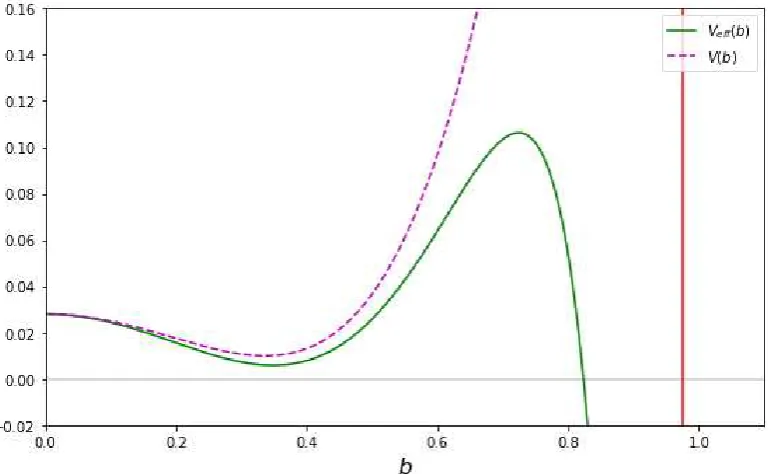
when bothξandΛ_{8are positive, as it is under these conditions that one can most readily construct} models where a positive cosmological constant minimum is present. Figure1shows a specific example of this with parametersΛ_{8 = 0.71, Rd = 0.32 and ξ = 1.64. The dashed (purple) line shows the} potential as it appears in the Friedmann Equation (57), whereas the solid (green) line shows the effective potential (51). Please note that we considerb>_{0 (as the scale factor is positive) and that the}

effective potential is not bounded from below.

Dynamically we expectbto grow from small values and settle down at the minimum of the effective potential. We believe that the effective potential, derived under the assumption that the time–derivatives of the fieldbare negligible, is a good approximation for the case that the fieldbis slowly varying, but a detailed study of the full dynamics ofbis beyond the scope of the paper. Finally we note that the effective mass of the fieldb, given bym2_=Vd=4

eff,bbevaluated at the minimum, is much

larger than the expansion rateH, given by Equation (40), as it should. For the values given in Figure1, we findm/H≈30 at the minimum.

Figure 1.The effective potential (solid line) and bare potential (dashed line) for the parameter choice Λ

8=0.71,Rd=0.32 andξ=1.64 withd=4. The red line on the right shows the limiting values for bfor which the argument in the logarithmic term in the expression for the effective potential (51) is positive. Hence, in all realistic situations, the value ofbwill vary between these extreme values.

3.3.5. Case ofd=5

3.4. Inclusion of Matter

So far we have considered a higher dimensional theory of gravity containing quadratic curvature scalars which reduces to a scalar-tensor theory in 4D. Effects resulting from the presence of matter fields in addition to this have been neglected, and while they are beyond the main scope of this work, we will briefly consider them here. First, by directly adding a minimally-coupled (for simplicity) matter term dependent on both coordinatesxandyto Equation (1),

S= M

2+d

4+d

2

Z

d(4+d)X√₋GR+c1R2+c2RABRAB+c3RABCDRABCD−2Λ4+d+Lm(x,y)

, (58)

we immediately come across a problem in the dimensional reduction procedure in that the integrating-out ofy-dependent terms can no longer proceed fully. Instead we find

S= α

2

Z

d4xp

−gbdL4D+

M2+₄₊d_d

2

Z

d4xddyq₋g(x)qγ(y)b(x)dLm(x,y), , (59)

such that the mixedxandydependencies of the matter Lagrangian prevent further simplification in the absence of an ansatz further specifying the nature of the matter such asLm=Lχ(x)δ(y−y0)where

δis the Dirac delta function. Proceeding with this ansatz, the procedure of dimensional reduction and identification with a Horndeski theory as in Section2.1would then yield an action

S= α

2

Z

d4xp

−ghLH+C0bdLχ i

, (60)

whereC0is a constant given by

C0=

R

ddy√γ δ(y−y0)

R

dd_y√_γ . (61)

The 4D effective action then contains x-dependent matter in the form of χ fields with a non-minimal coupling to the Horndeski fieldb. This implies that our scalar-tensor theory is written in the “Einstein” Frame where the energy momentum tensor associated with theχfields is not covariantly conserved due to explicit interaction with the scalar. That is, variation of the above action gives

Tµν=Tµν(b)+Tµν(χ¯)

=Tµν(b)+C0bdTµν(χ), (62)

whereTµν(χ¯)=C0bdTµν(χ)is a re-defined energy-momentum tensor which, by total energy-momentum conservation, must obey

∇µ_T(b)

µν =−∇µT( ¯ χ)

µν =Qν. (63)

The bare energy-momentum tensor forχhowever is independent ofband only interacts with it via rescaling by a factor ofC0bd. We would expect that

∇µTµν(χ)=0 . (64)

Combining this with the explicit covariant differentiation ofTµν(χ¯):

∇µ_T(χ¯)

µν =C0bd

∇µ_T(χ) µν

+dC0bd−1(∇µb)Tµν(χ), (65)

we would conclude thatQν=dC0bd−1b,µTµν(χ). The equation of motion forbthen take the form

In a cosmological background, where the left-hand side produces the usual Klein-Gordon equation terms (whose particular forms are well documented for Horndeski theories), this means that the right-hand side of the equation of motion forbwould be not zero, but instead

˙

ρb+3H(ρb+pb) =−dC0bd−1b˙ρχ, (67)

while the energy density of the matter field would obey the usual fluid equation

˙

ρχ+3H(ρχ+pχ) =0 , (68)

and the rescaled matter energy density corresponding to the energy-momentum tensorTµν(χ¯) via covariant conservation would obey

˙

ρχ¯+3H(ρχ¯+pχ¯) =dC0bd−1b˙ρχ =d ˙

b

bρχ¯, (69)

where the second equality usesTµν(χ¯)=C0bdTµν(χ)to rewrite the interaction term also in terms of the ¯χ picture. What we see from these calculations is that the presence of matter would in general affect the dynamics of the extra-dimensional scale factor in this theory. As this effect is dependent on the model of the matter fields, including the possibility of more complicated effects arising from non-minimal coupling in the(4+d)-dimensional action, we will neglect its presence in the name of simplicity (the bare field theory already contains 6 free parameters) and model independence (not having results depend on a specific realisation of matter) but at the cost of generality. This means our results will only strictly be applicable to situations in which the matter term in Equation (67) is negligible. The inclusion of matter will, however, influence the location of any effective potential minima as well as potentially alter the dynamics of the system which determine whether such minima are in practice reached from physically useful initial conditions or not. We leave an in-depth look at these possibilities for the future, emphasising that the purpose of the present work is to assess the initial feasibility of this theory first in the simplest available context and in turn provide a starting point for a future work which does systematically consider matter interactions.

A further complication to inclusion of matter which is not as immediate as the dynamical effects, particularly if we were to consider a non-minimal matter coupling in the(4+d)-dimensional action, is that one would have to take into account the point that the conformal rescaling of the metricG

would alter the meaning of the functionb. In particular, a constantbin one conformal frame does not necessarily mean a constantbin other frames, and one would have to be careful when defining things like “static” extra dimensions to specify in which frame they are static and what the physical meaning of this is. On the other hand, if one were to conformally transform a 4D effective action such as Equation (60) to remove the matter-scalar coupling, one would only have to conformally rescale the metricgto achieve this, not the full metricG, leavingb(t)unaltered from its original definition, so it may be possible to avoid such complications.

4. Conclusions

In this paper, we considered a gravitational action in(4+d)dimensions containing the usual Einstein-Hilbert and cosmological constant terms as well as the squares of the Ricci scalar and the Ricci and Riemann tensors with arbitrary constant coefficients. By invoking an ansatz that the metric is the product of a normal four-dimensional metricg(x)and a maximally-symmetricd-dimensional metric

A special case of our results is found when the coefficients of the quadratic curvature scalars in the full action are in the famous Gauss-Bonnet ratio. This combination uniquely leads to a 4D effective action which is a Horndeski theory, albeit with highly non-trivial potentials. A corollary of this is that even arguably-simpler theories like StarobinskyR2gravity in(4+d)dimensions do not correspond to Horndeski-class scalar tensor theories in 4D. As the most interesting and simple possibility, we proceeded to focus on this special case.

In the absence of matter fields, we asked the question of whether the effective potential of the fieldbpossesses a minimum. That is, does there exist a point at which the extra dimensions could stabilise? We further impose the requirement that at such a stable point, if it exists, the effective 4D cosmological constant should be positive-definite. The feasibility of this depends on the number of extra dimensions, and the signs and values of the bare cosmological constant, the Gauss-Bonnet coupling and the extra-dimensional curvature. The casesd =4 andd =5 are the most promising, withd=4 in particular being mathematically more easily handled, and so we focus particularly on this example here, showing that with positive extra-dimensional curvature and appropriately sizes of other parameters, one can find examples where a positive-Λ_{minimum exists. Meanwhiled=1 and}

d=2 are mostly trivial and unable to reliably stabilise,d=3 can only sustain negative-Λ_solutions, andd≥6 may be able to produce desirable solutions with the caveat that they will be unavoidably metastable at best.

We then briefly discussed the issue of including a matter term in the full theory. We studied briefly a toy model of matter which possesses only delta function dependence ony, thus isolating the matter to a single 4D hypersurface, and proceeded to derive the fluid equations for the scalar fieldb

and the matter density in this scenario. While a more realistic treatment of matter fields are needed and should be pursued in future work, it is clear that the details of any matter coupling will affect our results, but there is too much freedom in how this is done to conduct a comprehensive investigation of the possibilities at this stage.

While we have investigated the question of whether stable points can even exist in this theory, we have not answered the accompanying question of whether such a stable point is dynamically approached or not from realistic or generic initial conditions. A future dynamical system analysis, with a reasonable treatment of matter, is left to future work (see [23,24,33] for work in this direction). Given the results from GW170817, indicating that gravitational waves propagate with the speed of light, we believe that the effective theory presented here is relevant only for models of the very early universe. It would therefore also be important to study whether inflation, driven by the fieldb, is viable. It would be also important to study whether inflation, driven by the fieldb, is a viable option. Here, however, our initial results provide a promising starting point, motivating this future work and justifying the time and effort that would need to be spent on this endeavour, given the complexity of the system. It is interesting to note that diverse constraints are needed to be fulfilled: as a model for inflation, it needs to predict the right properties of the primordial power spectrum. In addition, the existence of minima in the effective potential (see e.g., Equation (55) for the cased=4) will provide an additional constraint to be fulfilled by the theory.

Author Contributions:The project was conceptualized by C.v.d.B. The analytical calculations were performed by C.L., using the software Mathematica. Numerical calculations were performed by C.L. using Python. The results were analysed by both authors. The paper was prepared, written and revised by both authors.

Funding: This research received funding by STFC (C.v.d.B. is supported (in part) by the Lancaster-Manchester-Sheffield Consortium for Fundamental Physics under STFC grant: ST/L000520/1; C.L. was supported by an STFC studentship and was supervised by C.v.d.B.)

Appendix A. Proof That the Gauss-Bonnet Combination Is the Only Choice of Coefficients Leading to a Horndeski Theory

Many terms in the 4D effective action such as those proportional to (b) are always Horndeski-allowed, but other terms share a common prefactor, or must have a prefactor that is a derivative of another term’s in order for higher derivative parts to cancel out in the equations of motion. Particularly, this pertains to theG4section of the Horndeski action

LH ⊃G4(b,X)R+G4,X

h

(b)2−(∇α∇βb)(∇α∇βb) i

. (A1)

We equate this with the pertinent terms in 4D effective action derived in Section 2to find conditions on thecncoefficients such that Horndeski form is achieved. Without loss of generality, we takec2=Ac1andc3=Bc1. If the result is to be a Horndeski theory, then there should be a solution forAandB. Proceeding, we conclude by equating theR-proportional part of (6) to that of Horndeski’s action that

G4=1+2c1

Rd b2 +4c1

d(d−1)

b2 X, (A2)

and by equating the terms in (9) with theG4Xterm in Horndeski’s theory, we find the two equalities

G4X = d(

4dc1+c2)

b2 =−

d(dc2+4c3)

b2 . (A3)

Differentiating (A2) with respect toXand equating it to the first expression in (A3) yields

4d(d−1)

b2 =

d(4d+A)

b2 → A=−4 . (A4)

Substituting this result forAinto (A3) then yields

d(4d−4)

b2 =−

d(−4d+4B)

b2 → B=1 . (A5)

Hencec1=c3=−c2/4 and this is the unique solution to the above system of equations, proving that only a constant multiple of the Gauss-Bonnet combination of quadratic curvature scalars will lead to a Horndeski theory in the 4D effective action.

References

1. Zumino, B. Gravity Theories in More Than Four-Dimensions.Phys. Rept.1986,137, 109. [CrossRef] 2. Overduin, J.M.; Wesson, P.S. Kaluza-Klein gravity.Phys. Rept.1997,283, 303–380. [CrossRef]

3. Rubakov, V.A. Large and infinite extra dimensions: An Introduction.Phys. Usp.2001,44, 871–893. [CrossRef] 4. Brax, P.; van de Bruck, C. Cosmology and brane worlds: A Review. Class. Quantum Gravity2003,

20, R201–R232. [CrossRef]

5. Kanti, P.; Gannouji, R.; Dadhich, N. Gauss-Bonnet Inflation.Phys. Rev.2015,D92, 041302. [CrossRef] 6. Wongjun, P. Casimir Dark Energy, Stabilization of the Extra Dimensions and Gauss-Bonnet Term.Eur. Phys. J.

2015,C75, 6. [CrossRef]

7. Nojiri, S.; Odintsov, S.D.; Sasaki, M. Gauss-Bonnet dark energy.Phys. Rev.2005,D71, 123509. [CrossRef] 8. Amendola, L.; Charmousis, C.; Davis, S.C. Constraints on Gauss-Bonnet gravity in dark energy cosmologies.

J. Cosmol. Astropart. Phys.2006,2006, 020. [CrossRef]

9. Amendola, L.; Charmousis, C.; Davis, S.C. Solar System Constraints on Gauss-Bonnet Mediated Dark Energy.

J. Cosmol. Astropart. Phys.2007,2007, 004. [CrossRef]

10. Koivisto, T.; Mota, D.F. Gauss-Bonnet Quintessence: Background Evolution, Large Scale Structure and Cosmological Constraints.Phys. Rev.2007,D75, 023518. [CrossRef]

12. Leith, B.M.; Neupane, I.P. Gauss-Bonnet cosmologies: Crossing the phantom divide and the transition from matter dominance to dark energy.J. Cosmol. Astropart. Phys.2007,2007, 019. [CrossRef]

13. Odintsov, S.D.; Oikonomou, V.K. Viable Inflation in Scalar-Gauss-Bonnet Gravity and Reconstruction from Observational Indices.Phys. Rev.2018,D98, 044039. [CrossRef]

14. Carroll, S.M.; Geddes, J.; Hoffman, M.B.; Wald, R.M. Classical stabilization of homogeneous extra dimensions.Phys. Rev.2002,D66, 024036. [CrossRef]

15. Garraffo, C.; Giribet, G. The Lovelock Black Holes.Mod. Phys. Lett.2008,A23, 1801–1818. [CrossRef] 16. Van de Bruck, C.; Longden, C. Higgs Inflation with a Gauss-Bonnet term in the Jordan Frame.Phys. Rev.

2016,D93, 063519. [CrossRef]

17. Van de Bruck, C.; Dimopoulos, K.; Longden, C. Reheating in Gauss-Bonnet-coupled inflation.Phys. Rev.

2016,D94, 023506. [CrossRef]

18. Van de Bruck, C.; Dimopoulos, K.; Longden, C.; Owen, C. Gauss-Bonnet-coupled Quintessential Inflation.

arXiv2017, arXiv:1707.06839.

19. Alberghi, G.L.; Tronconi, A. Gauss-Bonnet brane cosmology with radion stabilization.Phys. Rev.2006,D73, 027702. [CrossRef]

20. Charmousis, C.; Dufaux, J.-F. General Gauss-Bonnet brane cosmology. Class. Quantum Gravity2002,

19, 4671–4682. [CrossRef]

21. Charmousis, C.; Davis, S.C.; Dufaux, J.-F. Scalar brane backgrounds in higher order curvature gravity.

J. High Energy Phys.2003,2003, 029. [CrossRef]

22. Elizalde, E.; Makarenko, A.N.; Obukhov, V.V.; Osetrin, K.E.; Filippov, A.E. Stationary vs. singular points in an accelerating FRW cosmology derived from six-dimensional Einstein-Gauss-Bonnet gravity.Phys. Lett.

2007,B644, 1–6. [CrossRef]

23. Canfora, F.; Giacomini, A.; Pavluchenko, S.A. Dynamical compactification in Einstein-Gauss-Bonnet gravity from geometric frustration.Phys. Rev.2013,D88, 064044. [CrossRef]

24. Canfora, F.; Giacomini, A.; Pavluchenko, S.A. Cosmological dynamics in higher-dimensional Einstein-Gauss-Bonnet gravity.Gen. Relat. Gravity2014,46, 1805. [CrossRef]

25. Abbott, B.P.; Abbott, R.; Abbott, T.D.; Acernese, F.; Ackley, K.; Adams, C.; Adams, T. Multi-messenger Observations of a Binary Neutron Star Merger.Astrophys. J. Lett.2017,848, L12. [CrossRef]

26. Lombriser, L.; Taylor, A. Breaking a Dark Degeneracy with Gravitational Waves.J. Cosmol. Astropart. Phys.

2016,2016, 031. [CrossRef]

27. Ezquiaga, J.M.; Zumalacarregui, M. Dark Energy After GW170817: Dead Ends and the Road Ahead.

Phys. Rev. Lett.2017,119, 251304. [CrossRef]

28. Creminelli, P.; Vernizzi, F. Dark Energy after GW170817 and GRB170817A.Phys. Rev. Lett.2017,119, 251302. [CrossRef]

29. Sakstein, J.; Jain, B. Implications of the Neutron Star Merger GW170817 for Cosmological Scalar-Tensor Theories.Phys. Rev. Lett.2017,119, 251303. [CrossRef]

30. Zumalacarregui, M.; Garcia-Bellido, J. Transforming gravity: From derivative couplings to matter to second-order scalar-tensor theories beyond the Horndeski Lagrangian. Phys. Rev. 2014, D89, 064046. [CrossRef]

31. Charmousis, C.; Copeland, E.J.; Padilla, A.; Saffin, P.M. Self-tuning and the derivation of a class of scalar-tensor theories.Phys. Rev.2012,D85, 104040. [CrossRef]

32. Kobayashi, T.; Yamaguchi, M.; Yokoyama, J. Generalized G-inflation: Inflation with the most general second-order field equations.Prog. Theor. Phys.2011,126, 511–529. [CrossRef]

33. Pavluchenko, S.A. Cosmological dynamics of spatially flat Einstein-Gauss-Bonnet models in various dimensions: high-dimensionalΛ_{-term case.Eur. Phys. J.2017,C77, 503. [CrossRef]}

c