Generalized construction of trend resistent 2-level split-plot designs

(1)

Rochester Institute of Technology

RIT Scholar Works

Theses Thesis/Dissertation Collections

2-1-2007

Generalized construction of trend resistent 2-level

split-plot designs

Guillermo Lopez

Follow this and additional works at:http://scholarworks.rit.edu/theses

This Thesis is brought to you for free and open access by the Thesis/Dissertation Collections at RIT Scholar Works. It has been accepted for inclusion in Theses by an authorized administrator of RIT Scholar Works. For more information, please [email protected].

Recommended Citation

(2)

G

ENERALIZED

C

ONSTRUCTION OF

T

REND

R

ESISTANT

2-

LEVEL

S

PLIT

-P

LOT

D

ESIGNS

B

Y

G

UILLERMO

L

OPEZ

ATHESIS SUBMITTED IN PARTIAL FULFILLMENT

OF THE REQUIREMENTS FOR THE MASTER OF SCIENCE DEGREE IN

INDUSTRIAL ANDSYSTEMSENGINEERING IN

KATEGLEASONCOLLEGE OFENGINEERING OF

ROCHESTERINSTITUTE OFTECHNOLOGY

INDUSTRIAL ANDSYSTEMSENGINEERINGDEPARTMENT

ROCHESTER, NEWYORK

FEBRUARY2007

COMMITTEEMEMBERS

DR. ANDRESCARRANO DR. BRIANTHORN

ASSOCIATEPROFESSOR ASSOCIATEPROFESSOR

INDUSTRIAL ANDSYSTEMSENGINEERING INDUSTRIAL ANDSYSTEMSENGINEERING

(3)

KATEGLEASONCOLLEGE OFENGINEERING

ROCHESTER, NEWYORK

CERTIFICATE OF APPROVAL

MASTER OF SCIENCE DEGREE THESIS

The M.S. Degree Thesis of Guillermo T. Lopez Perez has been examined and approved by the thesis committee

as satisfactory for the thesis requirement for the Master of Science degree

Dr. Andres Carrano, Ph.D.Advisor

(4)

TO MY FATHER,

WHO HAS GIVEN ME

THE KNOWLEDGE AND SUPPORT

(5)

Abstract

Common experimental practices suggest randomizing the order in which runs are

performed. However, there may be situations in which randomization might not produce

the most desirable order, especially in the presence of known trends. There has been

research done on systematically designing experiments to be robust against trends.

However, few studies address the additional dimensions that arise in nested designs such

as split-plot designs. Split-plot designs have been used for many years in agricultural

applications and are sometimes preferred where there are hard-to-change factors in

industrial settings. There currently is no established methodology to produce split-plot

designs that are robust to potential two-dimensional trends. The objective of this work is

to develop a methodology to design run orders for two-level, split-plot (2w× 2s) designs

that are robust or nearly robust against a set of trends. Two methods are developed in this

work. A fold-over method that uses already established principles is extended for use in

split-plot designs. The second method uses an integer linear programming approach to

search for an optimal design that is resistant to specific trends. A comparison between the

two methods is presented and evaluated with a proposed set of metrics.

Keywords: Split-Plot Experimental Designs, Trend Resistant Run Order, Fold-over,

(6)

List of Figures

Figure 5.1: Arrangement of the runs in a split-plot design ... 21

Figure 5.2: Trends on split-plot designs ... 24

Figure 5.3: Multiplicative interaction between trends. ... 25

Figure 5.4: Additive interaction between trends. ... 26

Figure 6.1: Fold-over on a 22×23split-plot design ... 39

Figure 6.2: Possible combinations for generators in a 2w×22design. ... 41

Figure 7.1: Treatment level combinations used in the ILP ... 54

(10)

List of Tables

Table 3.1: Cake baking experiment ... 11

Table 5.1: Randomly selected run orders for the injection molding experiment... 22

Table 5.2: The linear × linear trend that affects the injection molding experiment... 28

Table 5.3: The linear × quadratic trend that affects the injection molding experiment.... 29

Table 5.4: Trend Index (TI) for each factor ... 31

Table 5.5: Redesigned injection molding experiment ... 32

Table 5.6: Trend indexes (Ti) for each redesigned factor... 33

Table 6.1: TI results for folded generators for 2w × 22split-plot designs for factor A ... 44

Table 6.2: TI results for folded generators for a 22× 23split-plot design ... 47

Table 6.3: Fold-over results for a 22× 23design selected with the TI metric. ... 49

Table 6.4: Fold-over results for a 22× 23design selected with the robust trend metric ... 50

Table 7.1: First stage test run for the ILP model ... 60

Table 7.2: The weights on the trends for stage three ... 61

Table 7.3: Stage 1 results from OPL... 62

Table 7.4: Trend Index for the designs obtained with the ILP method ... 65

Table 7.5: Trend Index for the designs used in stage two ... 67

Table 8.1: Comparison of the Fold-over method and the ILP Method by using the Trend Index ... 70

(11)

Terminology

SPD = Split-Plot Design

DOE = Design of experiments

w= number of factors at the whole-plot level

s= number of factors at the sub-plot level

= denotes the numeric representation of the factor



D = matrix design for the contrast of factor,size: 2w 2s



τ = matrix model for the trend, size: 2w2s

= denotes a specific trend interaction

t= number of trends that the design should be robust against.



N = the total combinatory possibilities for the sub-plot factor

i= position rowion the matrix

j= position columnj on the matrix

k= the treatment level combination (TLC)

TI= Trend Index measurement:



    w s i j j i j i D TI 2 1 2 1 , , ,      j i

c_, = is the contrast level for a factors in rowi and columnj

j i j i c c_, _,

k

V_ = the value of the contrast of factorin permutationk

    otherwise. , 0 . column and row in used is TLC if ,

1 k i j

X_ijk

 



, positivemagnitudetheTIof trend andfactor



s

 



, negativemagnitudetheTIof trend andfactor



(12)

1

Introduction

Experimenters are advised to randomize experiments so that the order of the runs

is not biased; however, there are some situations where it is impossible or simply not

advisable to completely randomize an experiment. Such is the case with blocked,

Latin-squares, nested, and split-plot designs, among others. These situations are called

restricted randomized experiments. These designs impose a restriction that prevents them

from being completely randomized. These restrictions require the experiment to be

analyzed with other methods to provide a significant conclusion.

Sometimes, randomizing the experiment will not produce the most adequate

designs. There is no control over the design when it is done randomly and the sequence

of runs might fall in an undesirable order. On occasions, researchers might be concerned

with possible trends that might affect the results due to an unsatisfying order. Learning

curves, wear and tear, and time-correlated trends are some examples of potentially

damaging trends in experiments. When there are suspicions that a potential trend may

corrupt an experiment, it might be more convenient if the order of the experimental runs

is pre-selected. This will obviously remove the benefits of randomizing the experiments,

but will also reduce the potential for a more damaging trend effect in the results. For this

purpose there are several techniques and strategies that have been studied for the past

decades.

plot designs have been used for many years in industrial applications.

(13)

to change from one treatment over to another. Factors like temperature settings,

machining tool settings, land use or any other factor that requires a large amount of time

to change are considered hard to change factors.

In completely randomized experiments, every treatment combination is positioned

in the experiment in a random order. A split-plot experiment, on the other hand, will

change the hard to change factors less frequently; thus, reducing the time it takes to

perform the experiment.

In the case of split-plot designs, the restriction on the randomization produces a

two-dimensional experiment that could be represented in a row and column procedure

where every treatment in the sub-plots is conducted before changing the treatments in the

whole-plots. There may be potential trend effects across both dimensions; therefore, the

trends that are considered in this thesis are two-dimensional trends. These trends are

composed of a rowcolumn interaction effect between the trends.

This paper will study methods for optimizing a split-plot design to be robust to

various two-dimensional trends. As the experiments become larger, the possible designs

available grow in exponential fashion. If the computer applications need to calculate

every possible outcome, these results can take a large amount of time.

This thesis will concentrate on designing 2k split-plot experiments such that they

are resistant to potential polynomial trends. Furthermore, a fold-over method and an

integer linear programming method will be studied as methods for achieving robust

(14)

2

Problem Statement

Past research on trend resistance has not addressed trends affecting split-plot

experiments. Split-plot experiments robust to trends can be similar to block designs, but

the research done on block designs has only addressed one-dimensional trends while

split-plot designs could potentially be affected by two or more independent trends at the

same time. These independent trends can interact with each other to create a

two-dimensional trend. Unfortunately, very little work has been done on designs affected by

two-dimensional trends.

Many industries today have constraints when performing experiments. Some

experiments tend to be very large and costly. Split-plot designs can considerably reduce

the time of performing an experiment, which in turn will reduce its cost. Past research

suggests that it is better to conduct a split-plot experiment when there are hard-to-change

factors (Lucas and Ju, 1992, and Arvidsson and Gremyr, 2003).

The purpose for this thesis is to design a method for developing 2-level split-plot

experiments that are resistant to potential trends. The possible trends will be identified,

including linear, polynomial, exponential, sinusoidal, and other non-polynomial trends.

Using computer applications such as MATLAB and CPLEX, several designs can be

(15)

3

Background

3.1 Design of Experiments

The purpose of experimentation is to understand the relationship between input

and output variables. By modifying the inputs and recording the changes in the response,

the experimenter can identify what inputs are influential in the response.

Design of Experiments is a set of procedures that are commonly used to conduct

these experiments. Many statisticians have developed methods to conduct experiments

and statistically identify the factors and interactions that are influential in the responses

(Coleman and Montgomery, 1993). One of the more popular methods is called the

Analysis of Variance (ANOVA). The ANOVA is used to identify which factors produce

the greatest changes in the response.

Montgomery describes the single factor statistical model in the book Design and

Analysis of Experiments (2000)as:

  

  

 

n , ... 2, 1,

a , ... 2, 1,

i i

y_ij  _i _ij

whereyijis theijth observation, is the overall mean common to all treatments,i is the

ith treatment effect, ij is a random error component that incorporates all other sources of

variability in the experiment.

This statistical model assumes that the error term,ij, has a normal distribution

(16)

unbiased, the experiment is advised to be designed in a random order. The randomness of

the experiment will reduce the noise effects in the response.

There is a consideration with the size. When performing an experiment, one of the

biggest limitations is cost. In general, the larger the size of the experiment the more

costly it can be. Experimenters always try to reduce the size of the experiment. Running a

fraction of the total number of runs is a method used to reduce the size of the factorial

designs. These designs are called fractional factorial designs. However, this limits and

confounds some responses and the experimenter should take into consideration what was

lost.

On occasions, an experiment could be constrained by time, size, costs, or other

factors. These restrictions produce several situations that require advanced experimental

designs. If the experiment is designed appropriately and every restriction, constraint and

outside influence is taken into consideration in the experiment, then the experiment might

yield more reliable results.

3.2 Trends

Sometimes, randomizing the run order of an experiment might yield an

undesirable order, especially in the presence of a trend. A trend is an uncontrolled

variable that is highly correlated with the experiment, such as learning curves and the

passing of time. This is commonly known as a time trend (Hill, 1960, Steinberg, 1988,

John, 1990, etc), but for the purpose of this thesis, the time trend will be addressed simply

as a trend. Randomizing will help guard against noise variables. Trends, on the other

(17)

When experimenters anticipate that there may be uncontrolled variables in their

experiments, they could choose to ignore them, block them, include them in the

experiment, or conduct the experiment in an order in which these variables do not affect

the results. To be resistant to a particular trend, the experiment should be designed so that

it is orthogonal to the trend.

There are several well-established representations of the trends including that of a

vector with the value of the trend at that position or sequence in the experiment: (1, 2, 3,

4, …, i). This model is referred to as a linear trend because it follows a linear pattern.

Linear trends can be modeled with the following formula:yaxb. Daniel and

Wilcoxon (1966) used a linear polynomial for a 24factorial experiment. In this work, the

trend was modeled as (-15, -13, -11, …, -1, +1, …, +13, +15).

Most experimenters tend to be concerned with linear trends and sometimes with

quadratic trends, but typically not higher. If the contrast and the trend are orthogonal,

then the contrast is considered trend free.

It is known that a contrast with coefficients (₁,₂,...,_n) is orthogonal to a trend

of thekth-order if the response is not correlated, the variance is the same, and they meet

the following condition:

0

1







n

i k ii

 ,

for n experimental runs, where k is the order of the trend. Considering the following

example: a 23 factorial experiment, whose run order is



(1) a b ab c ac bc abc



and a linear trend modeled as:



1 2 3 4 5 6 7 8



is present, the run order will not satisfy the rule: 0

1







n

i k ii

(18)

for any factor. In fact, it will be equal to 4, 8 and 16 for factors A, B and C respectively.

However, if the run order is changed to



c a b abc ab bc ac (1)



, then all

factors will satisfy 0

1







n

i k ii

 . The latter design is considered to be robust against the

trend in question.

Most research in this field considers only polynomial trends. There is a possibility

that a trend might be best modeled as a non-polynomial (Atkinson and Donev, 1996). In

some cases, such as weather patterns, the trend might be modeled as a sinusoidal model,

or an exponential model for elements with a very short half-life or decay function.

3.2.1 Polynomial Trends

A polynomial trend would be modeled by the general equation:

0 1 1 2 2 1

1x ... a x a x a

a x a

y p p

p

p     

 

 wherexis the position of the design point and

yis the effect of the trend. Also,pdenotes the degree of the polynomial.

Experimenters have studied the effects of polynomial trends and the consequences

of the degree of the trend. Linear and quadratic models (p=1 and p=2) are of most

concern among experimenters. Higher order trends might also be of some concern if

found present in the experiment.

There are many other possible trends that could be modeled as a polynomial.

Positional trends, learning curves and tool wear are common trends that an experimenter

(19)

3.2.2 Sinusoidal Trends

Sometimes, the trend of concern might be difficult to model as a polynomial. Any

trend that is suspected to have a cyclical variation is probably best modeled as a

sinusoidal model. These models follow the general sinusoidal equation: yasina0

where θis the radian position of the design point and y is the effect of the trend.

Experiments, especially those that take an extremely large time to conduct, could have

some seasonal changes or uncontrolled temperature fluctuations.

Some possible trends that can be modeled with a sinusoid are seasonal changes,

temperature fluctuations and vibrations.

3.2.3 Exponential Trends

Exponential trends may also be of concern. Wear and decay of materials used,

radioactive half-life, or population changes that could affect certain experiments might

have some effect on the design. These trends can be modeled by variation of the

equation: 0

) (

a a

y  ppx 



where xis the position of the design point andyis the effect of

the trend, andpdenotes the degree of the model.

3.3 Restricted Randomized Experiments

There are situations in which an experiment cannot be completely randomized.

This can be due to limited amounts of space or time. Common restrictions can include

experiments that need to be run at the same time, or when the experimental runs use

several batches of materials, or when there are different operators or equipment for a set

(20)

types of experiment offer valid results for certain restrictions while sacrificing other

information.

By completely randomizing the experiment, the potential effects of noise and

other uncontrolled variables are lessened in the experiment. This advantage may be

discarded because there are other more important considerations in the experiment. It is

common to see an experiment that can be conducted as a completely randomized

experiment, but the experimenter chooses to purposely restrict the randomization so as to

obtain other valuable information or to arrange for a less complicated experiment.

Common restricted randomized experiments are blocked, Latin-squares, nested

and split-plot designs. The blocked designs are used when there are different

environmental or operational conditions between groups of runs in the experiment, such

as: two operators each conducting a part of the experiment or an experiment that takes so

long that parts of the experiment are conducted on different days. It is true that the

experiment can be designed by including the operators as factors in the experiment, thus

reducing this problem; however, the response due to operators in this situation is either

unimportant or fairly obvious. Besides, adding the operators as a new factor, will double

the size of the experiment.

Latin-squares designs are used to block multifactor designs in two directions.

They are mostly used as a mean to reduce the size of very large experiments with factors

that have large number of levels. Latin-squares have very good estimates for the main

effects. There are several variations to the Latin-squares such as incomplete Latin-squares

(21)

Nested designs are used when the factors are in a hierarchy, and the levels of

some factors are nested under the levels of other factors. For example, if an experimenter

wishes to compare different cooking styles from different chefs, each chef uses several

factors that will be considered in the experiment. The problem is that the chefs use

different ingredients and utensils rather than having all the chefs with the same factors.

This difference can be influential in the experiment and cannot be conducted as a

completely randomized experiment, because it might not yield a valid response.

Split-plot is a special case of nested designs and originated in agriculture, when

experimenters wished to perform experiments on the crops. This caused problems

because crops are seasonal and had to be conducted over several years. To avoid this, the

land was separated into several plots and the experimental runs were all conducted at the

same time. This technique allowed experimenters to run the entire experiment in one

season, preventing uncontrolled climatic variables to affect the results. The following

section presents a more detailed explanation of split-plot experiments.

3.4 Split Plot Designs:

Split-plot experiments or SPDs are usually conducted when there are “hard to

change” factors included in the experiment. Hard to change factors are those that, when

compared to the other factors in the experiment, will take a longer time to change from

one setting to another or are just too expensive or resource intensive to change in a

random matter. Temperature changes, complicated and time consuming machine settings,

large batches of materials, plots of croplands, among others are some examples of

(22)

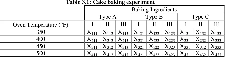
Table 3.1 illustrates a cake baking experiment as an example. The purpose of this

experiment is to test how much a cake would rise with different ingredients and at

specific oven temperatures. In this example, there are three types of baking mixtures that

combine different ingredients at different proportions. The mixtures are prepared and

baked at four different temperature levels in the oven. Three replicates are run under

every treatment combination of temperature and ingredients. This experiment can be

completely randomized by randomly selecting the temperature and the ingredient mix

and performing the experiment at these settings. Afterwards, a new temperature and

mixture is randomly selected, excluding the ones already performed, and the experiment

is run at the new settings.

When hard to change factors are involved, like the temperature in the oven,

randomly selecting the temperature will make this experiment too expensive. Changing

[image:22.612.81.539.434.550.2]

the temperature of the oven on every run of the experiment will make this experiment too

Table 3.1: Cake baking experiment

Baking Ingredients

Type A Type B Type C

Oven Temperature (F) I II III I II III I II III

350 X111 X112 X113 X121 X122 X123 X131 X132 X133

400 X211 X212 X213 X221 X222 X223 X231 X232 X233

450 X311 X312 X313 X321 X322 X323 X331 X312 X333

500 X411 X412 X413 X421 X422 X423 X431 X432 X433

Note: Xijkrepresents data points whereiis the oven temperature,jis the baking ingredient, andkis the replicate.

expensive or impractical. The most convenient and logical way to perform such an

experiment is to set the oven at one temperature (randomly selected) and perform all the

other settings either at the same time inside the oven or one at a time but with the same

temperature setting. For example, the temperature of the oven is heated to 350F and

(23)

introduced in the oven and cooked at 350F. After the cakes are baked, the temperature in

the oven is changed to a new setting (i.e. 400F) and 9 new mixtures are introduced into

the oven. This process is repeated until all temperatures have been tested. The

temperature factor, with its 9 data points, is referred to as the whole-plots, while the

ingredients are referred to as split-plots or sub-plots.

SPDs originated when experimenters had to perform experiments on crops where

they could not use the same plot of land for the experimental contrasts. Currently,

experiments on croplands are designed as split-plot experiments or Latin-squares.

Split-plots have their limitations. Since the hard-to-change factors and the

whole-plots are the same, any condition that changes from one plot to the next may generate as a

temperature effect. This arrangement will have the main effects confounded with the

plots. There is also an extra error term that is included in the whole plots. An appropriate

model for this experiment can be:

ijk ijk ij

jk j

ik i k

ijk R T TR B BR TB TBR

Y        

where R is the replicate, T is the temperature, TR is the Replicate Temperature

interaction, B is the baking ingredients, BR is the Replicate Baking Ingredients

interaction, TB is the Temperature Baking Ingredients interaction, TBR is the

three-way interaction, andis the error term. The TR interaction is considered the whole-plot

error.

3.5 Trends on Two-level Split-Plot Designs

It has come to the attention of some researchers (Edmondson, 1993, Carranoet al,

(24)

experiments, the results might be impacted by a composite, two-dimensional trend effect.

Edmondson called these designs row column designs and that these could be affected

by row column trend interaction. Edmondson (1993) concentrated on Latin-squares

while Carranoet al(2002, 2007) observed a specific split-plot experiment.

Carranoet al(2002) performed a split-plot experiment to determine the effect of a

set of process parameters on the roughness of the wood surface when it is sanded. The

run order of this experiment was systematically planned to be trend resistant. The input of

the experiments were as follows: wood species, grit size, depth of cut, tooling resilience,

feed rate, spindle speed, and grain orientation. Each factor had 2 levels except for the

wood species, which had 3 levels. The size of this experiment was 3126 192

treatment combinations. Changing the parameters randomly between each experimental

unit would have been cost intensive and time consuming. It was decided to perform a

split plot experiment, where the machine parameters were set to be the whole-plot factors

and the wood setup will be the sub-plot factors. In the sub-plot, the wood had 31216

units (species orientation). Then the spindle passed on all 6 units. The machine factors

are varied between runs for a total of 25 32

experimental runs.

This arrangement of the split-plot allowed the reduction of cost and time when the

experiment was performed. There was, however, a concern for the wear of the tool and

particular learning curves when setting up each experiment. It was noted that if they were

to be resistant to these trends, the experimental runs needed to be ordered appropriately.

Carrano et al (2004, 2007) showed the appropriate order for this experiment. They

(25)

they assumed the presence of a trend across the whole-plots. This meant that each

sub-plot trend would be different among the other whole-sub-plots.

In this work, the researchers used the available methods in literature on trend

resistance to find an optimal run-order. Since there is no other research available that

questions the two-dimensional trend, their work establishes the foundation for a general

construction for trend-resistant split-plot designs.

The following thesis particularly addresses the generalization of the work Carrano

et al (2007) performed by finding appropriate designs for two-level trend resistant

(26)

4

Literature Review

4.1 DOE and Nested Designs

When performing an experiment, it is desirable to randomize the order in which

the experiment is conducted. There are, however, situations in which a complete

randomization of the experiment is not feasible or recommended. Costs and time factors

can constrain the experiment making it difficult to completely randomize the experiment.

Whenever the experimenter is unknowledgeable about the experiment, this could lead to

unreliable analysis of the experiment (Coleman and Montgomery, 1993). Techniques for

coping with restrictions to randomization include blocked designs, nested designs and

split-plot designs. Arvidsson and Gremyr (2003) compared how the results are affected if

the experiment is done by completely randomizing the experiment or by deliberately

restricting the runs.

Experimenters routinely encounter experiments in which one or more factors are

very hard or very costly to change. In these cases, it might be more convenient for the

experiment to be analyzed as a split-plot design, which accounts for hard-to-change

factors and easy-to-change factors. A split-plot design is a form of restricting the

randomization of the experiment. Lucas and Ju (1992) point out that analyzing

experiments that contain hard to change factors as if they did not, would not yield the

most desirable results. This is because experiments that have hard-to-change factors often

(27)

factors, could mask the effects of the easy-to-change factors. Therefore, these

experiments should be performed as a split-plot experiment.

4.2 Experimental Designs with Trends

It is possible for experiments to be affected by trend effects. In these cases, when

the experimental units are selected at random, the trends can have undesirable effects in

the results. Cox (1951) discussed the presence of a possible trend in randomized

experiments. It is possible to design the experiment in such a way that the trend effects

are orthogonal to the effects of interest in the experiments. Cox (1951, 1952) produced

design plans that deal with first order trends. Daniel and Wilcoxon (1966) discuss why

experiments should be resistant to trends and suggest a few designs as well. The

consequences of ordering the design points in an experiment have been studied. Atkinson

and Donev (1996) concluded that very little information is lost when the experiment is

designed to be resistant against trends when in fact there is no trend present. Thus, when

the experimenter assumes that there is a possible trend that might affect the result, it may

be convenient if the experiment is robust to the trend. Whether the trend exists or not,

may be irrelevant.

There have been several works that have considered trends when designing

experiments. Daniel and Wilcoxon (1966) have developed plans where some main effects

are robust against quadratic trends. Cheng and Jacroux (1988) developed an algorithm

that generates trend free runs and gives estimates of main and two-factor interaction

effects protected against high-degree polynomial trend effects. Jacroux and Ray (1990)

give a method that constructs the order of experiments that contain v treatments and n

(28)

John (1990) applies the principle of folding over on the experimental runs to

generate runs that are resistant to linear and quadratic time trends. Other works have been

performed on different forms of experiments: Cheng and Steingberg (1991), Baileyet al

(1992), Coster (1993), Jacroux (1994) refer to factorial experiments, Daniel and

Wilcoxon (1966) consider fractional factorial designs, while Jacroux (1996), Steinberg

(1988), and Edmonson (1993) study the effects of the trend itself.

4.3 Split-plot designs and trends

Experimenters have developed techniques to design experiments that are resistant

to possible high-order trend effects; however, little has been done on designing trend

resistant split-plot or other nested designs. Goos and Vandebroek (2004) mention that

these designs naturally give better protection against trends but they do not address the

effects of a trend on these designs.

Blocked designs with trends have received lots of attention in the past twenty

years which originated with Bradley and Yeh (1980). They discuss trend resistance in

blocked designs and why is it important to be resistant to possible trends. Yeh and

Bradley (1983, 1985) have developed methods for constructing trend-free and nearly

trend-free block designs. Stufken (1988) studied trend-free block designs, and concluded

that there are some criteria that will prevent an experiment from being trend-free. In this

paper, Stufken mentions the parameters that a block design should have to be resistant to

possible trends. Other works concerning block designs include: Lin and Dean (1991),

Chai and Stufken (1999), Lin and Stufken (1999, 2002), and Tack and Vandebroek

(29)

Box and Jones (1992) compare methods of performing experiments when some

environmental condition arises that can affect the results. They compare completely

randomized, split-plot and strip-block experiments. They have concluded that split plot

designs that take these environmental issues into account are very reliable. The

environmental conditions used by Box and Jones are known effects and were introduced

into the experiment as hard-to-change factors, but trends may have unknown effects on

the factors and cannot be modeled like this experiment. Kowalski (2002) is concerned

with split-plot experiments robust to parameter designs and uses a form of semi-folding

to generate 24 run experiments for this purpose.

Carranoet al(2002) performed a split-plot experiment on wood machinery where

the settings for the machine were set as the whole-plot factors and the type of wood and

grain orientation were set as the sub-plot factors. Suspecting that there could be a

possible unknown trend effect due to time and position, the experiment was designed to

be robust against two linear trend effects. By combining the technique used by Daniel

and Wilcoxon (1966), the principle of folding over and a nonlinear integer program, they

developed a feasible design that would be simultaneously resistant to two linear trends,

one for the whole-plots and the other for the sub-plots.

For any split-plot design the experimenter may have several factors that are hard

to change at a whole-plot level, and some factors that are easy to change, and are located

in a sub-plot level. There is also the potential existence of individual trends, some for the

hard to change factors and others to the easy to change factors. Edmondson (1993)

considered that row-and-column designs are affected by a row column interaction

(30)

to assume that they could be affected by a two-dimensional trend. Atkinson and Donev

(1996) mentioned that the trend might not be accurately modeled as a polynomial.

Depending on the environmental conditions, the trend might be better represented as an

exponential or sinusoidal model instead. There has been little work that considers these

trends. Steinberg (1988) modeled some time trends as an autoregressive integrated

moving average (ARIMA) time series and shows how this can be helpful in factorial

experiments. Still, works on exponential and sinusoidal models are missing.

Split-plot experiments are widely used in industrial environments. Protecting

against possible trends will enable these experiments to give unbiased results. Most

research on similar experiments only considers trends modeled by a one-dimensional

array across all runs. The purpose of this work is to propose a method to design split-plot

experiments that are resistant to two-dimensional trends. As shown in this section, this

(31)

5

Methodology

5.1 The Split-Plot Model

In order to simplify calculations when designing a trend resistant split-plot

experiment, a matrix format with rows and columns is followed in this work. The rows

will represent the whole-plot treatments and the sub-plot treatments will be arranged

along the columns. Each cell in the matrix contains the treatment level combination of all

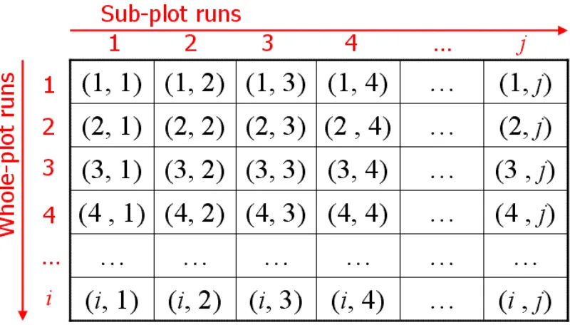
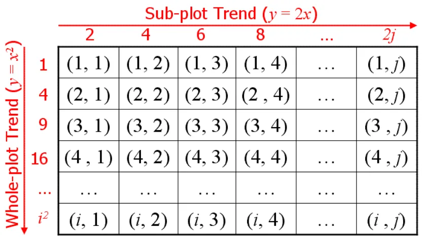
the factors in that run of the experiment. Figure 5.1 shows how the runs are arranged in a

split-plot experiment. The experimenter will set the whole-plots at the desired level in the

ith row and run accordingly all the sub-plot runs within that row across the columns. The

split-plot design has a 2w2ssize (i.e. number of treatment level combinations) wherew

is the number of factors at the whole-plot level and sis the number of factors at the

sub-plot level. The matrix Dis defined such that it will have 2w rows and 2s columns and represents the contrast matrix of factor . Each unit in Dwill represent the level of factor at that point (i.e. treatment) in the experiment. The way split-plot designs are

typically conducted, the first experimental unit will be the treatment level on the 1st

column in the 1strow. The second treatment will be on the 2ndcolumn in the 1strow, and

so forth until there are no more experiments to be run in that 1st row. This completes all

the runs for the whole-plot represented in the first row. The next run will begin in the 1st

column on the 2nd row, and so on until all rows and columns have been done. To better

illustrate these notations, the following injection-molding experiment will be used

(32)

[image:32.612.106.506.79.307.2]

Figure 5.1: Arrangement of the runs in a split-plot design

5.1.1 The Injection Molding Experiment

In an injection-molding experiment, where the factors considered include: A)

barrel temperature, B) mold temperature, C) holding pressure, D) back pressure and E)

injection speed. This experiment has 5 factors at 2 levels. Typically for this type of

experiment, the temperature settings are considered hard to change because every time

the setting is changed, the temperature has to be reset and increased or decreased to the

desired temperature. These heating and cooling cycles can be very time consuming. If

conducted as a 25 fully randomized factorial experiment, this could require far more than

several days of experimentation. Additionally, this may expose the system to the effects

of nuisance factors that cannot be controlled, or even worse, factors that the experimenter

might not be aware of. For experiments like these that involve hard-to-change factors, it

(33)

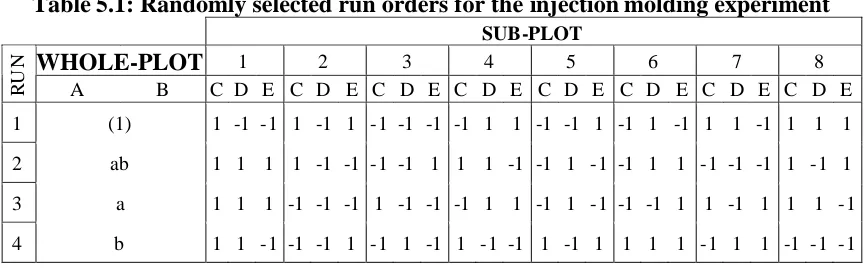
For this example, factors A (barrel temperature) and B (mold temperature) are

considered as the whole-plot factors while C (holding pressure), D (back pressure) and E

(injection speed) are the sub-plot factors. A random order is selected and shown in Table

5.1. As shown in the table, factors A and B are set at their low level (-1) in the first row.

Afterwards, within the same run, the sub-plot factors are changed and run eight times

(23), which is the total number of treatment level combinations. The first whole plot or

row 1, is: c, ce, (1), de, e, d, cd and cde. After performing the first whole-plot run, the

whole-plot treatments are set to ab and the runs are: abcde, abc, abe, abcd, abd, abde, ab,

and abce. The experiment will continue in the same fashion by changing the

hard-to-change factors just when all the treatment combinations of the subplot factors are

[image:33.612.90.523.381.515.2]

exhausted.

Table 5.1: Randomly selected run orders for the injection molding experiment

SUB-PLOT

WHOLE-PLOT 1 2 3 4 5 6 7 8

R

U

N

A B C D E C D E C D E C D E C D E C D E C D E C D E

1 (1) 1 -1 -1 1 -1 1 -1 -1 -1 -1 1 1 -1 -1 1 -1 1 -1 1 1 -1 1 1 1

2 ab 1 1 1 1 -1 -1 -1 -1 1 1 1 -1 -1 1 -1 -1 1 1 -1 -1 -1 1 -1 1

3 a 1 1 1 -1 -1 -1 1 -1 -1 -1 1 1 -1 1 -1 -1 -1 1 1 -1 1 1 1 -1

4 b 1 1 -1 -1 -1 1 -1 1 -1 1 -1 -1 1 -1 1 1 1 1 -1 1 1 -1 -1 -1

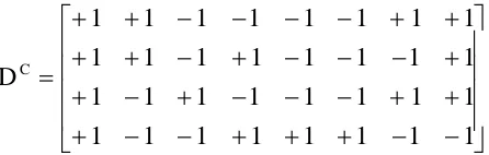
In this example, the design matrix for the whole-plot factor A is:

(34)

While the design matrix for the sub-plot factor C is:                                              1 1 1 1 1 1 1 1 1 1 1 1 1 1 1 1 1 1 1 1 1 1 1 1 1 1 1 1 1 1 1 1 DC

and similarly for the other factors.

5.2 Two-dimensional Trends

When looking at possible trends that can affect a split-plot design, the sub-plot

factors might have a trend that runs across them. In the same manner, the whole-plot

effects could also be affected by another possible trend. These column and row trend

effects, if present, may have a composite effect in the experiment.

[image:34.612.131.354.100.171.2]

5.2.1 Trend Presence on the Sub-plot

Figure 5.2 shows how a split-plot arrangement can be affected by a trend. This

trend, called the plot trend in this work, could be present while conducting the

sub-plot runs. This trend could be present and repeats itself every time the sub-sub-plots are run.

When the first sub-plot is run in the experiment, there could be a linear time trend (i.e.:

x

y2 ), as shown in Figure 5.2. This will mean that the first treatment combination in

the first run (i.e.: 1,1) will experience an effect of magnitude 2. Similarly the next

experimental unit will have a trend effect of magnitude 4, the third will be 6 and so forth

until all runs are done. When performing the next run (i.e.: 2,1 2,2 … 2,8), the first will

(35)

5.2.2 Trend Presence on the Whole-plots

Just like the sub-plot runs, each whole plot run could be contaminated by a trend

referred to as a plot trend. The split-plot arrangement in Figure 5.2 has a

whole-plot trend (i.e.: 2

x

y  ) as well as a sub-plot trend (i.e.: y2x). This will mean that the

first whole-plot run might be affected differently than the second and third whole-plot

treatment combination. While each whole-plot run is affected by the same sub-plot trend,

this gets compounded or amplified by the whole-plot trend. This means that the second

sub-plot treatment combination in the first whole-plot row might not be affected in the

same way as the second sub-plot in the second whole-plot row. This last statement forms

[image:35.612.99.515.358.593.2]

the basis for the hypothesis tested in this thesis.

Figure 5.2: Trends on split-plot designs

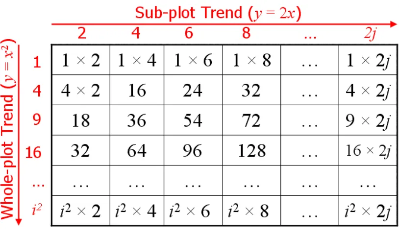
5.2.3 Trend Interaction

As mentioned before, the whole-plot trend will have an effect on each sub-plot

(36)

defined as the value of the interaction between a whole-plot trend and a sub-plot trend on

the ith row and the jth column. This interaction can be modeled mathematically by

making some assumptions.

A multiplicative interaction, as shown in Figure 5.3, will multiply the value of

each whole-plot and the sub-plot trends. The example assumes that the sub-plot trend is

modeled as y2x while the whole-plot trend is quadratic modeled as 2

x

y  . The

effects of the trend show a multiplicative increase in the effects of the trends. Therefore,

2 , 1

[image:36.612.102.509.303.543.2]

 has a value of 4 while2,2 has a value of 16.

Figure 5.3: Multiplicative interaction between trends.

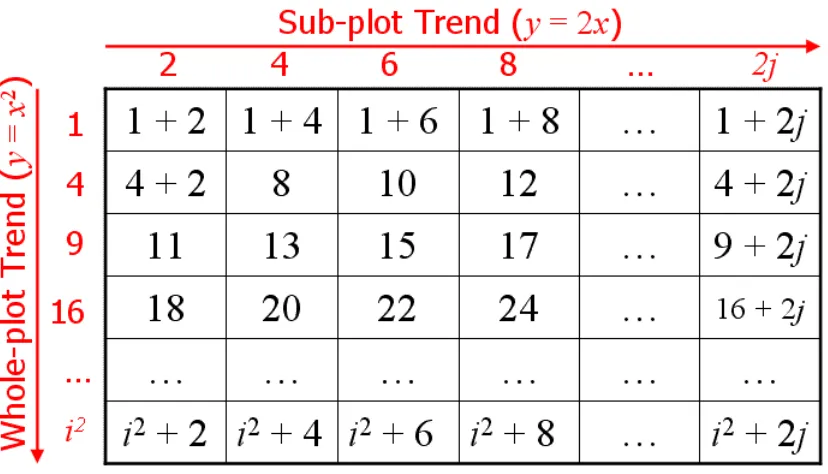
Figure 5.4 shows an additive interaction between the whole-plot trend and the

sub-plot trend. The additive interaction assumes that there is equal spacing between the

runs, while in the multiplicative interaction, the difference between 2,2 and 2,3 is

(37)

interaction. By using the additive interaction it is implied that the spacing between runs

has the same interval through time or position.

A subtractive interaction is a form of adding negative numbers; therefore, the

additive interaction will work for this interaction. Just like subtraction, division is the

multiplication of fractional numbers and they can also be interpreted as a multiplication

[image:37.612.101.515.241.478.2]

interaction.

Figure 5.4: Additive interaction between trends.

5.2.4 Implications from ignoring two-dimensional trend

Two-dimensional trends assume that there could be a trend that is correlated to

the whole-plots. If this assumption is ignored, then it is implied that every whole-plot

treatment combination is conducted under the exact same conditions. If this were the

case, then there would be no two-dimensional trends in the split-plot and the whole plot

factors can be selected randomly. However, there are situations where exact experimental

(38)

onsite in a manufacturing plant or outdoors with unpredictable climate conditions. In

these cases, trends that might be present on the whole-plots will also be present on the

sub-plots by interacting with the sub-plot trends.

As shown in section 5.2.3, each sub-plot could have a different trend due to the

multiplication or addition of the whole-plot trend. If this interaction is ignored, a

systematic selection of the run order might result in a design that is robust to the

one-dimensional sub-plot trend or to the one-one-dimensional whole plot trend, but it might not be

robust to the two-dimensional trend, resulting in a design that may adversely affect the

results of the experiment.

5.2.5 Multiple 2D trends

There could be more than one trend that affects the whole-plot and sub-plots. The

number of trends that could be modeled is infinite because the parameters in the models

for trends can be modified in many ways to incorporate these.

Most of the possible trends are of no concern to the experimenter either because

their potential correlation is insignificant compared to the few important trends. The

trends that the experiment needs to be robust against are those that are suspected to have

the highest influence in the design. It could be either 2 or 20 trends at the discretion of the

experimenter. An experimenter might consider that if a trend could affect the experiment,

then it may be worthwhile to design against it.

Being robust against the greatest number of potential trends may be the best

option. Unfortunately, the more trends the design is supposed to be robust against, the

(39)

5.2.6 Example

The injection molding example before might be affected by various trends.

Consider that the sub-plot could be affected by the following polynomial trends modeled

as yxand 2

x

y . Furthermore a possible polynomial trend might be present on the

whole-plots. Combined with the column trend, the resulting trend that affects the design

could be an interaction between these two trends. This interaction can vary depending on

how the whole plot trend interacts with the sub-plot trend.

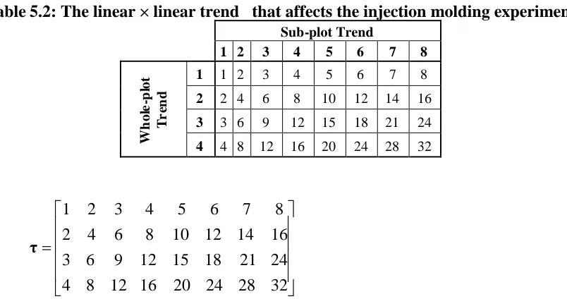
Consider the example in Table 5.2, where the whole-plots and the sub-plots have

linear trends, and the interaction between the linear whole-plot trend and the linear

sub-plot trend is the multiplicative between them, where i,j ij and will produce the

[image:39.612.107.509.388.600.2]

following linear × linear trend represented by the matrix τ:

Table 5.2: The linear × linear trend that affects the injection molding experiment

Sub-plot Trend

1 2 3 4 5 6 7 8

1 1 2 3 4 5 6 7 8

2 2 4 6 8 10 12 14 16

3 3 6 9 12 15 18 21 24

W h o le -p lo t T r en d

4 4 8 12 16 20 24 28 32

             32 28 24 20 16 12 8 4 24 21 18 15 12 9 6 3 16 14 12 10 8 6 4 2 8 7 6 5 4 3 2 1 τ

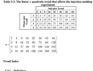
In table 5.3, the sub-plots are now believed to be affected by a quadratic trend and

with the same multiplicative interaction between the linear whole-plot trend and the

quadratic sub-plot trend. Therefore i,j ij2 resulting in the following linear ×

(40)

[image:40.612.105.495.73.371.2]

Table 5.3: The linear × quadratic trend that affects the injection molding experiment

Sub-plot Trend

1 4 9 16 25 36 42 64

1 1 4 9 16 25 36 42 64

2 2 8 18 32 50 72 84 128

3 3 12 27 48 75 108 126 192

W h o le -p lo t T re n d

4 4 16 36 64 100 144 168 256

             256 168 144 100 64 36 16 4 192 126 108 75 48 27 12 3 128 84 72 50 32 18 8 2 64 42 36 25 16 9 4 1 τ

5.3 Trend Index

5.3.1 Definition

In this thesis, the robustness of a design against the trends will be measured by

calculating the proposed Trend Index (TI). The Trend Index proposed in this work is a

measurement of how robust the design is against a specific trend. More specifically, it

cumulatively measures if a trend has an adverse effect on a particular design. Draper and

Stoneman (1968), and Dickinson (1973) refer to this term as a time count but this is

probably because they studied the robustness against time-correlated variables. The

Trend Index defines a much broader area of robustness and assumes that the trends do not

necessarily have to be time related. Instead, there could be many types of trends such as

learning curves, tool wear, and temperature fluctuations as mentioned in section 3.2.

A value of 0 on the TI will define that the selected design is perfectly orthogonal

(41)

a specific design and trends should not be compared to other designs and trends of

different size in dimensions. The TI is a measurement that compares the robustness of a

particular design against one or more trends with other arrangements of the same

experiment.

The proposed TI can be used in calculating the robustness of any design of any

dimension. This thesis will focus on the TI with two-dimensional trends from hierarchical

designs such as split plots.

5.3.2 Notation

Let Dbe the design matrix of contrast for factor and τbe the matrix that denotes a trend with the same size as D. The formula used to measure the robustness of the design is:



    w s i j j i j i D TI 2 1 2 1 , ,    .

This TI will be used to quantify the robustness of the contrast arrangement of factor 

with the trend τ. It is convenient to standardize the TI so that it will always show a

positive value. This helps when comparing trend indexes and optimizing the design. To

incorporate more than one two-dimensional trend, a set of τ_ is defined where 

represents a specific trend interaction as defined by the experimenter. With the addition

of the new trends, the formula is modified to:



    w s i j j i j i D TI 2 1 2 1 , , ,     

(42)

5.3.3 Example

Using the injection molding experiment introduced in section 5.1 and the trends

obtained in section 5.2, the experiment needs to be simultaneously robust against the

following two trends:

             32 28 24 20 16 12 8 4 24 21 18 15 12 9 6 3 16 14 12 10 8 6 4 2 8 7 6 5 4 3 2 1 1

τ , and

             256 168 144 100 64 36 16 4 192 126 108 75 48 27 12 3 128 84 72 50 32 18 8 2 64 42 36 25 16 9 4 1 2 τ

Where τ₁ is produced by the following model:_i_,_j ij, and τ₂ is produced by the

model: 2

,j i j

i 

[image:42.612.127.353.189.347.2]

 .

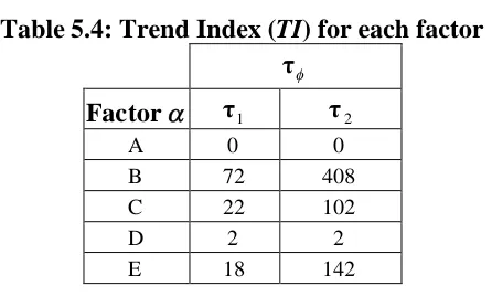
Table 5.4 gives the trend indexes of all five factors in the run order established in

section 5.1.1. Only factor A is resistant to both trends.

Table 5.4: Trend Index (TI) for each factor

 τ

Factor τ1 τ2

A 0 0

B 72 408

C 22 102

D 2 2

E 18 142

The random selection did not produce trend resistance on the other factors. For

[image:42.612.196.419.479.613.2]

(43)

                                             1 1 1 1 1 1 1 1 1 1 1 1 1 1 1 1 1 1 1 1 1 1 1 1 1 1 1 1 1 1 1 1 DC

in the injection molding experiment yielded the following trend indexes:

22 4 1 8 1 1 , , C , C

1 



 

  i j j i j i D

TI  for τ1 and 102

4 1 8 1 2 , , C , C

2 



 

  i j j i j i D

TI  for τ2.

Factor C is not robust to either τ1 or τ2.

[image:43.612.127.351.72.143.2]

If the design for the injection molding experiment is modified as proposed on

table 5.5 then the trend index will change as seen on table 5.6. Every sub-plot factor has

received a substantial improvement. The linear sub-plot trend has no effect on factor B.

To improve the robustness of factor B will require the reordering of the whole-plot

factors, which might aggravate factor A. It is up to the experimenter to decide what

design is best for the whole-plot factors. The order of the whole-plot factors will not have

any negative effect on the trend index of the sub-plot factors. Therefore run orders for the

[image:43.612.93.468.185.230.2]

subplot factors and the whole-plot factors can be designed separately.

Table 5.5: Redesigned injection molding experiment

SUB-PLOT

WHOLE-PLOT 1 2 3 4 5 6 7 8

R

U

N

A B C D E C D E C D E C D E C D E C D E C D E C D E

1 (1) -1 -1 -1 1 -1 -1 -1 1 -1 1 1 -1 -1 -1 1 1 -1 1 -1 1 1 1 1 1

2 ab 1 1 1 -1 1 1 1 -1 1 -1 -1 1 1 1 -1 -1 1 -1 1 -1 -1 -1 -1 -1

3 a 1 1 1 -1 1 1 1 -1 1 -1 -1 1 1 1 -1 -1 1 -1 1 -1 -1 -1 -1 -1

(44)

[image:44.612.171.451.77.200.2]

Table 5.6: Trend indexes (Ti) for each redesigned factor

 τ

Factor τ1 τ2

A 0 0

B 72 408

C 0 0

D 0 0

E 0 0

Comparing the results of both designs, the second design contains four factors

that are robust to τ1 and τ2 while the randomly selected design only has one factor

robust to both trends. The second design is a better design when it comes to being robust

to trends. It is possible that there are more trends involved. For the sake of the example,

only two trends were selected. Other trends might have been present and could have been

included in the set of τ_.

5.4 Other Metrics

The trend index can be used to estimate of the robustness of a design against

several trends. If the TI approaches 0, then the design is nearly trend free or nearly-robust

design. A nearly-robust design can be defined as a design whose TI is not equal to 0 but it

is the closest the design can be under the given conditions. There are some trends and

some designs that cannot be orthogonal to each other. In this case the TI will never be 0.

Ideally, a design should have a very small number for a TI. The TI can be used with

multiple trends, and if this is the case, a summation of the TI of every factor and trends

will show the robustness of the design.

The TI, however, cannot be used as a comparison between different designs and

(45)

trends: _i_,_j ij, 2

,j i j

i 

 , and _i _j i2j

,

 , cannot be compared to the TI of the

same design calculated with different trends such as: 3

,j i j

i 

 , _i_j i3j

,

 , and

2 2

,j i j

i  

 . The TI is intended as a metric used to select the order of the design under

specific possible trends. A particular order in a design might have a lower TI than

another. This TI is then considered to be more robust than the design with the higher

trend.

This thesis will use an additional metric the number of completely robust trends.

The purpose for including this metric lies in the fact that it is possible for a design to have

a very low TI, but none of the factors and none of the trends are completely robust. A

completely robust design is defined as a design whose TI is equal to 0 for the given

trends. Some experimenters might be more interested in the number of completely robust

trends than in a nearly robust design.

5.5 Methodology

There have been several methods used in the past to generate designs robust to

trends; however, few of them can be used on row × column designs. The fold-over

method has been widely used to design factorial and fractional factorial experiments

robust to trends (John, 1990). However, there is no available extension done on folding a

split-plot design to generate robust designs. Carrano et. al. (2007) used integer linear

programming to generate a feasible order for a specific split-plot experiment. A

generalized integer linear program can be used for designing split-plot experiment to be

(46)

This thesis develops two methods to design general 2-level split-plot designs to be

robust to trends. One method is an extension of the fold-over approach and the other

method uses integer linear programming that optimizes the TI. The two methods will be

compared and an appropriate method can be used to design the split-plot experiment.

The fold-over method uses the same principle used in factorial and fractional

factorial experiments as proposed by Box and Wilson (1951) in literature and used

against trends by John (1990), and modifies the algorithm so that it can be used in

split-plot designs or any other row × column design. Chapter 6 explains how to perform a

fold-over extension to generate a robust 2-level split-plot design.

The integer linear programming method uses mathematical programming to

obtain a design with optimal TI. This is addressed in chapter 7. In the work by Carranoet.

al.(2007), the integer linear program found a feasible solution for their split-plot design.

However, this solution was not proven optimal. There may be several other solutions that

can outperform their design, especially when considering other metrics.

Both methods will concentrate on designing split-plot experiments that are robust

to the following two-dimensional trends: linear × linear (L × L), linear × quadratic (L ×

Q), linear × cubic (L × C), quadratic × linear (Q × L), quadratic × quadratic (Q × Q),

quadratic × cubic (Q × C), cubic × linear (C × L), cubic × quadratic (C × Q), and cubic ×

cubic (C × C). There will be designs robust or nearly robust to each of the trends

individually and to all nine trends simultaneously.

The arrangement of the whole-plot factors are not affected by the order of the

sub-plot factors and are not influenced by the two-dimensional trend. The whole-sub-plots can be

(47)

order of the sub-plot treatment level combinations. The whole-plots can be arranged by

the methods well established in the literature such as: Daniel and Wilcoxon (1966), and

(48)

6

Fold-Over Method

6.1 Definition

The principle of folding over has been used as a technique for generating trend

resistant designs (Cheng and Jacroux, 1988, Coster and Cheng, 1988, and John, 1990). It

is used in DOE to set up experiments so that they are orthogonal to polynomial trends.

The general fold-over of a design starts with N treatment level combinations or points.

For a two-level design, each point contains the contrast for a factor in its high (+1) and

low (-1) state. A new set ofNpoints is then generated, and the design will have a total 2N

points, where the (N +i)th position has a contrast that is opposite of that in theith unit. A

more detailed explanation on fold-over procedure can be found in John (1990).

6.2 Notation

For this method, selecting the order of the contrast in the first row of a design is

very important for generating a design that has the smallest trend index. This first

whole-plot row is called the generator row, or generator contrast for a specific factor. In table

5.5, the first row was set to follow Yates order. Higher degree trends would require a

different initial order.

Let ci,j be the contrast level for a factor in row i and column j of the design

matrix Dand can be either -1 or 1. Let c_i_,_j c_i_,_j. Since the focus of this work is to

(49)

whole-plot row (c1,j) in the split-plot design. The following algorithm will fold-over the

factor across all whole-plot rows.

Split-plot Fold-over algorithm.

1. For a w s

2

2  split-plot design, set s

m2 ,n= 1 and w

r 2

2. c1,j for all j



1,2,...,m



is assigned to the generator row.

3. Fold-over c_i__n_,_j c_i_,_j for i

 

1,...,n and j



1,2,...,m



. Setn =2n.

4. If nr then design is finished, else go to 3.

The two-level split-plot design can only be folded wtimes. The more the design is

folded, the more trends will it be resistant to. However, selection of the generator row is

crucial for getting optimal trend indices. This thesis will discuss methods for selecting

generators later in the chapter.

Figure 6.1 illustrates how the fold over algorithm works to fold over one factor

across all whole-plots. The design in figure 6.1 is a 22 ×23 split-plot. For this design,

8 23

m   , n = 1 and r 22 4. This example will use the generator row (c1,j)



1 1 1 1 1 1 1 1



and correspond to the row i 1. Row i 2 is

obtained by folding row i 1. Row 2 is now



1 1 1 1 1 1 1 1



which satisfies c_i__n_,_j c_i_,_j. Because nown = 2 and nr, rows 1 and 2 are folded again

into the new rows 3 and 4 respectively. The complete folded design is shown in figure

(50)

[image:50.612.102.515.79.259.2]

Figure 6.1: Fold-over on a 22×23split-plot design

6.3 Adapting the Split-plot Fold-over Method

The fold-over algorithm needs a generator row to start the fold-over. The general

fold-over algorithm has a generator that allows using all of the factors at once. This can

cause complications when identifying the generator. The maximum number of possible

generators is 2s!

. For example, if there are two sub-plot factors, then the design has a

total of 2s!possible generators (



(1) a b ab



,



(1) a ab b



, … , etc). This number

will get very large as more and more sub-plot factors are added to the design. With 3

factors, the number of generators is 40,320. With 4 factors, the number increases to

2.0922 × 1013. With 5 or more factors, these very large numbers cannot even be handled

by some computational devices, and will take a large amount of time to go through every

possible generator.

This thesis will concentrate on a simplified method for the previously defined

fold-over method. Since every factor has the same possible generators, the method will

only fold one factor and use these results on the remaining factors. The total combinatory

(51)

  

2 ! 2 ! ! 2 2 2 1 1

1  

      

 _ss _s s _s

N_ .

For 2 sub-plot factors, there are 6 possible generators. For 3 factors, there are 70 possible

combinations. For 4 and 5 the number of possible combinations is 12,870 and 6.01 × 108

respectively. Every factor has the same number of possible contrast designs in that row,

but each factor is constrained by other factors’ contrasts. If the generator row selected for

factor A in a design with 3 sub-plot factors is



1 1 1 1 1 1 1 1



,

then neither factor B or C can have this contrast arrangement. The generator row for

factor B has to be orthogonal to the generator rows for factors A and C.

Rule 1: Let C_A and C_B be the array of contrast of the factor A and B respectively

of size 2s (cardinality) wheresis the total number of sub-plot factors. The contrast can be

only –1 or +1 and the summation of the terms in the array must equal to 0. Factor A and

Factor B can be in the same design if and

Generalized construction of trend resistent 2-level split-plot designs

Rochester Institute of Technology

RIT Scholar Works

ATHESIS SUBMITTED IN PARTIAL FULFILLMENT

CERTIFICATE OF APPROVAL

MASTER OF SCIENCE DEGREE THESIS

Abstract

Table of Contents

List of Figures

List of Tables

Terminology

Introduction

Problem Statement

Background

3.1 Design of Experiments

3.2 Trends

3.2.1 Polynomial Trends

3.2.2 Sinusoidal Trends

3.2.3 Exponential Trends

3.3 Restricted Randomized Experiments

3.4 Split Plot Designs:

Table 3.1: Cake baking experiment

3.5 Trends on Two-level Split-Plot Designs

Literature Review

4.1 DOE and Nested Designs

4.2 Experimental Designs with Trends

4.3 Split-plot designs and trends

Methodology

5.1 The Split-Plot Model

Figure 5.1: Arrangement of the runs in a split-plot design

Table 5.1: Randomly selected run orders for the injection molding experiment

SUB-PLOT

WHOLE-PLOT 1 2 3 4 5 6 7 8

5.2.1 Trend Presence on the Sub-plot

5.2.2 Trend Presence on the Whole-plots

Figure 5.2: Trends on split-plot designs

Figure 5.3: Multiplicative interaction between trends.

Figure 5.4: Additive interaction between trends.

5.2.5 Multiple 2D trends

5.2.6 Example

Table 5.2: The linear × linear trend that affects the injection molding experiment

Table 5.3: The linear × quadratic trend that affects the injection molding experiment

5.3.2 Notation

5.3.3 Example

Table 5.4: Trend Index (TI) for each factor

Table 5.5: Redesigned injection molding experiment

SUB-PLOT

WHOLE-PLOT 1 2 3 4 5 6 7 8

5.4 Other Metrics

5.5 Methodology

Fold-Over Method

6.1 Definition

6.2 Notation

Split-plot Fold-over algorithm.

Figure 6.1: Fold-over on a 22×23split-plot design