High resolution source localization in near field sensor arrays by MVDR technique

Rochester Institute of Technology

RIT Scholar Works

Theses Thesis/Dissertation Collections

10-1-2007

High resolution source localization in near field

sensor arrays by MVDR technique

Joseph J. Handfield

Follow this and additional works at:http://scholarworks.rit.edu/theses

This Thesis is brought to you for free and open access by the Thesis/Dissertation Collections at RIT Scholar Works. It has been accepted for inclusion Recommended Citation

HIGH RESOLUTION SOURCE LOCALIZATION IN NEAR FIELD SENSOR ARRAYS

BY MVDR TECHNIQUE

by

Joseph J. Handfield

B.S. State University of New York at Oswego

(2002)

A thesis submitted in partial fulfillment of the requirements for the degree of Master of Science in the Chester F. Carlson Center for Imaging Science

of the College of Science Rochester Institute of Technology

October 2007

Signature of the Author _________________________________________

Accepted by __________________________________________________

CHESTER F. CARLSON CENTER FOR IMAGING SCIENCE

COLLEGE OF SCIENCE

ROCHESTER INSTITUTE OF TECHNOLOGY ROCHESTER, NEW YORK

CERTIFICATE OF APPROVAL

M.S. DEGREE THESIS

The M.S. Degree Thesis of Joseph J. Handfield has been examined and approved by the

thesis committee as satisfactory for the thesis requirement for the Master of Science degree

_______________________________ Dr. Raghuveer M. Rao, Thesis Advisor

_______________________________ Dr. Navalgund A. H. K. Rao

_______________________________ Dr. John Kerekes

THESIS RELEASE PERMISSION

ROCHESTER INSTITUTE OF TECHNOLOGY COLLEGE OF SCIENCE

CHESTER F. CARLSON CENTER FOR IMAGING SCIENCE

Title of Thesis:

High Resolution Source Localization in Near-Field Sensor Arrays by MVDR Technique

I, Joseph J. Handfield, hereby grant permission to the Wallace Memorial Library of R.I.T. to reproduce my thesis in whole or in part. Any reproduction will not be for commercial use or profit.

High Resolution Source Localization in Near-Field Sensor Arrays by MVDR Technique

by

Joseph J. Handfield

Submitted to the Chester F. Carlson Center for Imaging Science

College of Science

in partial fulfillment of the requirements for the Master of Science Degree at the Rochester Institute of Technology

ABSTRACT

Research over the last decade has led to technological advances in high frequency active

and passive detection technology and signal processing. An emerging application area is

the standoff detection of concealed objects such as weapons and explosives using

penetrating electromagnetic radiation such as terahertz waves (THz). Here sensor arrays

are employed in the near field to image the concealed objects. A new approach is

investigated to improve upon methods such as Fourier inversion and sum and delay

beamforming. A method based on the Minimum Variance Distortionless Response

(MVDR) filter technique is developed to localize source points in the electric field

coming from a subject. To pinpoint near field sources with precision, this MVDR routine

To understand its limitations, this new method is tested for angular resolution in various

directions of arrival, ranges, and SNR levels. The results show that this technique has

potential to accurately detect closely spaced point sources when only a few sensors are

Acknowledgements

I would like to thank the Center for Imaging Science at Rochester Institute of Technology

for funding my studies and my stipend as a graduate student. I would also like to thank

Dr. Raghuveer M. Rao for his continued guidance, support and enthusiasm over the last

year. His advice at all points in this research process always helped me identify problems

and regain my focus and concentration when I needed it most. I also appreciate the

contributions of my committee members Dr. John Kerekes and Dr. Navalgund Rao. Their

help was instrumental toward many reader-friendly revisions of the content of this thesis.

Lastly, I would like to thank my family. Special thanks go out to my loving wife Amy,

my wonderful two year old daughter Lilian, Mom, Dad, Grandma and Grandpa Forsythe,

and Grandpa Joe Handfield. Each of them has been there for me in one way or another,

through good times and bad times alike. I would like to thank them for their continued

Contents

1 Introduction 1

2 Background 5

2.1 Fourier Inversion 6

2.2 The van Cittert-Zernike Theorem 7

2.3 The Periodogram and Correlative Interferometry 10

2.4 Capon Beamforming 13

2.5 Source Localization 15

3 Approach 19

3.1 Correlative Interferometry Method Results 19

3.2 Derivation of a Near Field MVDR Filter 23

4 Research Results 27

4.1 Experimental Setup 27

4.2 Experiment 1 31

4.3 Experiment 2 32

4.4 Experiment 3 33

4.5 Experiment 4 36

4.6 Experiment 5 38

4.7 Experiment 6 39

5 Conclusion 44

Appendix 1 – Table of Abbreviations 46

Appendix 2 – MATLAB Source Code for Correlative Interferometry 47

Appendix 3 - MATLAB Source Code for Near Field MVDR Method 54

List of Figures

2.1 General illustration of complex source distribution upon a sensing line 5

2.2 One of ‘m’ source line measurements to be used in the

degree of coherence calculation 8

2.3 Helpful illustration for source localization with a 2p+1 sensor array 16

3.1 Plot of maximum source line range in  for accurate resolution versus

number of source samples being reconstructed. 22

3.2 The effects of increasing the linear array width using the same

criteria as Figure 3.1 22

3.3 Geometry of a modified Capon MVDR method scan that uses

Fresnel-influenced delays 25

4.1 Sensor array angular resolution of a pair of point sources, noted by

the angle  29

4.2 Contour Plots of Near Field MVDR with poor resolution (a) and

good resolution (b) 30

4.3 Source pair resolution for a series of DOAs, over several fixed range

distances 32

4.4 MVDR method angular resolution as a function of array length,

4.5 Minimum angular resolution vs. SNR of spectral peaks for 20

averaged records 34

4.6 Angular resolution measurement taken at 10 with 60 records 35

4.7 Angular resolution measurement taken at 1 with 60 records 36

4.8 Effect of increasing the number of records used in the ensemble average 37

4.9 Resolution of sources as the number of sensors in the array are increased 38

4.10 Geometry of the simulated sources for Experiment 6 39

4.11 Spatial frequency peaks of 7 sources from 1000 records in

Log intensity units 40

List of Tables

4.1 Resolution Comparison of ‘Delay and Sum’ and Near Field MDVR

Chapter 1

Introduction

Security imaging devices have been an area of great interest for the last few

decades, especially after an escalation in acts of terrorism involving government

buildings and airports. After the events of 9/11/01 in particular, the political and scientific

community have been aggressively searching for improvements to security screening

measures. There were needs for close range sensing devices similar to walk-through

metal detectors and stand-off detectors that could spot threats from secure distances.

Concealed Weapon Detection, abbreviated as CWD, is an area of security research that

was established to design methods that meet some of these security goals. Over a decade

ago, CWD researchers found that terahertz and millimeter wave emissions had the ability

to see through nonmetallic and nonpolar solids. Items such as clothing, leather, and

plastics that were scanned by a high frequency sensor become partially transparent when

imaged by these bands, and if metallic items are concealed, they will reflect high

frequency radiation and produce distinct shapes in processed sensor scans (Federeci et al.,

2005),(Chen et al., 2005). There is no question that the desire for heightened security

after 9/11/01 and technological advances in hardware developments and research have

spurred recent growth in CWD.

To further motivate this research, scientists have found several explosive

their absorption spectrum that will identify these bomb materials on a scanned subject.

The spectral peaks are in the range of 0.5-10 Terahertz (THz) and have been commonly

found despite the sample’s preparation: as grains, powder or mixed in a matrix or

container (Federeci et al., 2005). Similar research found that illegal drugs, such as

methamphetamine and MDMA can also be recognized by distinct gigahertz (GHz) and

THz spectra (Federeci et al., 2005).

The Pacific Northwest National Laboratory was one of the first groups to develop

a walk-through active detection millimeter wave scanner for close range CWD. Their

portal scanner uses wideband holographic imaging technology that conducts planar or

cylindrical scans within seconds (Sheen et al., 2001). The wideband frequencies of 27 –

33 GHz produced higher quality images with increased depth than narrowband CWD

scans (Sheen et al., 2001). A company called Safeview commercialized the portal

technology and has installed them in several U.S. and international security checkpoints.

Field testing is now being performed to confirm its improved reliability and efficiency

over metal detectors and other security measures (National Research Council, 2007).

The first conclusive near field results for a THz system were published in 1995 by

Hu and Nuss, using an active detection technique called Terahertz Time Domain

Spectroscopy, or THz-TDS (Hu and Nuss, 1995). This method created THz backscatter

with femtosecond laser pulses that rapidly photo-induce currents upon a THz wave

Michelson interferometer to enhance the sensitivity in images of microscopic cracks and

air bubbles that weaken materials in samples of industrial adhesives, formed plastics and

ceramics (Johnson et al., 2000). Later, Zimdars performed high definition 2D scans

within 8 minutes using hardware available at the time, but envisioned near video rates as

new sensor arrays are developed (D. Zimdars, 2005).

To develop an improved high frequency source field reconstruction algorithm,

requirements must be addressed. Since THz wavelengths are less than a millimeter in

length, any increases in the imaging aperture size to capture distant sources with the

required imaging resolution will force imaged subjects to be in the near field. For

example, if a 6 cm object was to be resolved at a frequency of 3 THz from a distance of

25 m, the aperture would need to be 4.2 cm across (Rao and Himed, 2005). This example

has requirements that do not satisfy the far field approximation, which is calculated by:



2

2d

D (1.1)

In this well-known equation variable d is the aperture width, D is the range from the

central sensor to the source, and  is the source wavelength. In addition, the maximum

sensing range of some THz and millimeter wave frequencies will also be constrained due

to atmospheric attenuation. As a result of these factors, a near field imaging method is

needed and a few complications are introduced that invalidate standard far field imaging

The focus of the research work underlying this thesis was on the development of a

near field source localization method. Many areas of near field and far field imaging

analysis were reviewed in this thesis research, specifically interferometry-based methods

which contrast the incoming signal between pairs of sensors in a linear sensor array. To

understand the workings of a near field algorithm and identify where progress can be

made, a previously published least squares algorithm was constructed (Rao and Himed,

2005). An improvement over Rao & Himed’s optimization routine was then chosen from

the realm of high resolution techniques, such as multiple signal classification (sometimes

referred to by its abbreviation, MUSIC) and Auto Regressive methods. Finally, a

minimum variance distortionless response (MVDR) beamformer method was chosen and

modified to use near-field assumptions. This method was derived from recently published

work in source localization and the Capon method. Several experiments were then

simulated to test the new method’s resolution, noise performance, and efficiency when

compared to a simpler Delay and Sum beamformer. The next chapter will provide an

overview of several radiative point source measurement methods and their influences on

Chapter 2

Background

In imaging systems, the reconstruction of a source distribution using conventional

sensing hardware is an intricate process. To clarify the principles of source reconstruction

imaging, an example of a complex source incident upon an observation screen is shown

in Figure 2.1. When a diffraction pattern is measured along the sensing line, these

methods convert its spatial frequencies into a source distribution estimate. Many imaging

methods also simplify the reconstruction for far and near field systems by reconstructing

a planar projection of the source distribution, called an ‘extended source’. This approach

can resolve distant far field objects and also reduce the complexity of items with uneven

near field source distributions. To approach the thesis problem, a literature search was

conducted into published work that dealt with these specific source distribution

reconstruction issues. These areas of interest are discussed in this chapter.

2.1 Fourier Inversion

In linear shift-invariant imaging systems, the inverse Fourier transform of the

far-field correlation is a common method of source distribution reconstruction. Fourier

transforms of far field source illumination can reconstruct the spectrum well with

standard linear sensor arrays due to the flat planar nature of far field wavefronts.

Unfortunately, near-field imaging systems have nonlinear wavefronts so it is difficult to

produce images without spherical aberrations. Walsh et al researched near field scanning

methods for THz sources that used Fourier inversion techniques and found that spatial

modifications were required to transform spherical wavefronts without distortion (Walsh

et al., 2004). Fourier methods can commonly produce side lobe artifacts and other noise

in the frequency plane that can only be diminished by gathering enough spatial data

points on the imaged aperture plane to adequately cover the resulting frequency space.

Walsh et al. first suggested transform enhancement strategies such as adding to the

number of sensor elements or rotating smaller arrays and then taking multiple

measurements to cover the Fourier space well (Walsh et al., 2004). Walsh et al. finally

improved the spatial intensity distribution from the interferogram by positioning sensors

along curves that match the wavefront’s shape. Their simulation results showed that

sensors placed along a meniscus that matches a spherical surface works best at modeling

the wavefront (Walsh et al., 2004). This can prove to be problematic, since specialized

sizes would require repositioning of the sensors along to avoid distortion. It is also

uncertain how time consuming this method would be in achieving high resolution.

2.2 The van Cittert-Zernike Theorem

When examining the radiation from a complex source field, interferometry is an

effective tool for increasing imaging sensitivity spatially. Spatial coherence in particular

is important to this research because it allows one to measure a complex wavefront’s

shape from the interferogram that a set of radiating sources produces on an observation

plane (Hecht 1998). Initial experiments in this field found that source distributions could

exhibit some measurable interference while the frequency of the illumination was not

100% coherent. As a result, the term partial coherence was used to classify these

situations. In 1938, the van Cittert–Zernike theorem was devised to measure the ‘degree

of coherence’ that two random points in the interferogram have by correlating the

composite source field measured at each point. To do this discretely, one must model the

source field intensities on an extended projection line that lies parallel to the

interferogram, as mentioned in the introduction of this chapter. The projection line,

labeled as source line in Figure 2.1, can be subdivided into several finite elements of

extended sources regardless of their actual position in being in the near field or far field.

r

e

a





2



k

where

In equation 2.1, is the angular frequency in radians, t is the elapsed time in seconds, r is

the sensing distance from the element, and ‘a’ is a complex random variable that

indicates the wavefront’s initial amplitude and phase at point P1 (Zernike, 1990). The

overall wave amplitude, or intensity, of m electric field measurements upon point P1 is





m

ikr m

m

e

r

a

A

To find the ‘likeness’ of the measured wavefront at two separate sensing positionsP1 and

P2, as depicted in Figure 2.2, the degree of coherence can be used. Zernike called this

expression the ‘mutual intensity’:

 

 





m

e

r

r

a

a

A

A

J

2 1 * 2 * 1 12 (2.3)

The bar above the amplitudes in (2.3) indicates the use of their statistical mean amplitude

value. Since waves from an illumination source have numerous statistically independent

points of origin, they are also spatially uncorrelated (Zernike, 1990).J12then becomes:

(2.4)

To calculate the theoretical mutual intensity along the source line, an integral over the

extended source is needed (Zernike, 1990). If the position of S in Figure 2.2 was moved

across the extended source, the integration variables are the displacements from points P1

and P2, noted as x1 and x2respectively. The resulting diagonal distances from P1 and P2 to

S can then be denoted as rx₁ and rx₂, thus making the theoretical mutual intensity:

 





2 1

2 1

12 2 1

)

(

)

(

1

dx

dx

e

r

r

x

a

x

a

J

X X



By means of the coherence method, one can construct distinct intensities of the

interferogram for any composite source field. When P1 and P2 are close together and the

extended source is small when compared to the distance to the observation plane, the

degree of coherence equals the normalized Fourier transform of the irradiance

distribution across the source (Hecht, 1998). The areas of near field optical coherence

tomography and visible band coherence imaging methods have already benefited from

n

m

when

a

a



₀



 





m

e

r

r

a

a

J

this relationship (Marks et al., 1999). Correlative interferometry, also referred to as

sensor interferometry, uses the mutual intensities for all unique pairs of a certain detector

or antenna geometry to produce a spectrum. This is a common technique in other areas of

research such as radio astronomy (Cohen, 1973). A correlative interferometry source

reconstruction method for a uniform linear array signal is analyzed in the next section.

2.3 The Periodogram and Correlative Interferometry

In the search for desirable spatial domain alternatives to the problematic Fourier

inversion process, the well established methods of spectral estimation emerged. In order

to compute a spectral estimate of an input waveform, the waveform must be sampled

over a finite time window as a time function (Kay and Marple, 1981). An ideal spectral

estimation technique called the ‘periodogram’ is a fast Fourier transform estimate that has

been used in the past to discretely calculate the power spectral density, or spectrum, of

incoming signals. To construct the periodogram, a waveform x(t) can be measured at N

samples per period using summation variable ‘n’. For each sampled frequency, as noted

by ‘m’, the periodogram is calculated as follows:

Kay and Marple indicated that care must be taken in computing the spectrum due to the

need to preserve its statistical consistency. Since actual data has random initial phases

and some random additive noise over a time interval, the expectation operation needs to

be achieved on the sample waveforms by producing correct time averages or ensemble

averages (Kay and Marple, 1981). The ideas behind the periodogram can then be applied

to a time-sampled spatial correlation estimate. For example, the spatial correlation of two

source points can be formed from a slightly modified version of the degree of coherence

equation (2.4) as follows:

 

 

 

 

(2.7)

1

)

,

(



















































e

r

x

a

e

r

x

a

e

r

x

a

e

r

x

a

N

y

y

R

Equation (2.7) calculates the autocorrelation of the sensed field over a linear sensor array.

In the calculation, there are N time samples over a period T, and the angular temporal

frequency ωo= 2/T. Since the two source waveforms coming into sensor 1 and 2 have a

different incident random phase, 1 and 2 are shown outside the complex amplitudes.

The source radii, denoted by r in the equation, are given subscripts to indicate the

measuring sensor and secondly the source point to which the radii connects, since each

will differ significantly in near field analysis. As more source points are added along the

Since the autocorrelation of a source distribution from several sensing positions

cannot reconstruct an extended source alone, one solution involved the use of an

optimization framework. Rao and Himed theorized a least squares solution that

reconstructed a projected source distribution as several discrete samples along the source

line. The minimum mean squared error between the spatial correlation estimate and the

following computed correlation produced their result (Rao and Himed, 2005).





   

 

 

2 1 1

, _{2 2}

2                  D x e x f where D y f x f y x g D x j

In (2.8), x and y are angular displacement distances from a sensor to a source line sample,

and D is the distance that a sensor array is separated from a parallel source line, similar to

the illustration in Figure 2.2. To fit the least squares analysis, the computed correlation

was reformed into a N2 _{by k matrix, where k is the number of finite source line samples,}

and the spatial correlation as a N2long column vector. The least squares equation is then:









 

ˆ ) min( 1 2 1 1

 



k R y y I g y x y x

I

The least squares solution vector Ik is the intensities along the source line at evenly

spaced source line positions (xk) in the sensor array’s field of view. To produce realistic

solutions, the least squares method is then computationally limited to being nonnegative

2.4 Capon Beamforming

After using correlation-dependent equations to measure the simulated electric

fields in this thesis work, more detail about the near-field signals is desirable. The best

way to quantitatively examine the location and intensity of near-field sources is by

employing spectrum analysis techniques. In spectrum analysis, the spatial sensor data is

transformed into a spectrum of its frequency components. These components have

significant traits in their magnitudes, phases and characteristic frequencies that can be

used to identify the sources that are being imaged. When significant source distribution

data is known, such as the field of view that they reside in, their approximate range, and

their peak spectral frequencies, high resolution techniques can be used.

High resolution techniques can consist of many different formulations, but they

all generate a spectral estimate of the gathered source data and improve the resolution and

detectability by way of filtering, statistical data, or other means. Beamforming methods

are generally known as FIR filtering techniques which use multiple frequency steering

vectors to align the signal with a certain azimuth angle, commonly called the direction of

arrival (DOA). The steering vector is an array of bandpass filters that boosts the

frequencies relative to a desired DOA. Nikias and Mendel remarked that Capon’s

beamformer was ‘one of the most popular and important beamformers’ and it ‘has been

the starting point for both signal enhancement and high-resolution DOA estimation’

To use Capon’s method, a spatial correlation estimate must be calculated to

optimize this filter. Assume matrix Ris an N x N spatial correlation of the detected field:





E

R  (2.10)

where superscript H distinguishes the use of the Hermetian, or complex transpose of the

far field signal vectorx. The Capon method then evaluates a set of spectra from the signal

vector that are the result of a criterion being met (Stoica and Moses, 1997):

min hHRh subject to ha

 

In (11), the steering vector a() is a series of phase delays made for a sensor spacing d:

 





 











1

e

e

e

where

2

d

sin

a







(2.12)

The Power Spectral Density, or PSD, of the Capon method has been used in several

journal articles to solve the optimization problem (2.11). The PSD is denoted by PCapon

below. A particular solution to (2.11) involves applying a finite impulse response (FIR)

distortionless filterhto a sample signal vector x to form XCaponas shown below:

_{P }



 

 



Capon (2.13)

 



R

a



P

X

x

h

h

Capon

Capon





(2.14)

When using standard Capon beamforming, the filter selects weights that minimize the

interest (Jiang et al., 2003). By consistently incrementing the value of  in the steering

vector array, filter responses as shown by either equation (2.13) or (2.14) can be plotted

and assessed for a series of DOA angles in the field of view. If any steering method like

this is used, very specific and detailed information is needed to construct an effective

array steering vector. Source steering angles, array geometry, and receiver responses

affect the accuracy of steering vectors, so a sufficient knowledge of incident radiation is

critical to the Capon MVDR process (Nikias and Mendel, 1993).

This method has also been called the minimum variance distortionless response

(MVDR) beamformer because it can perform well at identifying many signal component

peaks by minimizing the variance in the solution weights, producing suitable results with

signals traveling at any speed that may have good or poor SNR. It was first used by

Capon to spectrally pinpoint centers of activity from seismic sensor data taken by the

large aperture seismic array, or LASA, in eastern Montana (Capon, 1969). He went on to

show that the optimizing ability of the frequency windows used outperformed traditional

methods and pointed out the potential use of the method in radio astronomy.

2.4 Source Localization

Similar to MVDR, source localization methods attempt to identify the origination

of complex field sources from the recorded sensor array signals. These methods have

and robotics in the past (Grosicki et al., 2005). To measure the field along a 2p+1 sensor

ULA as a function of time in near-field, consider the geometry in Figure 2.3.

Figure 2.3 – Helpful illustration for source localization with a 2p+1 sensor array

Using the illustration, the field at array indexes –p ≤ k ≤ p is (Grosicki et al., 2005):

(2.15)

where sl(t) represents the lth source signal of m additive sources and wk(t) is a zero mean

complex Gaussian random noise matrix. For a unique solution, Grosicki also assumes that

mp, and that τkl is the source signal delay between the central sensor ‘0’ and sensor k:

                

 2 1 2 sin 1

2 l l l l kl r kd r kd r     (2.16)

 

 

 

x kl k

j m

l l

k 



1

rl and θl are the range and angle parameters of source l, and d is the sensor separation

along the array. Since the delay term is difficult to resolve as the square root of a

quadratic polynomial, a Fresnel approximation of the field’s phase delay across the

sensors was suggested (Grosicki et al., 2005). The approximation below can replace τkl

with a second order Taylor expansion, allowing efficient localization by several methods.

 

t

s

 

t

e





w

 

t

x

k





 







sin

2 2 2

l l l r d and d where          

Grosicki et al. suggested solving for the possible binomial exponents of each individual

field source by isolating coefficients of the spatial correlation that would allow solutions

for each of the quadratic terms. Two solution approaches were proposed: use a

subspace-based high resolution estimate, or proceed as the authors did by applying a weighted

linear prediction criterion using a polynomial filter (Grosicki et al., 2005). This filter

isolates coefficients from the correlation matrix that can be used to derive the unknown

sources in the signal. The successful use of a Fresnel approximation to describe a random

source field proved a Taylor expansion to be ideal for near field scanning technology,

thereby inspiring the approach of this thesis.

Source localization techniques have been used to identify data in speech

recognition, communication, radar, and sonar research (Grosicki et al., 2005). These

(Vaidyanathan and Buckley, 1995). Research in near field source localization has

previously benefited by merging aspects beamforming and steering methods together,

showing potential for pairing the methods in this research. Chen et al. performed

wideband near field source localization by initially transforming some sample wideband

signal data into the frequency domain and separating it into several narrowband

frequency bins. They then used a Capon-influenced maximum likelihood criterion on

each binned signal to localize the sources (Chen et al., 2002). The paper indicated that

this work was based on sensing complex near field acoustic or seismic wave sources.

Another research paper (Arceo-Olague et al., 2006) went into detail about efficiency in a

near field DOA estimation method called the unconditional maximum likelihood (UML)

approach. Their improvement on MVDR and similar techniques involved minimizing a

negative log-likelihood function to create the maximum likelihood of the signal. Their

UML estimation function outperformed a MUSIC algorithm in root mean square error

(RMSE) analysis of angular separation estimation along the range of 5 - 11, when

averaging 1000 samples (Arceo-Olague, 2006). The MUSIC algorithm had much higher

RMSE and wider range, for example, when a signal with SNR=11dB was used, it

resulted in a 25 error for 5 of separation, to 0.25 error at 11 separation, and SNR

values of 9dB-0dB performed worse. The UML function achieved a RMSE range of

0.41 - 0.22 for the same angular separations when SNR values of 11dB – 0dB were

plotted. When the algorithms were reused with 500 samples, similar behavior was noticed

Chapter 3

Approach

The goals of this research were to develop a technique for near field source

localization that could be used in terahertz or millimeter wave security scanning, and to

evaluate its strengths and limitations. To understand the needs of such a system, a

correlative interferometry algorithm was generated from a previously published paper

(Rao and Himed, 2005). The resulting program provided insight into the reconstruction of

source distributions from their incident radiation without the use of Fourier Transform

techniques. The performance of the Rao-Himed routine’s simulations then pointed out

efficient and sub-par imaging algorithm qualities. These developments and a desire to

enhance the sensing ability of near field sources inspired the high resolution technique

approach of this thesis. As a result of this progressive research, a superior source

distribution analysis method was derived that merged the MVDR method and Source

Localization, as shown in the following sections.

3.1 Correlative Interferometry Method Results

In the background section of this thesis, equations 2.7 through 2.9 showed in

detail how an accurate 1D reconstruction of a simulated source field can be produced

requires several parameters: the distance between source line and center sensor (D), the

number of sensors (N) and sensor element width, the number of finite source

reconstruction points (k), the placement of example field points on the source line (xk),

the signal-to-noise ratio (SNR), and the input frequency. Once the sensor size and the

desired source line reconstruction points are listed by the user, the program can then

simulate the spatial correlation as an ensemble average of several sample records, and the

computed correlation (2.8) for all source points. As a result of the calculations, resolution

accuracy of an optimized reconstruction can only be possible if the computed correlation

matrix is full rank. Here, the rank of a matrix is the number of linearly independent rows

or columns it has, and full rank certifies that the rank is equal to the shortest dimension of

the matrix. To test the Rao-Himed method while ensuring accuracy in spatial

reconstructions, its factors were tested while using a full rank correlation matrix.

Several sets of narrowband test source simulations at a frequency of 1 THz were

then used to verify the algorithm’s source line signal reconstruction accuracy. These

simulation inputs consisted of a source point pair with unit amplitude that was separated

along the source line by several wavelengths. The reconstruction points selected for these

input signals then occupy a field of view that reaches beyond the source point positions.

In this way, accurate reconstruction of the source point pair can be verified while other

sample reconstruction points around the source points remain zero.

This resolution accuracy technique was first applied to variations in sensor

method had a maximum range limitation for each number of samples taken, where

surpassing the range degraded the reconstruction and correlation matrix rank. As the

number of reconstruction samples was increased, the max range decreased exponentially.

Also, the maximum range required for resolution accuracy of a 6λ wide array did not

change significantly as sensor elements were decreased to smaller than ⅓ λ.

A second test observed the range limitation of a 6λ wide 19 sensor array as an

effect of the sampling distance intervals. Initial simulations that sampled the source line

reconstruction at increments of less than λ shortened the maximum range for accurate

sample resolution significantly. An exponential increase in the number of ensemble

average records was also needed to minimize reconstruction mean square errors below

10% in these simulations, suggesting that sampling point sources at under λ intervals is

not practical for this method. Finally, a separated source point pair was simulated for

increasing amounts of samples and decreasing maximum range, as mentioned in the

previous paragraph. The reconstruction samples were taken in intervals of λ and 2λ. The

2λ intervals produced a 50% larger maximum range, as shown in Figure 3.1, while

maintaining accurate reconstruction resolution.

A third test simulation was then devised to identify the change in the maximum

range limitation as the sensor array width was varied from 10 sensors (3λ) to 19 sensors

(6λ). This resulted in an average accurate resolution range increase of 21%. To enhance

the possible accurate resolutionrange of the 6λ array by 50%, similar to the results in 3.1,

Figure 3.1 - Plot of maximum source line range in  for accurate resolution versus number of source samples being reconstructed. The data sets show results of doubling the separation between samples.

Further results concluded a few performance issues with the least squares method,

particularly that hundreds sample measurements are needed to create an accurate

ensemble average of distributions with more than two separated sources. A much larger

sensor array is also needed in order to get quality imaging scans by this method alone.

The implementation of this method allowed insight toward desirable characteristics in a

near field imaging method, such as variability in range and the field of view, and quality

resolution. The attempt of this thesis approach is to improve these factors measurably.

3.2 Derivation of a Near Field MVDR Filter

A better understanding of the near field imaging methods and high resolution

spectral estimation methods was required to improve results. Standard Capon

beamforming, as discussed earlier, is strictly for far field signals because the wavefronts

are assumed to be planar in equations (2.10) through (2.14). To consider a Capon-type

method’s potential in the near field required localizing waves with curved wavefronts,

using phase delays that are a function of both range and DOA. This can be achieved by

creating steering vectors with a Fresnel phase delay. The equation for a near field steering

vector shown below was borrowed from an earlier mentioned research paper on

unconditional maximum likelihood estimation (Arceo-Olague, 2006). The delay terms in

the vector can be constructed using the Taylor expansion shown in (2.17) and the

definitions of ω and  from (2.18). If the sensors in the interferometric array are indexed



















l

r

e

e

e

e

a



1

,





l l l r d and d where       

 _{2 sin } 2 _cos2

Using this innovative steering vector, the Capon MVDR method can then be revamped as

a function of two parameters, as shown in this modified derivation





min _, H _{,r ,r}  _{l l} 

r Rh subject to h a r

h_{  }  (3.2)













,

,  

 H _{l l l l}

Capon a r R a r

P   (3.3)





H Capon Capon

l l

r

R

a

r

P

X

x

h

h

,

,









The power spectral density, calculated by equation (3.3), can be used as a general

solution to localize a near field source distribution, or equation (3.4) can be used to

produce the output of an MVDR filter and a certain signal of interest, XCapon. Equations

(3.1) through (3.4) are functions of the angle θl which can be replaced by a series of

distinct DOA values in a predetermined aperture or field of view. The range rl in the 

term can then be incremented over several MVDR iterations to perceive depth of the

sources that impinge on the detecting array from significant DOA. The resulting filter

responses give the user a set of spectral intensities for all (r_l ,θ_l) pairs in the field of view

of the sensor array, as illustrated in Figure 3.3. Depending on the desired sampling rate of

r_l andθ_l, and the ideal field of view size needed for certain targets, the scanned area can

Figure 3.3 – Geometry of a modified Capon MVDR method scan that uses Fresnel-influenced delays

To model actual fields that would impinge on a sensor array, equations (2.17) and

(2.18) are used to create a test signal. Time averaging at a user defined sampling interval

is then needed to treat the signal vector as a function of time, as shown in the

periodogram spectral estimator. The following equation simulates an actual signal record:

 

t

s

e





e

e

W

 

t

X

t n j m

l

k k j

l l













 

 2

1

2

(3.5)

The signal record in (3.5) is obtained over 2p+1 sensors where k is the sensor position

within –p≤ k≤ p. The second exponential term ensures that the signal is measured atT/t

samples per period. The algorithm will calculate this in matrix fashion, and ensure that

random Gaussian noise matrix Wk(t) is the same size as the number of sensors -by- the

correlation with limited accuracy, the equivalent to the use of the expectation operator on

a correlation estimate is needed. This can be achieved by ensemble averaging several

signal record samples with random incident phases applied to each simulated source. To

calculate the correlation of one random phase record using a signal record as shown in

(3.5), the following matrix product is needed:

H

X

X

T

t

R

ˆ





Equation (3.6) will perform a time average as the signal matrix is spatially autocorrelated,

since t/T is the inverse of the number of time samples. When a desired number of

random phased signal records is obtained using (3.5), a correlation estimate can be

obtained by averaging the correlations from each record. As the number of records used

is increased to achieve similar results to an expectation, the resolution of the MVDR

method is expected to increase. Once a correlation of desired accuracy is computed, the

algorithm requires several inputs:

 DOA, to establish the center of the field of view if larger DOA values are required

 The perpendicular distance from the sensor to source line (minimum range)

o The range can be incremented smaller or larger as needed in the algorithm

if the range sampling is not sufficient for peak detection in previous runs.

 The width of the field of view, which then passes the minimum and maximum

 The SNR of simulated noise for the test signal, if needed

 The distance increment to be used when subdividing the field of view

To decode the detected field into individual source field points, equation (3.1) can be

used to compute a steering vector for every unique (r_l , θ_l) pair that can then produce

output spectra for each vector used. Each steering vector is then combined with the

spatial correlation of the detected field using equations (2.13) and (2.14) to produce

spectra. The spectra are collected in a ‘Range-DOA-space’ matrix. Automatic detection

techniques or having a technician examine a 3-dimensional mesh plot of the complete

matrix can then be used to identify signal component peaks.

The idea of using a superresolution technique to scan across a target plane can be

found in some Synthetic Aperture Imaging work as well. Benitz developed a technique

called High-Definition Vector Imaging (HDVI) which scanned a plane across the ground

using range and cross-range axes. Using techniques based on Capon’s method and

MUSIC, he identified distant trucks and other vehicles in a forested area from overhead

radar scans (Benitz, 1997). The results of this study showed lower false alarm rates,

increased resolution, and reduced sidelobes, clutter and speckle (Benitz, 1997). The

Fresnel-Capon-Type method should have analogous benefits to the HDVI method, as

Chapter 4

Research Results

To determine the usefulness of the near field MVDR algorithm, an investigation

into its abilities and limitations is needed. A MATLAB algorithm was generated using

three functions: a sample signal generator that gathered several input values, a MVDR

filtering function, and a SNR function that generated random complex Gaussian noise. To

test the abilities of the newly-derived two parameter MVDR method in the near field, a

series of experiments were simulated. The MVDR source code is posted in Appendix 3.

4.1 Experimental Setup

The data sets that are discussed in these research results are gathered from several

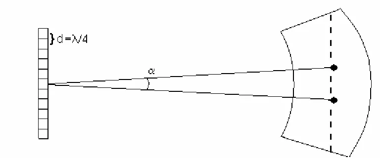
simulations. The sensor arrays are assumed to have an inter-element spacing d equal to

/4, to avoid ambiguity in sensor measurements of a source with wavelength . The size

of the sensor will be discussed in each experiment, since sensors with different amounts

of elements will be simulated. The signals used in each of the experiments will consist of

a pair of point sources that are located at the same range from the center sensor of the

measuring array but separated in angle as shown in Figure 4.1. A field of view is then

measured using the 2D scanning technique mentioned in the Approach, and pictured in

Figure 3.3. The resulting MVDR filter responses for each range and DOA intersection

Figure 4.1- Sensor array angular resolution of a pair of point sources, noted by the angle 

To have accurate resolution in angle and range, the resulting spectral peaks will have a

crest that is located in the correct spatial frequency position of the contour or mesh plot.

If the source pair simulation parameters are manipulated to place the sources closer and

closer, eventually the peaks of each source will start to converge, creating noise and

incorrect spatial frequency peak positions. Minimum angular resolution data was then

taken from the smallest clear angular separation, and care was taken in visually

confirming this data at all values in each experiment in the same manner. In the future, a

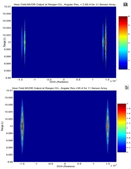
peak identification routine can be written to confirm the resolution as well. To

supplement this discussion, a contour showing acceptable resolution and poor resolution

status can be seen in Figure 4.2. The poor resolution example has multiple noisy spiked

peaks about the actual DOA and range positions of the input simulated source point pair.

Since the DOA and Range positioning of the crest of each peak should correspond to the

The resolution measurements in the following research are gathered using these

inferences. In order to achieve these results, the near field MVDR signal correlation input

is created using ensemble averages of many random initial phase signal records and

periodic time averages, as mentioned in the derivation.

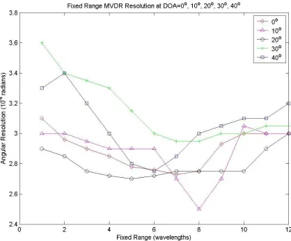
4.2 Experiment 1

The two parameter MVDR algorithm was first tested for imaging resolution of a

source point pair as a function of mean DOA and sensing distance. To measure the

effects of these factors alone, a signal correlation was simulated from 150 noiseless signal

records. The minimum angular resolution was plotted at multiple range distances that

incremented between 1 and 12, to keep within the far field approximation for an 11

sensor array with /4 interelement spacing. The minimum angular resolution between

source point pairs for varying range measurements was then generated for several mean

DOA: broadside (0 for this data), +10, +20, +30, and +40. A plot of resolution

results for each of the signals is posted in Figure 4.2. The angular resolution

measurements have an overall range of 2.5–3.6 10-4 radians, showing no significant

variations. It is valid to say that the angular resolution of this method should be quite

uniform over a wide field of view at any DOA or fixed range. This positive attribute

makes this method much more useful than an imaging technique that suffers from

Figure 4.3 – Source pair resolution at several fixed range distances for a series of DOAs.

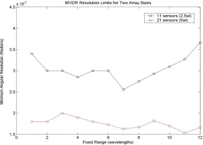
4.3 Experiment 2

This next experiment was conducted with a noiseless signal and 20 signal records

to estimate the improvement in angular resolution by doubling the sensor array length. A

plot in Figure 4.3 provides a resolution comparison of the 11 sensor array with 2.5

indicated that angular resolution is almost 50% better on average for the larger sensor

array. Since a much larger sensor than these is needed for CWD in the near field, it can

be concluded that resolution will not be an issue over these longer ranges.

Figure 4.4 – MVDR method angular resolution as a function of array length, at a broadside DOA

4.4 Experiment 3

To estimate the performance in noise using the same approach as previously

noted, another experiment was simulated. Initial results were attempted by averaging 20

simulated for previous results. Source point pairs located at a mean DOA of broadside

and fixed range of 10 were then resolved at various SNR values. These minimum

angular resolution measurements are plotted for analysis in Figure 4.4.

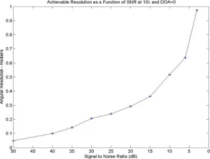
Figure 4.5 – Minimum angular resolution vs. SNR of spectral peaks for 20 averaged records

The y-axis range of the plot in Figure 4.4 corresponds to angular resolution of

2.8 at 50dB and 55.85 at 3dB, which is not particularly reasonable. The resolution plots

revealed a second issue as well, a flattening of the spectral peaks across their range axes.

component of the peak was hard to identify when checking simulation results. This

occurred particularly in plots as the SNR was increased past 40dB, so an increase to 60

records was used to take better source range measurements at 3dB. The range was varied

from 10 to 1 for a few measurements to see if proximity to the sensor array could

increase range resolution. Figure 4.5 is a plot of the pair of spectral peaks identified by

the MVDR filter, and Figure 4.6 shows improvement in range detection for the 1 data.

Figure 4.7 – Angular resolution measurement taken at 1 with 60 records

4.5 Experiment 4

Since the angular resolution and the resolution along the range axis are adversely

affected by both larger range distances and poorer SNR, a better ensemble average is

obviously needed. The objective of experiment 4 was to note the improvements in

resolution as the number of sample records is steadily increased. To do this, the angular

resolution of signals with SNR values of 10dB, 6dB, and 3dB was then obtained as a

Figure 4.8 – Effect of increasing the number of records used in the ensemble average

This plot suggests that using 100 records or more will especially be important to the

sensor data resolution of signals with an SNR value around 3dB. The data taken at 6dB

and 10dB indicate that fewer records are needed to increase the resolution notably, but it

also seems that a noise resolution limit for this small sensor configuration is met at 17.8.

4.6 Experiment 5

For experiment 5, an increase in sensors is seen as another possible method of

resolution enhancement. In addition, a longer aperture length will also allow a much

deeper near field range. Signals were then simulated from an ensemble average of 140

sample records at a SNR value of 10dB, 6dB, and 3dB. The size of the sensor array was

varied using 11 -51 sensors, producing the data set in Figure 4.8.

The information given in Figure 4.8 proves that resolution is significantly enhanced while

the number of sensor elements is increased. This also provides proof that a near field

MVDR method can excel at identification of noisy source distributions and lead to

effective source intensity reconstructions as well.

4.7 Experiment 6

The near field source localization work of Grosicki et al. was reviewed in this

thesis due to its successful use of a desirable Fresnel approximation. The Grosicki et al.

paper also ensured accuracy and prevented phase ambiguities by assuming m  p for a

2p+1 element sensor array, where m is the number of localized sources. To see if the

assumption of Grosicki et al. should also be honored by the MVDR method of the thesis,

an evaluation of this limitation using the two parameter source localization technique is

needed. To test this, equally spaced sources were simulated along a source line in front of

an 11 sensor array with /4 interelement spacing. After some trial and error, seven

sources were simulated over a field of view of 3at positions shown in Figure 4.10.

These sources were then successfully localized as shown in Figure 4.11 using 1000

ensemble average records. The results clearly indicate that this method can resolve more

sources than the approach of Grosicki et al. Please note that the peak at 0 radians only

looks broader than the rest because of the log units used in the plot.

4.8 Near Field Delay and Sum Beamformer Data

To gauge the usefulness of the previous data taken by the Near-Field MVDR

method, a simpler method was attempted in a data comparison effort. A simpledelay and

sum beamforming method was implemented to provide this comparison. A traditional

delay and sum beamformer identifies the source DOA of far field signals by totaling the

signals from each sensor when the signal is delayed by a certain phase:

 

X

p

p k input Sum

Delay    

      



 exp 2 sin (4.1)

Delay and sum (4.1) does not use the correlation matrix like a MVDR filter, but produces

peaks when the phase product between the signal and steering vector produces a

maximum. If d is measured in wavelength units, we can assume =1 in (4.1). The only

drawback to the function is that excessive oversampling is needed to get a precise

response in many far field cases. To reconfigure delay and sum for near field sources and

index the sensors as –p ≤ k≤ p, the following expression involving range and DOA may

be used:

 













2 exp

,_{r x j r}2 _k2_d2 _kd X p p k input Sum Delay (4.2)

The square root in (4.2) is a geometrically derived expression for the diagonal distance

from the source to each k-indexed sensor. Several results were then derived with this

equation without noise using similar array sizes, ranges, and DOA measurements to the

Table 4.1 – Resolution Comparison of ‘Delay and Sum’ and Near Field MDVR Method

Range from 11 Element

Sensor Array Delay and Sum Resolution(radians) MVDR Resolution(radians)

1 0.795 0.00031

1.5 1.10 0.0003

Range from 21 Element Sensor Array

Delay and Sum Resolution (radians)

MVDR Resolution (radians)

1 0.622 0.00018

2 0.827 (DOA = 0)

0.873 (DOA = 30) 0.00018

3 1.14 (DOA = 0) 0.0002

The spatial frequency peaks of the Delay and Sum method for 11 and 21 sensors that

were generated within a 1 range were distinct but had large sidelobes. As the Delay and

Sum measurements of both sensor arrays were attempted at slightly larger ranges, the pair

of peaks increase in width at an exponential rate. As a result, increases in range beyond

1.5 for the 11 sensor array, and 3 for the 21 sensor array, lead to inconclusive Delay

and Sum measurements. An example of the near field delay and sum plots used in these

calculations is in Figure 4.12. The results posted in Table 4.1 and this discussion show

that accuracy and resolution are faulty in this implementation of the Delay and Sum

method, and that the range limitations are an issue as well. This also establishes why

there is a credible need for precise peak results from a method like the Near-Field MVDR

Chapter 5

Conclusion

Through the course of this research, a new algorithm was developed to perform

high resolution spectral analysis of source points in the near field. The need for effective

field measurement algorithms in high frequency concealed weapon detection has been

established. Several previous methods and procedures have been outlined, along with

their groundbreaking results and restrictions. This thesis then outlined a desired 2D

localization method based on a MVDR routine that calculates filter responses along range

and DOA axes. This method was tested with signals of varying noise and direction, but

continued to show promise in simulations. Simulations were able to predict limitations to

resolution as a result of sensor size and distance from the array. Sources that are close to

the array were much easier to resolve along the range axis than those placed towards the

far field threshold. Direction of arrival resolution was maximized by both increasing the

record samples used to calculate the ensemble average, and increasing the number of

sensor elements to enhance sensitivity. Some of the background literature that has been

analyzed in this thesis has shown that there are still more ways of increasing the

efficiency and sensitivity of methods such as this.

In future studies, one of the first directions for research with a MVDR algorithm

would be testing with actual data. If output from a uniform linear array of known size is

could be attempted with lines of horizontal data initially, and then modified into a two

dimensional method. In two dimensions, the algorithm would need to allow measurement

of sources by horizontal DOA, vertical pitch angle, and by their approximate range. In

order for this to be possible, a method must be coupled with the MVDR filter output to

correctly identify the intensities of the localized field sources. This could be achieved by

such means as an eigenspace solution, least squares routine, or a set of optimization

commands. Another challenge that may be presented in actual data is obtaining desired

results despite hardware limitations, since high frequency sources have brief periods.

A second direction for accomplishment in an MVDR method would be to apply it

to wideband data. There are several current methods for wideband data analysis, and

research such as that presented by J. C. Chen et al. provides a catalyst for weapon

detection using wideband localization of high frequency sources (J. C. Chen et al., 2002).

Wideband methods have already shown resolution improvements in their

millimeter-wave scanning portal technology as well (Sheen et al., 2001). Since certain terahertz

frequencies would aid detector units in automatic identification of concealed explosive

Appendix 1

Table of Abbreviations

CWD Concealed Weapon Detection

dB Decibels

DOA Direction of Arrival

GHz Gigahertz

MUSIC Multiple Signal Classification

MVDR Minimum Variance Distortionless Response

PSD Power Spectral Density, also referred to as the ‘Spectrum’ of a signal

RMSE Root Mean Square Error

SNR Signal to Noise Ratio

THz Terahertz

THz-TDS Terahertz Time-Domain Spectroscopy

Appendix 2

MATLAB Source Code for Correlative Interferometry

function thzImage(xv,ex,yv,snr)

% Written by Joseph Handfield ~ongoing revisions 6/12/06 %

% This function calculates an array of spatial correlations of the sensed field % using an appended array (first half of columns are real parts, others are % imaginary). It also calculates a theoretical correlation using the

% solution to its integral. The output is an intensity array indicating the % location of the sources from the least squares computation of both % correlations.

%

% thzImage uses inputs:

% yv = Array of sensor locations along the sensing line, less than