City, University of London Institutional Repository
Citation
:
Reyes-Aldasoro, C. C., Björndahl, M. A., Akerman, S., Ibrahim, J., Griffiths, M. K. and Tozer, G. M. (2012). Online chromatic and scale-space microvessel-tracing analysis for transmitted light optical images. Microvascular Research, 84(3), pp. 330-339. doi: 10.1016/j.mvr.2012.09.002This is the unspecified version of the paper.
This version of the publication may differ from the final published
version.
Permanent repository link:
http://openaccess.city.ac.uk/3736/Link to published version
:
http://dx.doi.org/10.1016/j.mvr.2012.09.002Copyright and reuse:
City Research Online aims to make research
outputs of City, University of London available to a wider audience.
Copyright and Moral Rights remain with the author(s) and/or copyright
holders. URLs from City Research Online may be freely distributed and
linked to.
Title:
Online chromatic and scale-space microvessel-tracing analysis for transmitted light optical images
Authors:
Constantino Carlos Reyes-Aldasoro1,2*, Meit A. Björndahl2,3, Simon Akerman2,4, Jamila Ibrahim2 , Michael K. Griffiths5 andGillian M. Tozer2
1 Biomedical Engineering Research Group, Department of Engineering and Design, 2B10 Shawcross Building, University of Sussex, Falmer, Brighton, BN1 9QT, UK.
2 Tumour Microcirculation Group, CR-UK/YCR Sheffield Cancer Research Centre, Department of Oncology, The University of Sheffield, F Floor, School of Medicine, Beech Hill Road, Sheffield S10 2RX, UK
3 Current address: SentoClone International AB, Norrmalmstorg 14, 111 46 Stockholm, Sweden
4 Current address: Department of Neurology, UCSF School of Medicine, 513 Parnasus Avenue, San Francisco CA 94143, USA.
5 Corporate Information and Computing Services, The University of Sheffield, 285 Glossop Rd. Sheffield, S10 2HB, U.K.
* Corresponding author: Email: [email protected]
Abstract
Limited contrast in transmitted light optical images from intravital microscopy is problematic for analysing tumour vascular morphology. Moreover, in some cases, changes in vasculature are visible to a human observer but are not easy to quantify. In this paper two online algorithms are presented: scale- space vessel tracing and chromatic decomposition for analysis of the vasculature of SW1222 human colorectal carcinoma xenografts growing in dorsal skin-fold “window” chambers in mice. Transmitted light optical images of tumours were obtained from mice treated with the tumour vascular disrupting agent, combretastatin-A-4-phosphate (CA4P), or saline. The tracing algorithm was validated against hand-traced vessels with accurate results. The measurements extracted with the algorithms confirmed the known effects of CA4P on tumour vascular topology. Furthermore, changes in the chromaticity suggest a deoxygenation of the blood with a recovery to initial levels in CA4P-treated tumours relative to the controls. The algorithms can be freely applied to other studies through the CAIMAN website (CAncer IMage ANalysis: http://www.caiman.org.uk).
Keywords
Introduction
Analysis of microvascular images from intravital microscopy is important in a number of biomedical applications (Bagher et al., 2011; Gavins and
Chatterjee, 2004; Hughes and Gavins, 2010; Koschwanez et al., 2010; Tabuchi et al., 2008). In cancer, intravital microscopy has become an important tool to analyse angiogenesis (Fukumura et al., 2010; Vajkoczy et al., 2000), metastasis (Beerling et al., 2011), red blood cell velocity (Reyes-Aldasoro et al., 2008), blood supply (Brurberg et al., 2008; Tozer et al., 2005a), lymphatic observation (Gaustad et al., 2012) amongst other processes (Lunt et al., 2010; Zomer et al., 2011).The established tumour vasculature is also considered an important therapeutic target (Dumontet and Jordan, 2010; Ma and Adjei, 2009; Tozer et al., 2005b). Intravital microscopy is particularly useful for longitudinal studies, as it is possible to visualise the changes of the vasculature: growth, reversion, haemorrhage, etc. over several days. Fluorophores are commonly used with intravital microscopy (Lunt et al., 2010; Masters, 2010) to provide a target structure with high visual
discrimination. However, despite its usefulness, fluorescence intravital microscopy has limitations such as photobleaching and phototoxicity, such that transmitted light optical imaging is preferred in some cases.
While a visual observation of the vasculature can reveal important
characteristics, in understanding the growth of the vasculature and the action of vasoactive drugs, a quantification of vascular structures and its variation is crucial. The vasculature can be quantified through its topology (number, size, distribution of the vessels, etc.) or its function. Changes in chromatic
characteristics of images containing blood vessels relate to vascular function via the dependence of the absorbance spectra of haemoglobin on oxygen saturation. In this work, we concentrate on two quantifiable aspects of microvasculature as observed through optical intravital microscopy: colour and topology.
Colour in a digital image is described by the combination of three or four values of single primary or derived colours, these combinations are called colour spaces or models. Perhaps the most widely used colour space is the one formed by red, green and blue channels (RGB). However, there are many other colour spaces, such as the YUV (luminance and chrominance) used for analogue colour television or CMYK (cyan, magenta yellow, black) used in printing. A common space used for biomedical image analysis is the Hue, Saturation and Value (HSV) (Maximova et al., 2006; Reyes-Aldasoro et al., 2011b; van Der Laak et al., 2000). The HSV space describes perceptual colour relationships related to the artistic ideas of hue, tint and shade (Gonzalez and Woods, 2008; Smith, 1978), which provide a more natural description of colour than additive or subtractive colour components.
L-Lightness, B-Brightness) arise. The advantage of these spaces is that the hue has been decoupled from the purity (saturation) and the intensity or darkness, which are all combined when the RGB primary colours are used. Quantification of the chromatic characteristics of an image can be performed on the numerical values of the channels, or on measures derived from them, such as histograms, which have been used in one (Schettini, 1993), two (Angulo and Serra, 2005; Angulo and Serra, 2007; Hanbury and Serra, 2003) and three dimensions (Cho et al., 2001; Reyes-Aldasoro et al., 2011b) in different biomedical applications.
To analyse the topological variations of the vasculature it is necessary first to obtain a mathematical description of one or more parameters of the vessels like vessel diameter or length. These parameters can be measured directly, for instance vessel diameters from murine dorsal skin-fold chambers (Morris and Skalak, 2007), or indirectly from a more complex description, like tracing of meningial blood vessels in exposed cranial matter (Fischer et al., 2010). It is common to obtain the parameters through manual measurements or delineation (as in the previous two examples). These manual procedures are time consuming and subjective, however, they are still widely used and form the gold standard for testing automatic algorithms.
Several semi-automatic algorithms have been developed to obtain topological parameters. Barber (Barber et al., 2003) developed semi-automatic software to trace fluorescent vessels from intravital images of tumours, where a user selects points of a 3D intensity dataset to generate traces. A model-based training algorithm where a geometric model identifies bifurcation of vessels was proposed in (Delibasis et al., 2010). This model produced good results for retinal images, but required training and testing data sets, which are not
always available. Fischer (Fischer et al., 2010) proposed a semi-automated methodology to measure meningeal blood vessel diameter as observed through cranial windows with light microscopy. The algorithm was released as an ImageJ (National Institute of Health, USA) plug-in, and required to have a reference image and a posterior image in time to perform digital subtraction as well as a manually-traced profile from which the diameter was measured. Abdul-Karim (Abdul-Karim et al., 2003) proposed an automatic tracing
algorithm for 3D datasets from murine mammary adenocarcinoma growing on SCID mice acquired with multiphoton microscopy. This algorithm required a difference of intensities between the vessels and the background, which is not always possible in the case of light microscopy. Another robust algorithm that required that the background intensity levels drop to minimum levels with respect to the vessel intensities was proposed by Tyrrell (Tyrrell et al., 2007; Tyrrell et al., 2005). In this study, the vessels of carcinomas observed with dorsal skin-fold chambers were modelled by fitting a super-Gaussian function to create a superellipsoid that followed the drop in intensity. The fitting
For the current work we implemented two automatic algorithms, with online access, to obtain quantitative measurements related to the chromaticity and vascular tracing of tumour microvessels. The algorithms were developed in
MATLAB (© MathWorks, USA), implemented on a high-performance cluster, and are made available through a website (http://www.caiman.org.uk). A 3D chromatic histogram describing the chromatic characteristics of an image was developed previously for analysis of histological tissue sections (Reyes-Aldasoro et al., 2011b) and is implemented here for intravital imaging of tumours. We also implemented a scale-space ridge detection algorithm (Lindeberg, 1998a; Lindeberg, 1998b) as a fully automatic vessel tracing algorithm. The scale-space algorithm is a multiscale technique in which a progressive filtering or smoothing is applied to an image with the intention of detecting features (ridges, edges, blobs, etc.) of different dimensions at different scales. Therefore, sharp features will be detected at fine scales, that is, those that have been slightly smoothed, whilst coarse features will be detected with considerable smoothing of the images. Both algorithms are “intensity-based” as opposed to clustering or deformable models (see (Ma et al., 2010) for a review of Medical Image Segmentation techniques), and the scale-space algorithm belongs to the “Ridge detection - Pattern Recognition” techniques (see (Kirbas and Quek, 2004) for a review of Vessel Extraction Techniques).
The algorithms were tested on the microvasculature of SW1222 human colorectal carcinoma xenografts growing within surgically implanted dorsal skin-fold ‘window’ chambers in mice, in order to determine whether they could detect the well-known tumour vascular modifying effects of the vascular disrupting agent (VDA), combretastatin-A-4 3-0-phosphate (CA4P) (Tozer et al., 2005b).
(D)
Longitudinal studies of chromaticity (hue, saturation and value) and vessel characteristics (average vessel length, average vessel diameter, vessel density) were performed with the algorithms over a period of 24 hours after a single dose of CA4P or a saline equivalent.Material and methods
All animal experiments were conducted in accordance with the United Kingdom Home Office Animals (Scientific Procedures) Act 1986, with local ethical approval and in line with recently published Guidelines for the Welfare of Animals in Cancer Research (Workman et al., 2010). Surgical procedures were as described previously (Tozer et al., 2005a). Briefly, an aluminium window chamber (total weight 2g), designed to hold two parallel glass
Hanging drops were established from 1x10⁵ SW1222 cells in 20 µl DMEM supplemented with 10% FCS and 4 mmol/L glutamine plus standard
antibiotics. After 3-4 days of growth, the cell aggregates from the drops were transplanted directly onto the exposed panniculus muscle within the dorsal skin-fold window chamber preparations and the chambers closed with a glass cover-slip.
After approximately 10-12 days, when tumour growth was established, transmitted light images of the tumours were acquired using a Nikon Eclipse E600FN microscope incorporating illumination from a 12V/100W halogen light source.
(B2)
Ninety six transmitted light images (x10 objective) were acquired from 6 restrained window chamber-bearing mice: CA4P-treated (n=3) or control (saline-treated, n=3) in 2 regions of interest (centre and periphery of tumour) before (time=0) and up to 24h (2.5, 15, 30, 60, 180, 360, 1440 min) after treatment with 30 mg/kg of CA4P or saline administered intraperitoneally (i.p.). CA4P was kindly supplied by Professor GR Pettit, Arizona State University, Tempe, AZ, USA. The images were uploaded to CAIMAN where they were processed with the algorithms described below.
(A)
Algorithms
The chromaticity algorithm considered that a colour image in the RGB colour space, Irgb has dimensions Nr Nc 3 for rows, columns and three colour
channels [R,G,B]red, green and blue. Hue, h, h[0,360°), is a circular property related to the wavelength of the colour where red corresponded approximately to 0°, yellow to 60°, green to 120°, cyan to 180°, blue to 240° and magenta to 315°. The saturation s, s[0,1], is a measure of the purity of the colour or its departure from white or grey and value v, v[0,1], is a measure of the brightness.
The hue-saturation-value histogram is a tri-variate measurement of the relative frequency of [H,S,V] on Ihsv and it was defined (Reyes-Aldasoro et al.,
2011b) as:
,
where # denoted the number of elements in the set. Besides the 3D histogram mHSV (h,s,v), some of its marginal distributions are also useful.
A marginal distribution of a n-dimensional distribution corresponds to the distribution when one of the dimensions is averaged over the other
interest for that marginal (Leon-Garcia, 1994). The marginal distribution of mHSV (h,s,v) along the value dimension corresponds to the 2D hue-saturation
histogram , which is a useful tool to explore and segment chromatic images. One-dimensional marginal distributions are obtained with a double summation, for instance: .
(C1)
Fig. 1a-c shows one representative image with its corresponding 2D and 3D histograms. The 2D histogram is shown as a black mesh where height corresponds to occurrence of pixels with the pair of hue-saturation described by the loci of constant value that is displayed under the mesh. The 3D
histogram is described by a cloud of points located at the corresponding chromatic location and whose size corresponds to the occurrence of the pixels with the triplet hue-saturation-value and the colour. The centroid of the mHSV (h,s,v) cloud (cHSV (h,s,v) is used as a numerical descriptor to summarise
the chromatic characteristics of an image, as small colour variations can be recorded by the position of the centroid.
To estimate the centroid of the 3D cloud, the weighted average of the vector that described each of the dimensions (h=[0,…,360°), s=[0,…,1], v=[0,…,1]) and the individual 1D marginal distributions (mH (h), mS (s), mV (v)) were
obtained. For s and v the calculation is direct:
,
where sn, vn correspond to the quantised values of each vector.
However, to calculate cH there is an extra consideration as hue is a circular
property; for instance, 350° is equivalent to -10°. To calculate the correct centroid, the vector h=[0, … 360°) was circularly rotated to align the region [0, … 180°) with the bulk of the cloud. Then, the weighted average that
corresponded to the rotated centroid was calculated and the inverse rotation was applied to obtain the correct centroid. The three values cH, cS, cV are
directly provided by the algorithm.
(C2)
The vessel tracing algorithm used a scale-space approach (Lindeberg, 1998b), which analysed the differences in intensity of neighbouring pixels. The centreline of vessels was detected as a “ridge” in a topographical analogy and successive levels of filtering or blurring provided different scales to detect sharp to diffuse ridges. Details of the scale-space algorithm can be found in (Lindeberg, 1998a), but briefly, scale-space representation of a function f(x,y) can be defined as the convolution with a Gaussian g(x,y;t) where t
L(x,y;t)g(x,y;t) f(x,y) 1 2t
e(x2y2) / ( 2t)
f(x,y).
Then, the normalised first and second derivatives in x and y dimensions (Lx,
Lxx, Ly, Lyy), which form the Hessian Matrix:
H
xxf yxf
xyf yyf
Lxx Lyx Lxy Lyy
,
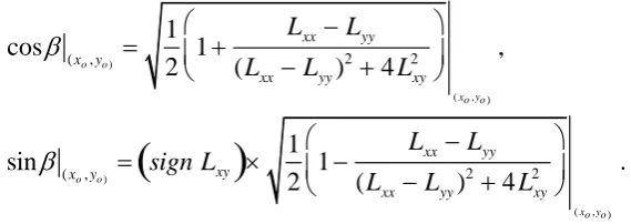
highlighted the rate of change of the intensities of the images. Regions of maxima and minima were calculated when the derivatives reached zero. To obtain the centrelines of vessels, or ridges in a topological analogy, it was necessary to convert from the (x,y) coordinate system to a local (p,q) system aligned with the eigendirections of H:
Lp pL(sin x cos y)L,
Lq qL(cos x siny)L,
Lpq pqL(cosxsin y)(sinxcosy)L,
where
denotes the angle of rotation of the coordinate system and it was defined by:
cos(x
o,yo)
1 2 1
Lxx Lyy
(Lxx Lyy)
2
4Lxy 2
(xo,yo)
,
sin(x
o,yo)
sign Lxy
1 2 1
Lxx Lyy
(Lxx Lyy)2
4L2xy
(xo,yo)
.
The ridges at different scales constituted a scale-space ridge surface and were defined as the points of (Lp, Lpp, Lq, Lqq) that fulfilled the conditions of
[image:8.595.88.373.434.535.2]maxima at every scale. Finally, a scale-space ridge was simplified from the ridge surface by selecting the points where the surface had maximal values by a given norm. Thus, fine ridges were detected at fine scales whilst coarse ridges had higher norm values at larger scales. The detected scale-space ridges were ranked by the saliency of the ridge, which indicates which ridges are better defined in the contrast between the ridge itself and the surrounding regions. The scale-space ridges defined the outlines of the visible vasculature within each image, from which the algorithm calculated several descriptive measurements detailed below.
black. In 1f, some ridges are displayed in 3D with the scale, which is related to the diameter, as the z-axis.
(C3)
Both algorithms were implemented on the CAIMAN website
(http://www.caiman.org.uk) (Reyes-Aldasoro et al., 2011a), which is publically accessible for other researchers to use. The 96 images in the current study were uploaded to the web-server. From here, the system works by
transferring them to a high performance cluster for processing in MATLAB.
The results are then sent back via email
(A)
. A screen shot of the CAIMAN webpage for the tracing algorithm and an example email sent by CAIMAN are shown in Fig. 2.(C4)
For the chromatic analysis, the email contains the centroids, the ratios of the
HSV channels, which indicate the distribution of colour in the channels, and one MATLAB file with a 32x32x32 matrix, which corresponds to the mHSV
histogram, where the three dimensions are quantised to 32 levels. From this matrix, the centroid of the cloud of points in the histogram was calculated for each dimension as described above.
For the vessel tracing algorithm, the email contains two attachments: an image file with the tracing overlaid on the original image (Fig. 1e) and a
MATLAB file with the ridges as 3D matrix where the rows and columns correspond to the position of the vessels in the image and the levels or third dimension to the scale at which the ridge was detected. This level is
proportional to the diameter of the vessel itself. The ridges are labelled, i.e. first ridge is denoted by ones in the matrix, the second by twos and so on. The lines of Fig. 1e,f were generated from this matrix. From this second file, a user could extract more measurements, such as tortuosity of the ridges, if required. Together with the attachments the following measurements are provided in the email: number of vessels or ridges that were detected by the algorithm,
total length, average vessel length, average vessel diameter. In addition, these last 3 measurements are also provided for the 10 ridges with the highest saliency, i.e. the most important ones according to the algorithm (labelled in red in Fig. 1e). The average vessel length measurements are calculated from the distance covered by each ridge, noting that a vessel is defined here as each individual ridge that is detected by the algorithm. The ridge is defined by the changes in intensity and/or a branch point in the vascular network. Thus, a physical vessel between two branch points may be composed of more than one ridge, if there is a decrease of intensity along the length of its centreline. At a branch point, the ridge may continue along one branch, in which case a second ridge is created along the other branch; or, if there is a sudden change of intensity at the branch point, 3 ridges may be formed. The same situation may occur where vessels cross at different depths within the tissue. Since a 'vessel', as defined above, describes various
Fig. 1f), coarse for wider vessels (high in Fig. 1f). The vascular density is calculated as the number of traced vessels per tumour area per given image. The total vascular length is calculated as the sum of the lengths of all
individual ridges per tumour area per given image. All measurements are calculated in pixels, which can later be calibrated to m depending of the magnification of the microscope, if so required.
(J)
The vessel-tracing algorithm was validated manually with a custom-made
MATLAB graphical user interface. All data sets at time t=0 [s] (n=12) were hand-traced in a process blind to the automatic tracing. The accuracy of the manual tracing versus the automatic was estimated through a measurement of the distance between the manual and automatic traces. Starting from the vessels of each case, the minimum distance from each pixel in the image to the closest vessel was calculated, this is called a distance map. Next, the hand-traced vessels were overlaid on the automatic distance map and vice versa to measure the distance from one set to the other. The distances were then measured in cumulative histograms. The process is illustrated in Fig 3.
The sensitivity of the vessel tracing algorithm to the quality of the image was tested by degrading the image and measuring the distance from the automatic traces of the degraded image against the hand-traced vessels. The images were degraded in two ways: (a) adding white Gaussian noise and (b) blurring the image with a low pass filter.
(C6)
Results and Discussion
The 96 images described in Materials were processed through CAIMAN: the images were uploaded through the website, processed in the High
Performance Cluster and results returned by email, from where the measurements were collected to perform the statistical analysis.
(A)
The results of vessel tracing are illustrated for a single image in Fig. 1e,f. The algorithm detected 355 ridges with average lengths and diameters of 31.9 and 10.1 pixels respectively. The corresponding measurements for the 10 most salient ridges (Fig. 1e, red lines) were 127.6 and 15.1, which indicated that the most salient ridges were considerably longer and wider than the rest (green and black lines). The 50 most salient ridges (red and green in Fig 1e) concentrated on the right side of the image where the vasculature was well defined, but ridges were also detected in the left side. The scale of detection is illustrated in Fig. 1f where the z-axis corresponds to the scale; the height is proportional to the diameter of the vessels as it can be seen from the two long red lines in the centre of the image. For clarity only some of the black lines were plotted.
The automatic algorithm traced a larger number of vessels than the manual user, mainly thin, faint vessels that were hard to distinguish visually.
Therefore, the distance from the manual vessels to the automatic vessels was considerably smaller than the opposite case. This was reflected on the
histograms; in Fig. 4a 90% of all manual traces were located within a distance of 12 pixels from the automated traces, whilst in Fig. 4b 90% of all automated traces were located within a distance of 20 pixels from the manually traced vessels. It should be noted that traces produced by the two methods for a single vessel, whilst both correct, could still be a few pixels away from each other. The average vessel diameter from the 96 images, measured by the automatic algorithm, was 13.6 pixels. Therefore, discrepancies between the two methods below this value correspond to traces that are very close to each other and, in most cases, represent the same blood vessel.
The chromatic analysis algorithm produced mHSV from which the centroid of
the cloud of points was obtained for H, S, and V. Fig. 5 shows the time course of the tumour images and their corresponding 3D histograms for one case treated with CA4P and one control. It should be noted how the cloud shifts in
H (a small cloud appears on the left side at 15 min) as well as in S and V
(cloud moves "forward" and down) for the treated case. At 3h there is a
change in colour noticeable by the disappearance of the cloud on the left. The control remains in the same range of H,S,V throughout the time course of the observation.
(E)
The temporal effects of the vascular disrupting agent CA4P were analysed for the full 96-image data-set for 6 measurements: hue, saturation, value (Fig. 6),
average diameter, average length, vessel density and total length per area
(Fig. 7). In both figures, the top row shows the absolute values and in the bottom row the lines have been normalised relative to the initial time point.
(A)
Thin blue lines with round markers correspond to CA4P treated tumours, while thin red lines with square markers correspond to saline, the thick lines correspond to the averages of each group at every time point. It is important to notice that the two methods are independent of each other, that is, the extraction of chromatic characteristics do not have any relationship with the tracing algorithm.
presented a slight decrease of V (that is, became darker) and recovered between 1 and 3h, while the saline group showed the opposite trend. While the average length and total length per area of the vessels remained constant after treatment with a saline solution, these parameters decreased by approximately 13% up to 1h after CA4P treatment with a subsequent recovery (Fig. 7a,d,e,h). This is consistent with previous results in a rat tumour model, where vessel segments were manually quantified and is
indicative of loss of red cells, either because of upstream vascular constriction or vascular collapse, rather than permanent vascular destruction (Tozer et al., 2001).
(G)
The vessel diameter of the CA4P-treated group also showed a reduction with a minimum at 1h, whilst the vessel diameter in the saline-treated group remained constant (Fig. 7b,f). The vessel density remained relatively constant for both groups (Fig. 7c,g). The decrease in averagelength, average diameter and total length density of vessels between 0 and 1h for the CA4P group results in a smaller area of the tissue being covered by vessels, even when the vessel density remained constant. This is consistent with the decrease in saturation observed at this time-point. Between 1h and 3h the vessels became longer and wider in the CA4P group, returning towards baseline values, suggesting recovery from the effects of the drug. However, at 3h, the hue is well below baseline (deep red to purple)
suggesting an additional effect, namely de-oxygenation of haemoglobin. This is consistent with severely compromised tumour blood flow, even when the visible vasculature has returned to normal, as reported for CA4P previously (El-Emir et al., 2005; Murata et al., 2001; Prise et al., 2002; Wang et al., 2009).
(F,H,K)
The current results show that recovery in the length and diameter of the
measured microvessels towards baseline by 3h is not sufficient to re-establish baseline oxygenation. A continued blood flow shut-down and de-oxygenation of haemoglobin under these conditions is most likely due to continued
resistance to flow either due to haematological disturbances such as red cell stacking and/or coagulation or continued constriction of down-stream draining vessels (Busk et al., 2011; Prise et al., 2002; Tozer et al., 2001)
It is important to mention that while the results of the tracing algorithm are relatively immune to variations of the acquisition, i.e. illumination, the chromatic characteristics may change with different conditions. We have attempted to minimise these effects by analysing only the hue and the saturation, as changes in brightness such as those created by changing illumination in a microscope, should be reflected mainly in the value, i.e. the clouds of Figs. 1c, 4 moving up and down but not sideways. Still, as in any other experiments, it is desirable to keep conditions constant throughout the acquisition of the data.
noise, the better tracing it will produce. Fig. 8a shows one representative image and 8b shows the effects of the degradation process described in Materials and Methods. The effects of the added noise at 5 increasing intensity levels are shown on the upper half of the image, where it can be seen how the image is more “grainy” towards the right hand side. The increasing blur produced by filtering are shown on the bottom half of the image from less blurred on the left and more blurred on the right. Fig 8c shows the effects of image degradation on the distance between manual and automatic traces. The distance between the automatic traces produced by the algorithm and the manual delineation of the vessels increased monotonically as the level of white Gaussian noise increased (solid line with diamond marker), as it would be expected as the noise diverted the ridges from it correct position. When the blurring was introduced, a small blur reduced the distance suggesting that the original image contained a small amount of noise, which when removed by the filtering, reduced the distance between traces (dotted line with circular markers). However, as the blurring increased, the error distance increased monotonically as the blurring must have removed small thin vessels and diverted the ridges from its original position.
(L)
A future development of the current work would be to combine the two algorithms to provide a chromatic description of the blood vessels, independently of the surrounding tissue. This would allow a more direct analysis of haemoglobin oxygen saturation.
(I)
Conclusion
In this work we presented two methodologies for the study of microvasculature observed from optical light images. The scale-space tracing algorithm detected the vasculature of in vivo light microscopy images successfully, whilst the chromatic analysis allowed the tracking of the centroids of 3D histograms with time. The tracing algorithm successfully monitored the well known effects of CA4P treatment on the topology of tumour blood vessels i.e. it reduced the average diameter and length of vessels for a limited time (Tozer et al., 2008; Tozer et al., 2001) whilst the chromatic analysis provided additional functional information.
(D)
The online interface allowed the submission of images without the need for users to do any programming or installation of any software.Acknowledgements
We thank Prof Barbara Pedley from University College London for supplying the cells and Prof Bob Pettit from Arizona State University for supplying the CA4P used in this study. We thank staff at The University of Sheffield for their care of the animals. We thank the White Rose Grid and The University of Sheffield for “iceberg”, the computing facilities to run the Caiman website and Dr. Deniz Savas from Corporate Information and Computer Services for his support.
Abdul-Karim, M. A., et al., 2003. Automated tracing and change analysis of angiogenic vasculature from in vivo multiphoton confocal image time series. Microvasc Res. 66, 113-25.
Angulo, J., 2006. Morphological color image simplification by saturation-controlled regional levelings. International Journal of Pattern Recognition and Artificial Intelligence. 20, 1207-1223.
Angulo, J., Serra, J., 2005. Image Color Segmentation using Bi-variate Histograms in Luminance/Saturation/Hue Polar Color Spaces. Computac. Sist. 8, 303-316. Angulo, J., Serra, J., 2007. Modelling and segmentation of colour images in polar
representations. Image and Vision Comput. 25, 475-495.
Bagher, P., et al., 2011. Intravital macrozoom imaging and automated analysis of endothelial cell calcium signals coincident with arteriolar dilation in Cx40(BAC) -GCaMP2 transgenic mice. Microcirculation. 18, 331-8.
Barber, P. R., et al., 2003. Semi-automated software for the three-dimensional delineation of complex vascular networks. J Microsc. 211, 54-62.
Beerling, E., et al., 2011. Intravital microscopy: new insights into metastasis of tumors. J Cell Sci. 124, 299-310.
Brurberg, K. G., et al., 2008. Temporal heterogeneity in blood supply in human tumor xenografts. Neoplasia. 10, 727-35.
Busk, M., et al., 2011. Combretastatin-induced hypertension and the consequences for its combination with other therapies. Vascular Pharmacology. 54, 13-7.
Cho, K. M., et al., 2001. Adaptive skin-color filter. Pattern Recognit. 34, 1067-1073. Delibasis, K. K., et al., 2010. Automatic model-based tracing algorithm for vessel
segmentation and diameter estimation. Computer Methods and Programs in Biomedicine. 100, 108-122.
Dumontet, C., Jordan, M. A., 2010. Microtubule-binding agents: a dynamic field of cancer therapeutics. Nature Reviews Drug Discovery. 9, 790-803.
El-Emir, E., et al., 2005. Tumour parameters affected by combretastatin A-4 phosphate therapy in a human colorectal xenograft model in nude mice. Eur J Cancer. 41, 799-806.
Fischer, M. J. M., et al., 2010. Measurement of meningeal blood vessel diameter in vivo with a plug-in for ImageJ. Microvascular Research. 80, 258-266.
Fukumura, D., et al., 2010. Tumor microvasculature and microenvironment: novel insights through intravital imaging in pre-clinical models. Microcirculation. 17, 206-25.
Gaustad, J. V., et al., 2012. A novel application of dorsal window chambers: Repetitive imaging of tumor-associated lymphatics. Microvascular Research. 83, 360-5.
Gavins, F. N., Chatterjee, B. E., 2004. Intravital microscopy for the study of mouse microcirculation in anti-inflammatory drug research: focus on the mesentery and cremaster preparations. J Pharmacol Toxicol Methods. 49, 1-14.
Gonzalez, R. C., Woods, R. E., 2008. Digital image processing. Pearson Prentice Hall, Upper Saddle River, NJ.
Hughes, E. L., Gavins, F. N., 2010. Troubleshooting methods: Using intravital microscopy in drug research. J Pharmacol Toxicol Methods. 61, 102-12.
Kirbas, C., Quek, F., 2004. A review of vessel extraction techniques and algorithms. Acm Computing Surveys. 36, 81-121.
Koschwanez, H. E., et al., 2010. Intravital microscopy evaluation of angiogenesis and its effects on glucose sensor performance. J Biomed Mater Res A. 93, 1348-57.
Leon-Garcia, L., 1994. Probability and Random Processes for Electrical Engineering. Addison-Wesley Publishing, Reading, Mass.
Lindeberg, T., 1998a. Edge detection and ridge detection with automatic scale selection. Int J Comp Vision. 30, 117-154.
Lindeberg, T., 1998b. Feature detection with automatic scale selection. Int J Comp Vision. 30, 79-116.
Lunt, S. J., et al., 2010. The Application of Intravital Microscopy in Studies of Tumour Microcirculation. J Biomed Optics. 15, 11113.
Ma, W. W., Adjei, A. A., 2009. Novel Agents on the Horizon for Cancer Therapy. Ca-a Cancer Journal for Clinicians. 59, 111-137.
Ma, Z., et al., 2010. A review of algorithms for medical image segmentation and their applications to the female pelvic cavity. Comput. Meth. Biomech. Biomed. Eng. 13, 235-246.
Masters, B. R., The Development of Fluorescence Microscopy. Encyclopedia of Life Sciences. John Wiley & Sons, Chichester, 2010.
Maximova, O. A., et al., 2006. Computerized morphometric analysis of pathological prion protein deposition in scrapie-infected hamster brain. J. Histochem. Cytochem. 54, 97-107.
Morris, C. E., Skalak, T. C., 2007. Chronic static magnetic field exposure alters microvessel enlargement resulting from surgical intervention. Journal of Applied Physiology. 103, 629-636.
Murata, R., et al., 2001. Comparative effects of combretastatin A-4 disodium phosphate and 5,6-dimethylxanthenone-4-acetic acid on blood perfusion in a murine tumour and normal tissues. Int J Radiat Biol. 77, 195-204.
Prise, V. E., et al., 2002. The vascular response of tumor and normal tissues in the rat to the vascular targeting agent, combretastatin A-4-phosphate, at clinically relevant doses. Int J Oncol. 21, 717-726.
Reyes-Aldasoro, C. C., et al., 2008. Measuring the velocity of fluorescently labelled red blood cells with a keyhole tracking algorithm. J Microsc. 229, 162-173. Reyes-Aldasoro, C. C., et al., 2011a. CAIMAN: An online algorithm repository for
Cancer Image Analysis. Comput. Meth. Prog. Bio. 103, 97-103.
Reyes-Aldasoro, C. C., et al., 2011b. An automatic segmentation algorithm for the morphological analysis of microvessels in immunostained histological tumour sections. J Microsc. 242, 262-278.
Schettini, R., 1993. A segmentation algorithm for color images. Pattern Recognit. Lett. 14, 499-506.
Smith, A. R., 1978. Color gamut transform pairs. ACM Siggraph Computer Graphics. 12, 12-19.
Tabuchi, A., et al., 2008. Intravital microscopy of the murine pulmonary microcirculation. J Appl Physiol. 104, 338-46.
Tozer, G. M., et al., 2005a. Intravital imaging of tumour vascular networks using multi-photon fluorescence microscopy. Adv Drug Deliv Rev. 57, 135-52. Tozer, G. M., et al., 2005b. Disrupting tumour blood vessels. Nat. Rev. Cancer. 5,
423-35.
Tozer, G. M., et al., 2001. Mechanisms associated with tumor vascular shut-down induced by combretastatin A-4 phosphate: intravital microscopy and measurement of vascular permeability. Cancer Res. 61, 6413-6422.
Tyrrell, J. A., et al., 2007. Robust 3-D modeling of vasculature imagery using superellipsoids. IEEE Transactions on Medical Imaging. 26, 223-237.
Tyrrell, J. A., et al., 2005. A 2-D/3-D model-based method to quantify the complexity of microvasculature imaged by in vivo multiphoton microscopy. Microvascular Research. 70, 165-178.
Vajkoczy, P., et al., 2000. Intravital fluorescence videomicroscopy to study tumor angiogenesis and microcirculation. Neoplasia. 2, 53-61.
van Der Laak, J. A., et al., 2000. Hue-saturation-density (HSD) model for stain recognition in digital images from transmitted light microscopy. Cytometry. 39, 275-84.
Wang, H., et al., 2009. Treatment of Rodent Liver Tumor With Combretastatin A4 Phosphate: Noninvasive Therapeutic Evaluation Using Multiparametric Magnetic Resonance Imaging in Correlation With Microangiography and Histology Investigative Radiology. 44, 44-53.
Workman, P., et al., 2010. Guidelines for the welfare and use of animals in cancer research. British Journal of Cancer. 102, 1555-1577.
Figure Captions:
Fig. 1. Two representative images of tumour vasculature with corresponding analysis: chromatic (a-c) and vessel tracing (d-f) analysis. (a,d) The
microvasculature of two different tumours observed through window
chambers, (b) Two-dimensional histogram mHS (black mesh, height denotes
the relative occurrence of the chromatic pairs) overlaid on the loci of constant value. The regions of low saturation correspond to white/grey regions whilst regions of high saturation correspond to pure saturated colours. (c) Three-dimensional histogram mHSV displayed as a cloud of coloured points along the HSV dimensions. The size of the points is related to the relative occurrence of the chromatic triplets. Notice the small cloud in (c) which denotes the limited contrast of the optical images. (e) Ridges overlaid on the original image. The algorithm detected vessels in an analogy to topological ridges at different scales, selected the optimal scale (i.e. related to the diameter of the vessel) and then ranked them according to the saliency of the ridge (i.e. how well defined the ridge is). Ten most salient ridges are labelled in red, the next 40 in green and the rest in black. (f) The ridges as a 3D structure where the height corresponds to the scale at which the ridge was strongest, that is, better related to the diameter of the corresponding vessel. For clarity, the top 50 ridges and only a subset of the black ridges were plotted.
Fig. 2 (a) Screen shot of the CAIMAN website for the vasculature algorithm. (b) Sample email sent from CAIMAN. The email contains a series of
measurements and two attachments, one jpeg image of the original image with the traced vasculature overlaid as coloured lines, and a MATLAB file with the results of the tracing algorithm.
(C4)
Fig. 3. Validation of automatic vessel tracing. (a) One representative image of tumour vasculature. (d) Tracing results of the automatic algorithm (black lines) and manual tracing (white lines), it can be noticed that the automatic algorithm generated traced shorter vessels than were not traced by the manual process. (b) Distance map corresponding to the automatic tracings. (e) Distance map for the manual tracing. Dark shades denote a proximity to traced vessels while bright shades correspond to pixels distant from the vessels. (c) Manual traces overlaid on the automatic distance map. (f) Automatic traces overlaid on the manual distance map. The brighter shades of the traces in (c,f) indicate those vessels that are far away from their counterparts in the opposite tracing methodology. Those that are close in both methodologies will be dark. Notice for instance the bright trace in the bottom of (f) which corresponds to the black trace in (d) that is not close to any white trace. The pixels that were not part of the tracings were discarded and the rest were used to generate the
histograms in Fig. 5.
Fig. 4. Comparison between automatic and manual tracing of the
of all traces are within a distance of 20 pixels from the manually traced vessels. Thin red lines without markers represent the distances for one
individual image (n=12) and the thick blue line with round markers correspond to the average. The automatic tracing detected more vessels, especially thin faint ones such as those in Fig. 3. The manual tracing process ignored these small vessels and thus the errors in (a) are smaller than (b). The majority of the errors are below the average diameter of the vessels, which was 13.6 pixels for all the images, therefore many of these errors correspond two correct traces over a single vessel but a few pixels away from each other. Fig. 5 Chromatic variation of a tumour with time for a case treated with CA4P (a,b) and a control (c,d). Eight time points of the vasculature (a,c) and their corresponding 3D mHSV histograms (b,d). Notice the drift of the cloud in the
first 60m and the change at 3h in (b) while (d) remains stable throughout the time course.
(E)
Fig. 6. Tumour behaviour as described by chromatic measurement variations in absolute terms: (a) saturation, (b) hue, (c) value, and their corresponding relative plots: (d-f). Saline group denoted with thin red lines with square
marker, CA4P group denoted by thin blue lines with round marker. Thick lines indicate the average of each group per time point. Relative values correspond to the ratio of the current value relative to the first time value. Hue shifted towards yellow and then to red around 3h in CA4P and saturation decreased up to 1h with a significant increase at 3h later to recover. Value increased slightly in control group and decreased in CA4P around 1h and then recovered.
(B1)
Fig. 7. Tumour behaviour as described by topological measurement variations in absolute terms: (a) average length, (b) average diameter, (c) vessel density, (d) total length per area, and their corresponding relative plots: (e-h). Saline group denoted with thin red lines with square marker, CA4P group denoted by thin blue lines with round marker. Thick lines indicate the average of each group per time point. Relative values correspond to the ratio of the current value relative to the first time value. Notice how the vessel diameters and lengths of the saline group remained constant while CA4P induced a decrease up to 1h, after which vessels recovered. The vessel density of both groups remained constant with time. The total length per area experienced a similar trend to the average length, CA4P induced a decreased by 1h with a posterior recovery.