An Evaluation of Alternative Equity Indices - Part 1: Heuristic and Optimised Weighting Schemes

City, University of London Institutional Repository

Citation

:

This is the published version of the paper.

This version of the publication may differ from the final published

version.

Permanent repository link:

Link to published version

:

Copyright and reuse:

City Research Online aims to make research

outputs of City, University of London available to a wider audience.

Copyright and Moral Rights remain with the author(s) and/or copyright

holders. URLs from City Research Online may be freely distributed and

linked to.

City Research Online: http://openaccess.city.ac.uk/ [email protected]

Electronic copy available at: http://ssrn.com/abstract=2242028

An evaluation of

alternative equity indices

Part 1: Heuristic and

optimised weighting

schemes

Andrew Clare, Nick Motson & Steve Thomas

1 _{We would like to thank John Belgrove and his colleagues at AON Hewitt for encouraging and sponsoring the} research in this paper. All of the authors are members of Cass Business School’s Centre for Asset Management Research. Postal address: 106, Bunhill Row, London. EC1Y 8TZ. Email addresses:

Electronic copy available at: http://ssrn.com/abstract=2242028

2

Abstract

There is now a dazzling array of alternatives to the market-cap approach to choosing constituent weights for equity indices. Using data on the 1,000 largest US stocks every year from 1968 to the end of 2011 we compare and contrast the performance of a set of alternative indexing approaches. The alternatives that we explore can be loosely

categorised into two groups. First, a set of weighting techniques that Chow et al (2011)

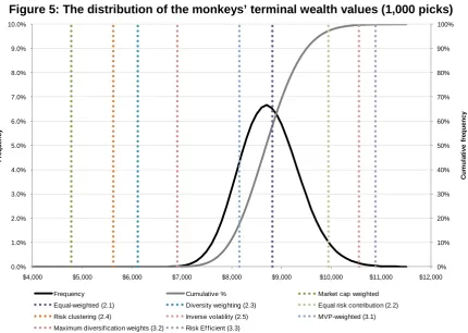
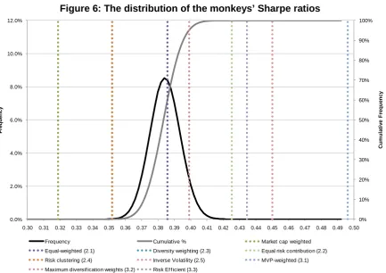
describe as “heuristic”. The second set are based upon “optimisation techniques”, since they all require the maximisation or minimisation of some mathematical function subject to a set of constraints to derive the constituent weights. We find that all of the alternative indices considered here would have produced a better risk-adjusted performance than could have been achieved by having a passive exposure to a market capitalisation-weighted index. However, the most important result of our work stems from our ten million Monte Carlo simulations. We find that choosing constituent weights randomly, that is, applying weights that could have been chosen by monkeys, would also have produced a far better risk-adjusted performance than that produced by a cap-weighted scheme.

3

1. Introduction

The practice of investing in equity portfolios that are benchmarked against Market-cap weighted indices is very common. This choice of this index weighting scheme is particularly relevant to those investors that choose to track such indices passively. But this choice is also of relevance to those investors that employ active fund managers benchmarked against these indices since the performance and the risk profile of these active managers is usually very closely related to the indices. In this paper we provide a thorough evaluation of two subsets of equity index weighting schemes where the weights of individual equities are determined either by simple, heuristic rules of thumb, or are determined by processes that

use comparatively more demanding optimisation techniques2.

For both sets of alternative indices we calculate the performance that investors would have experienced had they adopted any one of these approaches to the construction of portfolios comprising US equities over this period. By using the same, rich dataset we are able to

compare ‘apples with apples’ and to make definitive statements about the differences in the

constituent characteristics and performances of this range of alternatives.

We find that all of the alternative indices considered here would have produced a better risk-adjusted performance than could have been achieved by having a passive exposure to a market-capitalisation weighted index. However, the most important result of our work stems

from our ten million Monte Carlo simulations. We find that choosing constituent weights

randomly, that is, applying weights that could have been chosen by monkeys, would also have produced a far better risk-adjusted performance than that produced by a cap-weighted scheme.

The rest of this report is organised as follows: in section 2 we outline the essential features of a set of heuristic alternative index construction techniques, while in section 3 we review three more techniques which can only be implemented by using optimisation routines; in Section 4 we outline the data that we use to compare the various index construction methods and also the portfolio construction technique that we use; in section 5 we report the main results and index performance statistics; in Section 6 we take a closer look at the source of the performance differences between the indices; in Section 7, we undertake some Monte Carlo experiments to determine how much of the performance of the indices is due to luck and how much to ‘design’; in Section 8 we consider how the use of a simple timing indicator can improve the risk-adjusted performance of the indices; in section 9 we consider the possible impact of transactions costs on our results; and finally Section 10 concludes the paper.

2. Heuristic index construction techniques – defining the weights

The benchmark: Market-capitalisation weights

The focus of this paper is the performance of the Market-cap weighted approach to indexing equities. Of course there are a number of very familiar indices of this kind, such as the S&P 500 Composite and FTSE-100 indices. However, so that we can make fair comparisons, rather than using these familiar indices as the basis for the comparisons of alternative approaches to equity index constructions, we calculate our own Market-cap weighted index using the same stock universe that we use to construct the various alternatives. The weight of each stock in the Market-cap weighted index that we use here is calculated in the

2

4 conventional manner: the weight of each stock is equal to its Market-capitalization divided by the sum of the Market-capitalisation of all of the other stocks in our chosen universe of 1,000 stocks.

It is has often been suggested that a Market-cap based approach to equity index weights is ‘theoretically’ consistent with the Capital Asset Pricing Model (CAPM), and that such a

portfolio should, if the market is efficient, be ‘mean variance efficient’. That is, any portfolio

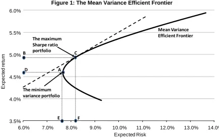
constructed on this basis should have the highest expected return of any set of portfolios with the same expected risk, in turn meaning that it would be impossible to achieve a higher expected return from another portfolio with the same expected risk. A stylised representation of a mean-variance efficient frontier is shown in Figure 1. Any combination of securities that have an expected return and risk combination that means that they plot on the upper portion of this frontier, is said to be mean-variance efficient.

Figure 1: The Mean Variance Efficient Frontier

3.5% 4.0% 4.5% 5.0% 5.5% 6.0%

6.0% 7.0% 8.0% 9.0% 10.0% 11.0% 12.0% 13.0% 14.0%

E

x

pec

te

d r

et

ur

n

Expected Risk

The minimum variance portfolio

The maximum Sharpe ratio portfolio

B C

D A

E F

Mean Variance Efficient Frontier

However, it is simply not true that a Market-cap weighted index will plot on this frontier.

There is no ex ante reason why, for example, a Market-cap weighted portfolio of US equities

should be either mean-variance efficient in a global sense, or consistent with the CAPM in any sense. But most investors that invest on a Market-cap weighted basis do not do so because they think it is theoretically consistent anyway, they do so for the many convenient reasons outlined in last summer’s report.

2.1 Equal weights

5

2.2 Diversity weights

Equally-weighted equity index constituents clearly avoids the problem of concentration that arises from the use of Market-cap weights, but with the potential for increasing positions in less liquid stocks (depending upon the stock universe under consideration of course). A practical approach to this issue might involve setting a cap on the market value of any particular stock in a market- cap weighted index. And redistributing the weight of the largest stocks above this ceiling equally amongst the remaining index constituents. Essentially this approach to index construction combines features of both the Market-cap weighting approach, subject to a maximum constituent weight, and the equal weighting approach. Of course the higher the ceiling of the constituent weight the closer the index will be to a pure Market-cap based index, while the lower it is the closer it will be to an equally weighted index.

To this extent this blending of Market-cap and equal weights is the principle behind the Diversity Weighting approach to index construction. This approach was first proposed by

Fernholz et al (1998). Effectively it involves raising the Market-cap weight (w) of each

constituent by the value p, that is wp, where p is bounded between 1 and 0. The weight of

each index constituent is then calculated by dividing its wp weight by the sum of all wps of all

of the constituents in the index. When p is set to 1 then the constituent weights are equal to Market-cap weights and when p is set to 0 the weights are equivalent to equal weights.

To demonstrate how it works consider Table 1. Column 2 shows the market values of 5 hypothetical stocks. Each successive column shows the value of the diversity weights as we change the parameter p, shown in the parentheses in row 1 of the table. The third column shows that the weights are equivalent to Market-cap weights when p is set equal to 1. For example for stock A, (100/185) x 100% = 54.1%. When p is set to 0 (column 7), the weights all equal 20%. As demonstrated in the table, the lower the value of p the closer the constituent weights to equality.

Table 1:

An example of Diversity Weighting for an index with five stocks

Market cap MCW (1) DW (0.75) DW (0.50) DW (0.25) EW (0) Stock A 100 54.1% 44.9% 35.8% 27.3% 20%

Stock B 35 18.9% 20.4% 21.2% 21.0% 20%

Stock C 15 8.1% 10.8% 13.9% 17.0% 20%

Stock D 10 5.4% 8.0% 11.3% 15.4% 20%

Stock E 25 13.5% 15.9% 17.9% 19.3% 20%

185 100% 100% 100% 100% 100%

So this leaves one question: what value of p should we use? In their initial work Fernholz et

al (1998) used a value of p equal to 0.76. In their tests of this approach to index construction

Chow et al (2011) also report results with p set to 0.76; so for purposes of comparison in our

main results we also set p equal to 0.76.

2.3 Inverse volatility

6

demonstrated that low volatility stocks tended to outperform high volatility stocks3. More

recently there has been growing interest in ‘low volatility investing’, and we therefore felt that it was worth exploring the consequences of creating an index where we assigned a greater weight to stocks with relatively low return volatility. To do this we began by estimating the standard deviation of the return of each stock in the universe using five years of monthly data. We then calculate the inverse of this value, so that the stock with the lowest volatility will have the highest inverted volatility. We then simply summed these inverted standard deviations. The weight of stock i is then calculated by dividing the inverse of its return standard deviation by the total inverted return standard deviation. This process therefore assigns the biggest weight to the stock with the lowest volatility, and the lowest weight to the stock with the highest return volatility.

2.4 Equal risk contribution weights

Equally weighting an index as a rule of thumb (which is one definition of a ‘heuristic’

approach), would seem to be as sensible as assigning weights based on

Market-capitalization, at least in an ex ante sense. But an equal weighting in terms of

Market-capitalisation does not necessarily mean that the contribution to the volatility of the portfolio will be equal. The index weight of each stock in an equally weighted index of 100 stocks will be 1%. But those stocks with relatively high levels of volatility will then contribute more to the overall volatility of the index than those stocks with lower volatility.

This will only “tend” to be true, because it is not only the individual stock’s volatility that will matter, but also the way in which the returns on that stock correlate with the other 99 stocks. Therefore an alternative heuristic approach to the equally–weighted approach to determining index weights would be to use measures of past stock return volatilities and correlations to choose weights such that the contribution of each stock to the risk of the overall portfolio is

equal4 (see Maillard et al (2008)). That is, so that in a 100 stock index each stock

contributes 1% of the index’s total volatility.

2.5 Risk clustering weights

The final heuristic approach that we consider to index construction involves the equal weighting, not of individual equity constituents, but instead the equal weighting of “risk clusters”. With this technique each risk cluster comprises market value weighted constituents that have similar risk characteristics. The identification of risk clusters normally relies on fairly complex statistical procedures. But a very simplified version of this process might be to split a stock universe into its sectoral components, that is, Industrials, Financials, Consumer Discretionary etc, then to construct an index where each sector has an equal weight, but within each sector the constituents are Market-cap weighted. So, to some extent, this process would involve equally weighting a set of Market-cap weighted sectoral indices to create one, ‘risk clustered’ index.

The risk clustering approach to index construction is similar at least in spirit to the approach outline above. It begins with the identification of equity sectors. For a risk clustering index focusing on a single market, the sectors will each represent a Market-cap weighted component of the related stock market. However, for a risk clustering index spanning a number of markets there is a second, country dimension to the sector definitions so, for

3

Haugen, Robert A., and James Heins. 1975. “Risk and Rate of Return on Financial Assets: Some Old Wine in New Bottles,” Journal of Financial and Quantitative Analysis, vol. 10 no. 5 (December): 775–784.

4

See Maillard, Sébastien, Roncalli, Thierry and Teiletche, Jerome, On the Properties of Equally-Weighted Risk Contributions Portfolios (September 22, 2008). Available at:

7 example, as well as there being a consumer discretionary sector for the US, there will be other consumer discretionary sectors for each other market, for the UK, for France, for Japan etc.

Once all of the sectors are identified, statistical techniques are applied to identify clusters of sectors that are similar. This is a purely statistical process involving no economic or finance related input. However, before the statistical procedure can begin the index constructor has to specify the number of clusters that they want to construct. Once the desired number of risk clusters has been identified each sector within a risk cluster is given an equal weight, and then finally each risk cluster itself is given an equal weight so that it comprises the risk cluster index.

In our work we apply this approach to US stocks and identify 30 US industrial sectors. From

these sectors we create ten risk clusters using a k-mediod5 partitioning technique, and

create the index from these clusters following the process explained above.

2.6 Summary

Each of the alternative equity index weighting schemes considered above seek to reduce the sorts of concentration risks that can arise from a straightforward application of Market-cap weights. None have a basis in finance theory, and there is no ex-ante reason why investors should expect one to perform better than the other. Furthermore, with the exception of the partitioning technique needed for risk clustering, all of the alternatives are relatively simple to understand. The next set of alternatives that we consider require the application of optimisation techniques.

3. Optimization-based index construction techniques6

The process of optimisation involves trying to achieve some goal, which could be to find the maximum or minimum value of a variable, subject to certain constraints. So, for example, one could estimate the expected returns, expected volatilities and expected correlations relating to a universe of stocks. Given these inputs it is then a relatively simple computational task to find the portfolio weights from this universe that would give the highest expected return for a pre-specified level of expected risk. The goal in this case is the “highest return possible”, while the constraint is that this return should be achieved for the “lowest amount of expected risk” possible. In fact when we take that set of stocks and find the highest return portfolios for every level of expected risk, we obtain the mean-variance efficient frontier shown in Figure 1. Each portfolio that plots on the frontier is the optimised portfolio with the highest Sharpe ratio for each level of expected risk.

3.1 Minimum variance weights

When constructing the mean variance frontier using optimisation techniques, point A in Figure 1 represents the lowest level of expected risk that can be achieved by combining all the securities in the chosen universe. The optimiser chooses weights for each stock in this universe so that the expected risk (point E) is as low as possible, where the weights are all constrained to be between 0% and 100%, that is, no short positions are allowed. The

5

For those that really wish to learn more about this technique see Kaufman, L. and Rousseeuw, P.J. (1987), Clustering by means of Medoids, in Statistical Data Analysis Based on the L1-Norm and Related Methods, edited by Y. Dodge, North-Holland, 405–416.

6

To estimate the relevant variance-covariance matrices we used five years of historic data and applied the shrinkage technique outlined in Ledoit, O. and Wolf, M. (2004). Honey, I shrunk the sample covariance matrix. Journal of Portfolio Management 30, Volume 4, 110-119. We used the Matlab code from Michael Wolf’s website, which can be found at:

8 expected return on this portfolio (point D) is a function of the weighted average returns of the individual equities. As can be seen, the expected return on this portfolio is lower than any portfolio located on the upper portion (the efficient portion) of the efficient frontier. But under what circumstances would it make sense to use MVP index weights?

One possible instance where constructing an index, or portfolio on a MVP basis might make sense, would be if one took the view that stock returns are so unforecastable that one may as well assume that the expected return on each stock is identical. In this case the mean-variance optimiser would produce not a pleasing looking curve as in Figure 1, but instead a single point within the expected return, expected risk plane, where the expected risk (volatility) would be the minimum achievable level of risk from combining these stocks; and where the expected return on the index would be the same as the return expected on each one of the stocks in this universe.

At each index reconstruction date one could create an MVP index by finding the weights that satisfy this simple optimisation problem. However, in practice if this process is applied in a completely unconstrained manner then the index can often comprise only a very small proportion of stocks, where the remainder are assigned a weight of 0%. Given that concentration risk is one of the key drawbacks of Market-cap based weights it would be equally unappealing to some investors to have a concentrated portfolio constructed from the MVP process. Therefore we construct both an unconstrained MVP-based equity index and a constrained one where the maximum constituent weight is set at 1%, and then again at 5%.

Constructing a MVP-based equity index avoids the knotty problem of having to forecast

equity returns, but it is not obvious why investors would want to construct an index which, ex

ante at least, will give them the most ‘efficient’ but lowest possible return. If the expected

return on all stocks are not identical – which seems very likely – then there exists the prospect of moving along the mean-variance efficient frontier to achieve higher returns, though at the expense of taking on more risk. But to construct a full mean variance frontier, rather than just the MVP would require the index constructor to forecast returns on all of the index constituents. Since it is very likely that any two equity analysts will provide different return forecasts on the just one stock, this would seem to be an impossible task. However, two of the alternative index construction techniques that we examine do offer a solution to

this problem. The first of these is the Maximum Diversification approach proposed by

Choueifaty and Coignard (2008)7, while the second is the Risk Efficient technique proposed

by Amenc et al (2010)8.

3.2 Maximum Diversification weights

Choueifaty and Coignard postulate that the expected return on individual stocks is directly proportional to their volatility. That is, the more volatile a stock’s return the higher will be its average return. Given this heuristic assumption Choueifaty and Coignard then use optimisation techniques to identify the weights of individual equity components that generate the highest Sharpe ratio. On the stylised efficient frontier shown in Figure 1, point C represents the point on the frontier that has the highest Sharpe ratio, that is, that point on the frontier where the ratio of the excess expected return (point B) relative to expected risk (point F) is greatest.

7

Choueifaty, Y. and Y. Coignard (2008), Toward maximum diversification, Journal of Portfolio Management, vol. 35, 40-51.

8 _A

9 The numerator in the Sharpe ratio is the weighted average volatility of the index components (the ‘expected’ index return), while the denominator is the standard deviation of the ‘expected return’ of the weighted index. As with the MVP index construction method, the lower bound for any constituent weight is set to 0% so that the index does not consist of short positions. And to stop the optimiser applying non-zero weights to only a few stocks Choueifaty and Coignard set the maximum index weight to 10%.

3.3 Risk Efficient weights

Amenc et al propose an index construction approach that is similar, at least in spirit, to the

Maximum Diversification technique. However, instead of assuming or postulating, that the expected return on a stock is directly proportional to its volatility, they instead suggest that it is proportional to the downside deviation of the stock’s return – another heuristic assumption.

The downside deviation of a stock’s return is calculated in much the same way as one would calculate its standard deviation. But standard deviation gives the same weight to positive as it does to negative returns. By contrast, downside deviation is calculated using only negative stock returns. So for example, in the extreme case, if the set of monthly returns on a stock are all positive, the stock’s downside deviation will be 0%. However, unless this set of positive monthly returns are identical, the standard deviation of the stock’s returns will be positive. Downside deviation focuses attention on negative returns so, other things equal, the greater their frequency and size, the higher will be the stock’s measured return downside deviation.

To construct a Risk Efficient index Amenc et al propose a two stage process. First, the semi

deviation of each stock is calculated. Then on the basis of these estimates, the stocks are grouped into deciles so that the 10% of stocks with the largest downside deviation comprise the first decile; the 10% with the next highest downside deviation comprise the second decile and so on, until ten deciles are identified. The median downside deviation for each decile is then calculated and this value is then assigned to each stock in its decile as the proxy for the expected return of that stock. The second stage then involves finding the portfolio with the maximum expected return (proxied by the median downside deviation of each stock’s decile) with the lowest portfolio return standard deviation.

Again, to prevent the optimiser from creating a portfolio with concentrated single stock

exposures, Amenc et al impose restrictions on the constituent weights that might otherwise

be chosen by the optimiser. The weight limits are as follows:

lower limit = 1/(λ x N) x 100%

upper limit = λ/N x 100%

where N represents the total number of stocks under consideration and where λ is a free

parameter. If N equals 1,000 and λ is set equal to 2, then the limits on each index

component would be:

lower limit = 1/(2x1,000) x 100% = 0.05%

upper limit = (2/1,000) x 100% = 0.2%

The eagle-eyed will have noticed that if λ is set equal to 1, then all constituent index weights

would be equal to 1/N, that is, the index constituents would be equally-weighted. In our

replication work we construct the Risk Efficient index from a universe of 1,000 stocks with λ

10

3.4 Summary

The alternative index weights based upon optimisation routines might seem more ‘scientific’ than the heuristic alternatives reviewed in Section 2, but none of them are consistent with modern portfolio theory. To be consistent with theory the MVP approach would necessitate that the expected returns on all stocks were identical. With regard to the Maximum Diversification and Risk Efficient approaches, both suggest that investors are rewarded for taking on stock specific risk, that is, the higher the risk either calculated as standard deviation or downside deviation, the higher the expected return, and yet we know that this risk can be diversified away within any randomly chosen portfolio with sufficiently large number of constituents. Second the basis of both these approaches, which both seek to identify a maximum Sharpe ratio is a rather arbitrary assumption about the relationship between expected returns and risk.

Once again, ex ante, there is no reason to expect one approach to be better than the other,

or indeed any better than those approaches outlined in Section 2. The value of any of these alternative approaches to indexing is an empirical issue.

4. Data and portfolio construction methodology

4.1 Data

The data that we use to test the performance of all of the alternative index construction

techniques outlined in Sections 2 and 3 of this report were collected from the CRSP9 data

files. This dataset contains the end month, total returns on all US equities quoted on the

NYSE, Amex and NASDAQ stock exchanges. In keeping with previous work in this area10,

we excluded Exchange Traded Funds (ETFs) and American Depository Receipts (ADRs). The sample period that we use spans the period from January 1968 to December 2011.

Again, in keeping with similar analysis in this area, we choose an index construction methodology which, for the first full year in our sample, involves identifying the 1,000 largest stocks by Market-capitalisation as at December of that year that have five full years of return history, and where Market-capitalisation is calculated as the stock’s share price multiplied by the number of outstanding ordinary shares. We then apply the weights to these thousand stocks which are suggested by the various strategies that we reviewed in Sections 2 and 3. The performance of the relevant index, and sub-components of each alternative index were then collated. This process is repeated in the following year, where we again identify the 1,000 largest US stocks in December of that year that have five full years of return history, repeating both the index calculation exercise and the collation of relevant return data. This process eventually produces a continuous portfolio, representative of each index construction methodology, plus sub-components of this index, from January 1969 to December 2011. The process means that the constituent weights of each methodology are calculated at the end of each year, so that each index itself is rebalanced annually.

As well as calculating the performance of these proxies for alternative indices using the usual performance statistics, such as the Sharpe ratio etc, we also collect data on the characteristics of the index constituents.

4.2 Examining the Maximum Diversification and Risk Efficient heuristic return assumptions

Choueifaty and Coignard postulate that the more volatile a stock’s return the higher will be its average return. However, Figure 2 offers very little support for this idea. Each year we

9

The Chicago Booth Centre for Research in Securities Prices (CRSP) historic database provide US daily corporate actions, price, volume, return, and shares outstanding data for securities with primary listings on the NYSE, NASDAQ, Amex, and ARCA exchanges.

10

11 estimated the volatility of the stocks in our database, the ten percent of stocks with the lowest historic volatility (based on 60 months of data) were placed in decile 1; the ten percent of stocks with the next lowest historic volatility (based on 60 months of data) were placed in decile 2, etc. We repeated this process for every year in our 45 year sample, until we had produced ten equity portfolios ranked by volatility. Each bar in the Figure represents the annualised return of these volatility-ranked deciles. As the Figure shows, if anything high volatility tends to lead to lower annualised returns.

Figure 2: The relationship between volatility and returns

2% 4% 6% 8% 10% 12%

1 2 3 4 5 6 7 8 9 10

A

n

n

u

a

li

s

e

d

r

e

tu

rn

Low volatility (1) to high volatility (10) deciles

Amenc et al postulate that the return over time on a stock is directly proportional to the

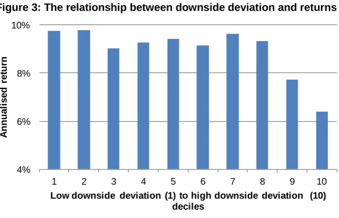
downside deviation of its return. We also tested this proposition using the same methodology that generated Figure 2, but where we used the downside deviation of a stock’s return for the ranking process instead of its standard deviation. The results are shown in Figure 3. Once again, if anything, the higher the downside deviation of a stock the lower is its subsequent average return.

Figure 3: The relationship between downside deviation and returns

4% 6% 8% 10%

1 2 3 4 5 6 7 8 9 10

A

n

n

u

a

li

s

e

d

r

e

tu

rn

12

5. Main results

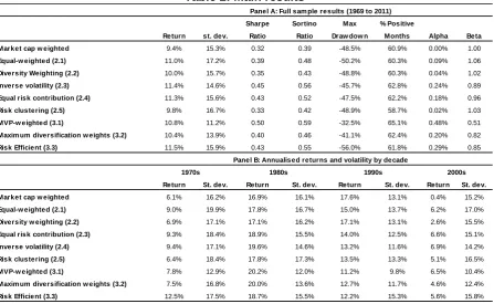
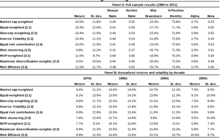
Table 2 presents the performance statistics of each of the index construction methods described in Sections 2 and 3, using the full sample period, and the annual rebalancing methodology described in Section 4.

5.1 Returns

The second column in Panel A of Table 2 presents the average, annualised returns on each of the index construction methodologies. The first point to notice is that the Market-cap weighted approach produces the lowest return of 9.4%, over the full sample. The highest returns are achieved by the Inverse volatility and Risk Efficient approaches, which generate annualised returns of 11.4% and 11.5% respectively. The risk efficient index approach presented in the Table is produced with the constraint that no index constituent has a greater than 5% weight in the index. We have imposed the same constraint on the minimum variance and maximum diversification techniques to make them broadly comparable. The

risk efficient index approach still produces the highest return over this sample period11. The

worst performance is produced by the risk clustering index, however, it is probably fair to say that this approach might be better suited to an international dataset rather than to one with only one country. Column 3 in Panel A of Table 2 presents the annualised standard deviations of the returns of each index. By this measure the index that generated the highest volatility was the Equally Weighted index (17.2%). The index that produced the lowest volatility by far was the Minimum Variance Portfolio index (11.2%). The volatility of the returns of the remaining indices range between 13.9% and 16.7%. The volatility of the Market-cap index is neither relatively high nor low.

Table 2: Main results

Sharpe Sortino Max % Positive

Return st. dev. Ratio Ratio Draw dow n Months Alpha Beta

Market cap w eighted 9.4% 15.3% 0.32 0.39 -48.5% 60.9% 0.00% 1.00

Equal-w eighted (2.1) 11.0% 17.2% 0.39 0.48 -50.2% 60.3% 0.09% 1.06

Diversity Weighting (2.2) 10.0% 15.7% 0.35 0.43 -48.8% 60.3% 0.04% 1.02

Inverse volatility (2.3) 11.4% 14.6% 0.45 0.56 -45.7% 62.8% 0.24% 0.89

Equal risk contribution (2.4) 11.3% 15.6% 0.43 0.52 -47.5% 62.2% 0.18% 0.96

Risk clustering (2.5) 9.8% 16.7% 0.33 0.42 -48.9% 58.7% 0.02% 1.03

MVP-w eighted (3.1) 10.8% 11.2% 0.50 0.59 -32.5% 65.1% 0.48% 0.51

Maxim um diversification w eights (3.2) 10.4% 13.9% 0.40 0.46 -41.1% 62.4% 0.20% 0.82

Risk Efficient (3.3) 11.5% 15.9% 0.43 0.55 -56.0% 61.8% 0.29% 0.85

Return St. dev. Return St. dev. Return St. dev. Return St. dev.

Market cap w eighted 6.1% 16.2% 16.9% 16.1% 17.6% 13.1% 0.4% 15.2%

Equal-w eighted (2.1) 9.0% 19.9% 17.8% 16.7% 15.0% 13.7% 6.2% 17.0%

Diversity w eighting (2.2) 6.9% 17.1% 17.1% 16.2% 17.1% 13.1% 2.6% 15.5%

Equal risk contribution (2.3) 9.3% 18.4% 18.9% 15.5% 14.0% 12.5% 6.6% 15.1%

Inverse volatility (2.4) 9.4% 17.1% 19.6% 14.6% 13.2% 11.6% 6.9% 14.2%

Risk clustering (2.5) 6.4% 18.4% 17.8% 17.3% 13.5% 13.3% 5.1% 16.5%

MVP-w eighted (3.1) 7.8% 12.9% 20.2% 12.0% 11.2% 9.8% 6.5% 10.4%

Maxim um diversification w eights (3.2) 7.5% 16.8% 20.0% 13.6% 12.7% 11.7% 4.6% 12.4%

Risk Efficient (3.3) 12.5% 17.5% 18.7% 15.5% 12.2% 15.3% 5.6% 15.8%

1970s 1980s 1990s 2000s

Panel A: Full sam ple results (1969 to 2011)

Panel B: Annualised returns and volatility by decade

Notes: The figures in parentheses in column 1 of the table relate to the section in the report where the index construction method is described. Returns and standard deviations of returns are all annualised figures. The alphas presented in column 8 are monthly. For the Diversity Weighting index (2.2) we set the parameter p equal to 0.76. For purposes of comparison we set the maximum constituent weight to 5% for the Minimum Variance index (3.1), the Maximum Diversification index (3.2) and for the Risk Efficient Index (3.3).

11

13 Panel B of Table 3 breaks down the annualised return and annualised standard deviation of return of each technique by decade. The Market-cap weighted approach is the worst performing index construction technique in the 1970s, but it performs particularly badly in the 2000s. Indeed the annualised performance of 0.44% in the Noughties appears to be a

substantial outlier. By contrast the 1990s appears to have been the ‘Market-cap decade’,

where this index technique comfortably outperformed most other techniques with an annualised return of 17.59%, compared with the Risk Efficient technique – the best performing technique of the whole sample – which produced a relatively modest 12.2% over the same period. Perhaps the most notable feature of the sub-sample analysis of volatility in Panel B is that over each decade the index with the lowest annualised standard deviation is the Minimum Variance Portfolio index.

5.2 Risk ratios

But of course it is not only return that matters. Panel A of Table 2 also presents a range of risk statistics. We calculated the very familiar Sharpe ratio for each index (Si), which is written as:

Si = (Ri-Rf)/σi

where Ri is the average return on the index, rf is a proxy for the risk free rate of interest, in

this case the average return on US T-bills; and σi is the standard deviation of the returns on

index i. The higher this ratio, the higher has been the return relative to each unit of risk. The higher the Sharpe ratio the better. The lowest Sharpe ratio is produced by the Market-cap approach to indexation. The highest is produced by the minimum variance index (MVP) approach. We also calculated the less familiar Sortino ratio which is based upon the semi deviation, σs-d,i, of index i’s returns, rather than on the full range of returns, in other words it is

only based upon negative returns and disregards all positive returns:

Si = (Ri-Rf)/σs-d,i

However, the results are broadly unchanged: the Market-cap weighting technique generates the lowest risk-adjusted returns while the MVP approach generates the best.

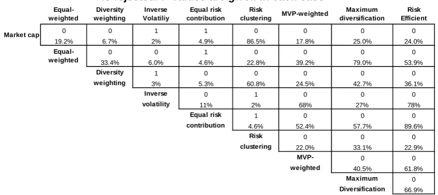
Table 3: Test of null hypothesis that Sharpe ratios are equal. A value of 1 means null is rejected. P-values are given in each case

Equal-weighted Diversity weighting Inverse Volatiliy Equal risk contribution Risk clustering MVP-weighted Maximum diversification Risk Efficient

0 0 1 1 0 0 0 0

19.2% 6.7% 2% 4.9% 86.5% 17.8% 25.0% 24.0%

0 0 1 0 0 0 0

33.4% 6.0% 4.6% 22.8% 39.2% 79.0% 53.9%

Diversity 1 0 0 0 0 0

weighting 3% 5.3% 60.8% 24.5% 42.7% 36.1%

Inverse 0 1 0 0 0

volatility 11% 2% 68% 27% 78%

Equal risk 1 0 0 0

contribution 4.6% 52.4% 57.7% 89.6%

Risk 0 0 0

clustering 22.0% 33.1% 22.9%

MVP- 0 0

weighted 40.5% 61.8%

Maximum 0

Diversification 66.9%

Market cap

Equal-weighted

14 But the Sharpe ratio of one index may be higher than that of another, simply by chance. To determine how different the Sharpe ratios were from one another we performed a set of

complex statistical techniques12 to determine the differences. The results are shown in

Table 3. Each cell in the table shows the results of the test of the difference between the full sample Sharpe ratios of each pair of indices. A value of 1 in the cell is a rejection of the null hypothesis that the Sharpe ratios are the same at the 95% confidence level. In each cell we have also presented the relevant p-values.

Table 3 shows that there are only six instances where the pairs of Sharpe ratios prove to significantly different from one another at the 95% level of confidence. With regard to our main focus here, although the results presented in Table 2 showed that all eight of the alternative equity weighting schemes produced higher Sharpe ratios than the Market-cap index, Table 3 shows that only two of them – Inverse Volatility and Equal Risk Contribution – appear to produce a higher Sharpe ratio than the Market-cap index at the 95% level of confidence. However, the table does show that the Diversity Weighting index produced a higher Sharpe ratio than the Market-cap index at the 90% confidence level. With regard to the remaining alternative indices we cannot say with any statistical certainty that their Sharpe ratios are different from the one produced by the Market-cap index.

5.3 “Systematic” risk

We also calculated the alpha and beta of each index, where the market return was proxied by the Market-cap index. This is why the alpha and beta of the Market-cap index are 0.0 and 1.0 respectively. In other words the remaining alphas and betas are estimated relative to the market index.

First, all of the alternative indices produce a positive alpha. In fact, relative to the Market-cap weighted index, they all produce positive alphas over a long period of time, a performance of which many active fund managers would have been proud. The MVP index construction technique generates the highest alpha over this period of 0.48% per month. The smallest alpha of 0.02% was generated by the risk clustering alternative index.

Second, the ‘systematic risk’ of each index is also expressed relative to the Market-cap

index. For the Equal-weighted, Equal Risk Contribution, Diversity Weighting and Risk Clustering indices the betas are all very close to one, indicating a relatively close average relationship with the Market-cap weighted index. However, the beta coefficients on the Inverse Volatility index and on the three optimised indices are much lower than one. In particular, the beta on the MVP-weighted index is 0.51. These results indicate that these indices, and in particular the MVP index seem to be deriving their returns from a different source than the Market-cap index.

5.4 Tail Risk

For many institutional investors, and in particular for Defined Benefit pension schemes, but also for very risk averse retail investors including those approaching retirement, avoiding significant declines in the value of their equity portfolios is crucial. Column 5 in Panel A of Table 2 presents the maximum drawdown statistics for each index. This statistic is calculated as the largest peak to trough decline in each index in percentage terms. The index calculation methodology with the lowest maximum drawdown is MVP, where the largest peak to trough fall of this index between 1969 and 2011 was 32.5%. The Maximum

15 Diversification index produced the next best peak to trough fall of 41.1%. The worst maximum drawdown statistic is produced by the Risk Efficient index, where the maximum peak to trough fall was 56.0% over the period. The remaining indices all experience peak to trough falls between 45% and 50%.

In this regard then the MVP index would have represented an attractive alternative for risk averse investors, particularly when we consider that the annualised returns on this index were well above those of the Market-cap based index.

5.5 Parameter sensitivity

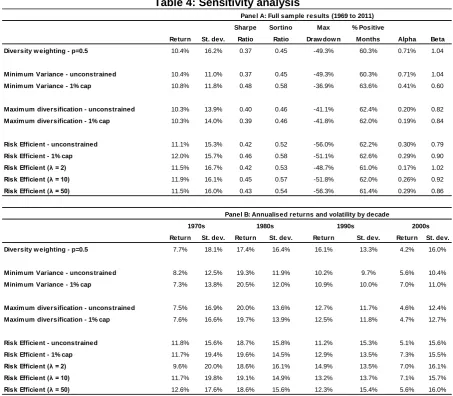
In Table 2 we presented a set of results for alternative indices of US equities. In Table 4 we present a similar set of results for a selection of the indices where the choice of indexing parameter may influence the results. In the first row of Panel A we present the index statistics related to the Diversity Weighting index, but where p is set equal to 0.5 rather than 0.76, as in Table 2. Recall that when p=1.0, the index weights are identical to those of a Market-cap weighted index; and when p=0.0 the weights are equivalent to those of an equally weighted index. 0.5 is exactly half way. The results in Table 5, unsurprisingly then show that the Diversity Weighting index with p=0.5 produces a performance that is closer to that of the equally weighted index than when p=0.76. For example, the annualised return increases from 10.0% to 10.4%.

Of perhaps more interest is the way in which the optimised indices change when the constraints around their constituent weights are changed. In Table 2 , in each case, the maximum constituent weight was set to 5%.

The details of the performance of the MVP index with a 1% constituent cap presented in Table 4, are very similar to those with the 5% constituent cap shown in Table 2. The annualised returns and Sharpe ratios are almost unchanged. However, the performance of the unconstrained equivalent MVP index is worse, in terms of annualised returns, Sharpe ratio and maximum drawdown. This indicates that with a universe of 1,000 stocks a constituent cap can improve the performance of a MVP based index, but that it does not need to be greater than 1.0%.

16

Table 4: Sensitivity analysis

Sharpe Sortino Max % Positive

Return St. dev. Ratio Ratio Draw dow n Months Alpha Beta

Diversity w eighting - p=0.5 10.4% 16.2% 0.37 0.45 -49.3% 60.3% 0.71% 1.04

Minim um Variance - unconstrained 10.4% 11.0% 0.37 0.45 -49.3% 60.3% 0.71% 1.04

Minim um Variance - 1% cap 10.8% 11.8% 0.48 0.58 -36.9% 63.6% 0.41% 0.60

Maxim um diversification - unconstrained 10.3% 13.9% 0.40 0.46 -41.1% 62.4% 0.20% 0.82

Maxim um diversification - 1% cap 10.3% 14.0% 0.39 0.46 -41.8% 62.0% 0.19% 0.84

Risk Efficient - unconstrained 11.1% 15.3% 0.42 0.52 -56.0% 62.2% 0.30% 0.79

Risk Efficient - 1% cap 12.0% 15.7% 0.46 0.58 -51.1% 62.6% 0.29% 0.90

Risk Efficient (λ = 2) 11.5% 16.7% 0.42 0.53 -48.7% 61.0% 0.17% 1.02

Risk Efficient (λ = 10) 11.9% 16.1% 0.45 0.57 -51.8% 62.0% 0.26% 0.92

Risk Efficient (λ = 50) 11.5% 16.0% 0.43 0.54 -56.3% 61.4% 0.29% 0.86

Return St. dev. Return St. dev. Return St. dev. Return St. dev.

Diversity w eighting - p=0.5 7.7% 18.1% 17.4% 16.4% 16.1% 13.3% 4.2% 16.0%

Minim um Variance - unconstrained 8.2% 12.5% 19.3% 11.9% 10.2% 9.7% 5.6% 10.4%

Minim um Variance - 1% cap 7.3% 13.8% 20.5% 12.0% 10.9% 10.0% 7.0% 11.0%

Maxim um diversification - unconstrained 7.5% 16.9% 20.0% 13.6% 12.7% 11.7% 4.6% 12.4%

Maxim um diversification - 1% cap 7.6% 16.6% 19.7% 13.9% 12.5% 11.8% 4.7% 12.7%

Risk Efficient - unconstrained 11.8% 15.6% 18.7% 15.8% 11.2% 15.3% 5.1% 15.6%

Risk Efficient - 1% cap 11.7% 19.4% 19.6% 14.5% 12.9% 13.5% 7.3% 15.5%

Risk Efficient (λ = 2) 9.6% 20.0% 18.6% 16.1% 14.9% 13.5% 7.0% 16.1%

Risk Efficient (λ = 10) 11.7% 19.8% 19.1% 14.9% 13.2% 13.7% 7.1% 15.7%

Risk Efficient (λ = 50) 12.6% 17.6% 18.6% 15.6% 12.3% 15.4% 5.6% 16.0%

1970s 1980s

Panel A: Full sam ple results (1969 to 2011)

Panel B: Annualised returns and volatility by decade

1990s 2000s

Notes: Returns and standard deviations of returns are all annualised figures. The alphas presented in column 8 are monthly.

Table 4 also presents several versions of the Risk Efficient index, an unconstrained one and one with an index constituent cap of 1%, plus three more where lambda is set equal to 2, 10 and 50. First, the unconstrained index underperforms the Risk Efficient index with the 5% constituent cap presented in Table 2, by an annualised 0.4% per annum, but otherwise the performance is very similar. In return terms the best performing Risk Efficient index is the one with a 1% constituent weight cap, which produced an annualised return of 12% and a Sharpe ratio of 0.46.

Of the remaining Risk Efficient indices, which all have the constituent weights constrained by

λ, the differences between them are relatively slight. The highest annualised return and Sharpe ratio occurs when we set λ to 10; while the highest information ratio occurs when we

set λ equal to 2. In their work Amenc et alrecommend setting λ to 2. Overall, and over this particular sample period, we find this index to have the worst risk and return profile, but the difference is so small that it is probably not sufficiently significant to warrant a great deal of consideration.

17

6. A further decomposition of the index returns

The results presented in section 5 indicate that investors that had constructed their equity portfolios along the lines of any of the alternatives considered would generally have outperformed a Market-cap weighted equivalent portfolio over the last four decades. To understand where the performance came from we decomposed the returns of each index in a number of ways.

6.1 The Market-Cap weighted index

For the purposes of comparison, we began by decomposing the returns of the Market-cap index. These results are presented in Appendix 1.

Figure 1A in this appendix shows the three year rolling returns of the index. Figure 1B shows the average weight of the Market-cap index by Beta decile. This figure shows that the Market-cap index has an average 10% weighting in those 10% of stocks with the smallest betas (decile 1), and has the lowest average weighting of 5% to the 10% of stocks with the highest betas (decile 10). Figure 1C presents analogous results with regard to the average weight of the Market-cap index by size. The figure shows that on average just under 60% of its market capitalisation is concentrated in the largest decile of stocks. Figure 1D shows the exposure of the index by book-to-market. In accounting speak, the book value of any asset is recorded on a company’s balance sheet as the original cost of the asset minus depreciation and subject to some other accounting adjustments. A company’s book value is the total value of its booked assets minus its liabilities and also minus intangible assets like ‘goodwill’. We will say more about this exposure in section 6.3, but for the moment we can simply note that the Market-cap weighted index is tilted towards stocks with low book values relative to their market values. Figure 1E shows the Market-cap weighted index’s exposure to high and low momentum stocks. The first momentum decile is comprised of those stocks whose prices have been the worst performing ten percent of stocks over the previous 12 months. Conversely decile 10 is made up of the stocks who have been the top ten percent of stock price performers over the previous 12 months. Again we will say more about the meaning of these momentum exposures in section 6.3, but for now we can see that there is no obvious momentum bias in the Market-cap index. Figure 1F presents the index’s weight by volatility decile. The figure shows, for example, that the Market-cap index has an average 20% weighting to the decile of stocks with the lowest volatility and a 3% weighting towards those stocks with the highest volatility. Figure 1G shows the average monthly return on the Market-cap index in months when the market rises and falls. Finally, Figure 1H shows the average weight of the Market-cap based index by volume decile. On average, and unsurprisingly, the Market-cap index has a weighting of 53% in the top decile of stocks by traded volume, and a combined average of 12% in the five deciles of stocks with the lowest traded volume.

Taken together these results show that a Market-cap index is heavily weighted towards large cap stocks (by design), to the most highly liquid stocks (almost by design), but also to stocks with relatively low return volatility.

Appendices 2 to 8, present the same results for the heuristic and optimised indices discussed in sections 2 and 3, but where the results are expressed relative to the Market-cap index. So, for example, Figure 2A in Appendix 2 shows the three year rolling returns of the Equally Weighted index relative to those generated by the Market-cap index; while Figure 2B in the same appendix, shows the average betas of the Equally Weighted index, by decile, relative to the average betas of the Market-cap index by decile.

6.2 The three year rolling returns of the alternative indices

18 the heuristic indices there appear to be two such periods: in the early part of the 1970s (approximately 1970 to 1975) and during the high tech bubble of the 1990s (approximately 1995 to 2000). There is also a short period beginning in the late 1980s (1988 to 1991) where the Market-cap index outperforms, but only marginally. Generally speaking the optimised indices also underperform between 1970 and 1975, and 1995 to 2000, but also fairly substantially in the 1988 to 1991 period too. The optimised index alternative that performs a little differently is the Risk Efficient index. This index does not underperform in the early 1970s to any noteworthy degree, but underperforms substantially between 1984 and 1987, 1990 and 1992 and then finally between 1995 and 2000.

Of course, past performance is no guarantee of future performance, simply opting for the best performing alternative index is no guarantee of future outperformance, but even if future performance is superior, it seems likely that there could be times when investors could expect to underperform a Market-cap weighted equity index.

6.3 Index factor exposures

The analysis of the performance of equity portfolios often begins by decomposing the returns generated by the portfolio into four, systematic sources of return, that is, estimating how much of the fund’s return was due to its exposure to the ‘market’, to small cap stocks, to stocks with high book-to-market values, or to stocks with relatively high price momentum. The appendices of Figures for each index construction methodology contain information on their exposures to these four factors. Figures B, C, D and E show the index tilts towards market risk (represented by beta), size, book-to-market value and momentum respectively.

6.3.1 The market

According to the Capital Asset Pricing Model (CAPM) the “universe of all tradable assets” is

the only source of undiversifiable, systematic risk. According to the theory over long periods of time, investors should earn a return over and above a cash return, known as a risk premium, simply from being passively exposed to this source of risk. When analysing equity market risk to capture this source of risk, finance researchers and industry practitioners generally use the return on a broad index of equities as a proxy for market risk.

Figure 2B in appendix 2 shows that the Equally Weighted index is overweight the top four high beta deciles relative to the market. The Diversity Weighting index is overweight the higher beta stocks, but only marginally. Equivalent figures for the other heuristic indices shows that the Equal Risk Contribution and Inverse Volatility indices are overweight the decile of stocks with the lowest betas. The pattern of over and underweight beta exposures for the Risk Clustering index indicate a slight bias towards higher beta stocks. Finally, the figures for the three optimised indices show a significant bias towards the ten percent of stocks with the lowest betas or exposure to market risk. The Minimum Variance index is almost 70% overweight this decile of low beta stocks, while the Maximum Diversification and Risk Efficient indices are 42% and 18% overweight this decile of stocks respectively.

These results show that the alternative indices are not all uniformly under or overweight market risk, as represented by beta. But we can at least say that the three optimised indices are uniformly overweight low beta stocks or, alternatively, that they are underweight market risk.

Although the CAPM remains the benchmark model of risk and return, dissatisfaction with the

empirical performance of this model led Fama and French (1993)13

13

Fama, E., and K. French (1993), Common risk factors in the returns on stocks and bonds, Journal of Financial Economics, vol. 33, 3-56.

19 systematic returns were comprised of two further factors: size and book-to-market value. We now discuss the exposure of the indices to these two risk factors.

6.3.2 Size

A number of researchers had previously found that small cap stocks tended to outperform large cap stocks even though the identifiable market risk in the small cap stocks was lower than was evident in the large cap stocks. In other words, there seemed to be a risk premium that could be earned from investing in small cap stocks that was independent of the premium that could be earned from being only exposed to ‘market’ risk.

Figure 2C in appendix 2 shows the relative decile exposures by Market-capitalization for the Equally Weighted index. Unsurprisingly the figure shows that this index is 50% underweight the largest ten percent of stocks. The equivalent figures in the other appendices show that the Equal Risk Contribution and Inverse Volatility indices have similarly-sized underweight positions in the top ten percent of large stocks, 46% and 43% respectively. The Diversity Weighting and Risk Clustering indices are also underweight the largest ten percent of stocks, around 14% and 17% respectively. Finally, the optimised indices all show a significant underweight position in the largest ten percent of stocks, just over 40% in each case.

Another way of looking at the differences in the size of the stocks that comprise each index is shown in Figure 4. This figure shows the average size of each index constituent for each index over 2011. The Market-cap weighted average is clearly largest, but the Diversity weighting index, when p is set equal to 0.76, has an average index constituent approximately 80% of the average size of constituents in the Market-cap based index. The Equal Risk, Equal Risk Contribution, Maximum Diversification and Risk Efficient indices comprise stocks that are on average much smaller than those that comprise the Market-cap index.

Figure 4: Weighted average size of index constituents (2011)

$0 $10 $20 $30 $40 $50 $60 $70 $80 $90

Market cap Equal (2.1) Diversity weighting (2.2) Inverse volatility (2.3) Equal risk contribution (2.4) Risk clustering (2.5)

MVP (3.1) Maximum diversif ication

(3.2)

20

Overall these results indicate that all of the indices are underweight large cap stocks, and therefore could all be said to have a bias towards small cap stocks. This is particularly true of the Equal Risk Contribution, Inverse Volatility and optimised indices.

6.3.3 Book-to-market value

Researchers found that companies with a high book-to-market value tended to outperform those with lower book-to-market value. Fama and French (1993) went further and suggested that book-to-market value was a systematic risk factor. They argued that there was a risk premium that could be earned from passive exposure to stocks with a high book-to-market value. Such stocks are often described as ‘value stocks’ because the price being ‘asked’ for their shares in the market is low relative to their recorded book value, by contrast ‘growth’ stocks tend have very low book-to-market values. Importantly, the book value of a company can often be very different from its market value. For example, the book value of Dot.Com firms in the late 1990s was often very, very small relative to the market value of the same firms. This is because these companies unlike, for example, large manufacturing firms had few assets, but they still had a market price that had been inflated by the irrational exuberance of the time.

Figure 2D in appendix 2 shows the relative decile exposures by book-to-market value for the Equally Weighted index. The figure shows that this index has a mild overweight position in those stocks with a relatively high book-to-market value. The equivalent figures in the appendices indicate that the Diversity Weighting and Inverse Volatility indices also have the same, mild bias towards stocks with a high book-to-market value. By contrast the Risk Clustering index has a slight bias towards stocks with relatively low book-to-market values. With regard to the optimised indices, all three are significantly overweight stocks with high book-to-market values. In particular, the Risk Efficient index is 18% overweight the decile of stocks with the highest book-to-market values.

These results indicate that these alternative indices are generally overweight high book-to-market value stocks relative to the exposure of the Market-cap index.

6.3.4 Momentum

Fama and French (1993) first proposed size and book-to-market value as additional systematic sources of risk and return; in further work in the same spirit, Carhart (1997)

identified yet another factor: momentum14. Carhart argued that there was another premium

available to investors that could be derived from tilting portfolios towards stocks with high price momentum, that is, stocks that had performed relatively well compared with other stocks. Essentially Carhart’s argument was that an additional and independent risk premium could be earned by equity portfolio managers over time that by tilting their portfolios towards stocks that had performed relatively well in the past (usually over the previous 12 months).

Figure 2E in appendix 2 shows the relative decile exposures by momentum for the Equally Weighted index. The over and underweight positions are relatively small, and indicate that this index is overweight both the decile of stocks with the lowest price momentum (decile 1) and that decile of stocks with the highest price momentum (decile 10). The Diversity Weighting and Risk Clustering indices have similar patterns of over and underweight momentum exposures, but which are smaller than those for the Equally-Weighted index. The Equal Risk Contribution and Inverse Volatility indices are both marginally underweight high momentum stocks. With regard to the optimised indices, the Minimum Variance index is underweight both low and high momentum stocks, and therefore overweight the middle momentum deciles (3 to 7). The Maximum Diversification index is overweight the lowest and highest momentum deciles and marginally underweight most of the intervening momentum

14

21 deciles. However, the most significant relative exposure is seen when we consider the Risk Efficient index, which is 18% overweight the decile of stocks with the lowest momentum.

In summary, there does not seem to be an obvious momentum bias in the alternative indices where over and underweights are either relatively small, or balanced at either extreme. The clear exception to this narrative however, is the Risk Efficient index which is quite heavily tilted towards low momentum stocks.

6.3.5 The impact of factor tilts on index returns

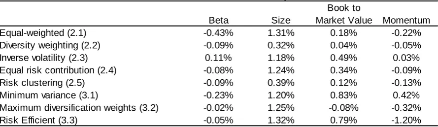
The return produced by a tilt in any equity portfolio or index depends not only on the size of the tilt, as discussed above, but also the return to that tilt. In other words, if there were no additional return available to investors from overweighting small cap stocks over time, it would make little difference to overall performance. To determine the impact of the tilts to the four risk factors for each index and for each factor, we calculated the average value of, for example, being overweight small cap stocks relative to the Market-cap weighted index. These results are shown in Table 5.

Table 5: The ‘returns’ to factor exposures Book to

Beta Size Market Value Momentum

Equal-weighted (2.1) -0.43% 1.31% 0.18% -0.22%

Diversity weighting (2.2) -0.09% 0.32% 0.04% -0.05%

Inverse volatility (2.3) 0.11% 1.18% 0.49% 0.03%

Equal risk contribution (2.4) -0.08% 1.24% 0.34% -0.09%

Risk clustering (2.5) -0.09% 0.39% 0.12% -0.13%

Minimum variance (3.1) -0.23% 1.20% 0.83% 0.42%

Maximum diversification weights (3.2) -0.02% 1.25% -0.08% -0.32%

Risk Efficient (3.3) -0.05% 1.32% 0.79% -1.20%

Notes: The return value in the table represent the annualised difference between the return to the factor exposure of the alternative index relative to the Market-cap index.

The results in Table 6 show that on the whole, the difference in the exposure of the Market-cap index to market risk, represented by beta, and the market risk of most of the alternative indices led to underperformance of the alternatives relative to the Market-cap index. The one exception to this general finding is the Inverse Volatility Index whose relative beta exposure produces a small annualised outperformance over the full sample relative to the Market-cap index of 0.11%. However, in all cases the size tilts of the alternative indices lead to positive performance relative to the Market-cap index. In most cases this outperformance is well above an annualised value of 1.0%. A similar result is seen with regard to book-to-market value. While the impact of the differential exposures to this factor for the Diversity Weighting, Maximum Diversification and Risk Clustering indices is small or negligible, for all of the other indices the exposure to this factor has added quite significantly to the indices returns over time – this is particularly true for the Minimum Variance and Risk Efficient indices. Finally, the differential exposures of the alternative indices to momentum has generally lead to underperformance over time. With regard to this factor the Risk Efficient index underperforms by 1.20% relative to the Market-cap index. The notable exception here is the Minimum Variance index where the annualised outperformance is 0.42%.

22

6.4 Index compositions by total volatility

Some investors are uninterested in the factor decomposition of returns, and instead are more concerned with total volatility, so in addition to decomposing the indices into factor risk buckets, we also decomposed them by total volatility. Each of the appendices for the alternative indices show the decile weights relative to the Market-cap index by total volatility. For example, we can see from appendix 2 Figure 2F that the Equally Weighted index has 7% additional weight to the decile of stocks with the highest volatility. The results show that the Equally Weighted index is generally overweight higher volatility stocks and underweight the lower volatility stocks. The Equal Risk Contribution has a similar weight distribution with regard to total volatility. The Diversity Weighting and Risk Clustering indices also tend to be overweight the more risky stocks – defined by total volatility – and underweight the stocks in the lower risk deciles relative to the Market-cap index. The Inverse Volatility index is underweight by around 6.5% the decile comprising the stocks with the lowest return volatility.

The Minimum Variance Portfolio index, unsurprisingly, is very overweight the lowest risk decile. We find that this index allocates much more to the stocks with the lowest volatility. For example, compared to the Market-cap index, the MVP index has an overweight position of nearly 80% relative to the Market-cap index to the stocks that comprise the lowest decile of total return volatility. The exposures to low volatility stocks should not be a surprise of course, given the construction technique, but the subsequent performance of the index does not appear to be consistent with the empirical prediction of modern portfolio theory, that is that low risk investments over long periods of time should generate relatively low returns. The Maximum Diversification index also produces an interesting allocation to the risk deciles. The distribution of total volatility risk exposures are very similar to those of the Equally Weighted and other heuristic indices, with more exposure to higher volatility stocks and less to lower risk stocks. Finally, the pattern of risk exposures for the Risk Efficient index is also relatively complicated. It produces overweight exposures in the lowest total volatility decile, where the average overweight is 12%. But the index is underweight risk deciles 2 to 5, overweight risk deciles 6 to 9, and then marginally underweight the highest risk decile. However, given that the Risk Efficient index is based upon the semi deviation of stock returns, we have introduced an additional Figure, Figure 9I, for this index breaking down exposure into semi-deviation deciles. The figure shows a different profile, in particular a relatively large overweight position in the top semi-deviation decile of 15%, which is a clear reflection of the index construction methodology.

6.5 Summary

The results presented in this section of the report confirm that alternative weighting schemes would have produced a better risk-adjusted performance for long only US equity investors over the long-term and most strikingly over the Noughties than by weighting constituents by their capitalisation. However, during the long bull market of the 1990s, the Market-cap based index outperformed all the other alternatives. Generally speaking, the alternative indices allocate more weight to stocks with lower realised historic, volatility as well as to smaller stocks and to stocks with high book-to-market values.

In the next section of this paper we try to determine whether the performance differences are due to luck or to intelligent design.

7. Fooled by randomness15

It is unlikely that any of the index construction techniques examined in Section 6 would have produced identical results. In other words, there was always going to be one index that was going to be the best risk-adjusted performer and one that was going to be the worst.

15