One-loop spectroscopy of semiclassically quantized strings: bosonic sector

      

City, University of London Institutional Repository

Citation

: Forini, V., Puletti, V. G. M., Pawellek, M. & Vescovi, E. (2015). One-loop

spectroscopy of semiclassically quantized strings: bosonic sector. Journal of Physics A: Mathematical and Theoretical, 48(8), 085401.. doi: 10.1088/1751-8113/48/8/085401

This is the accepted version of the paper.

This version of the publication may differ from the final published

version.

Permanent repository link:

http://openaccess.city.ac.uk/19725/

Link to published version

: http://dx.doi.org/10.1088/1751-8113/48/8/085401

Copyright and reuse:

City Research Online aims to make research

outputs of City, University of London available to a wider audience.

Copyright and Moral Rights remain with the author(s) and/or copyright

holders. URLs from City Research Online may be freely distributed and

linked to.

City Research Online: http://openaccess.city.ac.uk/ [email protected]

HU-EP-14/29

One-loop spectroscopy of semiclassically

quantized strings: bosonic sector

Valentina Forinia,1, Valentina Giangreco M. Pulettib,c,2, Michael Pawelleka,1 and Edoardo Vescovia,1

a_{Institut f¨ur Physik, Humboldt-Universit¨at zu Berlin, IRIS Adlershof,}

Zum Großen Windkanal 6, 12489 Berlin, Germany

b _{University of Iceland, Science Institute, Dunhaga 3, 107 Reykjavik, Iceland}

c _{Department of Fundamental Physics, Chalmers University of Technology, 412 96 G¨oteborg, Sweden}

Abstract

We make a further step in the analytically exact quantization of spinning string states in semiclassical approximation, by evaluating the exact one-loop partition function for a class of two-spin string solutions for which quadratic fluctuations form a non-trivial system of coupled modes. This is the case of a folded string in theSU(2) sector, in the limit described by a quantum Landau-Lifshitz model. The same applies to the full bosonic sector of fluctuations over the folded spinning string inAdS5with an angular momentum

J inS5. Fluctuations are governed by a special class of fourth-order differential operators, with coefficients being meromorphic functions on the torus, which we are able to solve exactly.

1_{

valentina.forini,michael.pawellek,edoardo.vescovi}@ physik.hu-berlin.de 2

[email protected]

Contents

1 Introduction 2

2 Bosonic fluctuation spectrum for the folded string 5

2.1 Landau-Lifshitz fluctuation spectrum for the SU(2) folded string . . . 5

2.2 Folded string in full bosonic sigma-model . . . 8

3 Fourth order linear differential equations with doubly periodic coefficients 11 3.1 Floquet theory of determinants of fourth order one-dimensional operators . . . 11

3.2 Construction of the solutions: a Hermite-Bethe ansatz . . . 14

3.3 Pole structure . . . 15

3.4 Consistency equations . . . 16

4 Exact bosonic one-loop partition functions for folded string 17 4.1 Exact partition function and one-loop energy for the LL folded string . . . 18

4.2 Folded string in full bosonic sigma-model . . . 22

5 Outlook 24 A The squared Lam´e operator 25 B Landau-Lifshitz SU(2) folded string analysis: details 26 B.1 Spectral domain . . . 26

B.2 A duality property of the LL fourth order differential operator . . . 29

B.3 Finite-gap structure: a microscopical spectral curve . . . 30

B.4 The short string expansion . . . 31

C Folded string in full sigma-model: details 33 C.1 Fluctuation Lagrangian in static gauge . . . 33

C.2 Spectral domain and four linear independent solutions . . . 35

C.3 Theν= 0 limit . . . 38

1

Introduction

i.e. independent on (τ, σ) 3. In this case the semiclassical analysis is highly simplified since the quadratic fluctuation Lagrangian turns out to have also constant coefficients. Then, the operator determinants entering the one-loop partition function are expressed in terms of char-acteristic frequencies which are relatively simple to calculate, and the computation of quantum corrections can be extended to two-loop order4 by standard diagrammatic methods [8,9]5.

Next to simplest cases are “non-homogenous” configurations such as rigid spinning string elliptic solutions, the one-spin folded string solution rotating in AdS5 [15,16] - being a well-known example. This is a stationary soliton problem for which the classical equations of motion consists in a one-dimensional sinh-Gordon equation. In a static gauge where fluctu-ations along the worldsheet directions are set to zero, fluctufluctu-ations turn out to be governed by differential operators of a single-gap Lam´e type [17]. Their determinants can be derived explicitly, leading to an analytically closed integral expression for the full one-loop string par-tition function. Even if the latter is a complicated integral that is not known how to solve explicitly, a merit of this analysis is to facilitate the investigation of various regimes of interest (BPS or far-from-BPS) furnishing a “spectroscopy” much more precise than the one obtained via a perturbative treatment of the fluctuation interactions6. This kind of analysis has been then successfully applied also to the single-spin/parameter case of pulsating string solutions in AdS5 and S5 [19], to open string duals of space-like Wilson loops describing quark-antiquark systems [20] or the so-called [21] Bremsstrahlung function [22] and to the case of backgrounds relevant for the AdS4/CFT3 and AdS3/CFT2 correspondence [23].

In the very general case of non-homogenous solutions with more than one spin, or of single-spin solutions [15,16] in conformal gauge where bosonic fluctuations couple via the Virasoro constraints7, the evaluation of the classical energy requires the diagonalization of highly non-trivial second-order matrix 2d differential operators whose coefficients have a complicated coordinate-dependence. The same is true for fluctuations over open string solutions for which the corresponding cusped Wilson loops have an expectation value which depends on the cusp angle and on another internal angle [22,23]. In all these cases the evaluation of the spectrum has been performed setting to zero one of the spins/parameters involved in the problem -thus falling back in the category discussed above - or resorting to perturbation theory in them [24]. In the case of the single-spin string, it has been possible to evaluate the exact one-loop partition function only in static gauge, where mixing is absent, the equivalence with the partition function in conformal gauge being only shown numerically [17].

3_{Non homogenous solutions can become homogeneous in certain limits, as for the folded string with spinS} inAdS5 and momentumJinS5 in the limitS= √S_λ→ ∞with √_λJ_logS fixed [5,6]. Similarly, in certain cases one can arrange to make the coefficients in the fluctuation Lagrangian constant [7].

4_{Comments on higher-loop calculations in such homogenous case are in [8].}

5_{Another way in which sigma-model perturbation theory has been importantly used in the study of the} integrable structure underlying the AdS/CFT system is the calculation of the worldsheet S-matrix, where results exists at tree-level [10], one-loop [11–13] and two-loop order [12] (for further references see [14]).

6_{See for example, in the large spin limit, the detection of turning-point contributions for the energy of a} single-spin string rotating in AdS5 [17] which are missed by naive perturbation theory, or the possibility to check at high orders the peculiar reciprocity-respecting structure of subleading corrections [18].

Together with the pedagogical motivation of enriching the class of problems that can be solved analytically, the diagonalization of the mixed-modes fluctuation problem for the largest possible set of string configurations is interesting for a number of reasons. First, it provides the natural setup for a detailed comparison between the algebraic curve approach and the direct worldsheet computation of energies for string states, as in some relevant cases passing from one approach to the other implies taking a certain limit which happens to be non-analytic (see discussion in [25,26]). Also, it should help in the solution of existing caveats for the semiclassical analysis in short string regime [25] as well as in the BPS limit of the ABJM Bremsstrahlung function (see discussion in [23,27]). In general, the classical and the expected quantum integrability of the AdS5 ×S5 model should be manifest at the level of small fluctuations near a given solution, regardless how complicated is the latter.

In this paper we make a first step into the exact, detailed solution to the mixed-modes fluctuation spectrum in the case of a non-trivial solitonic configuration, the folded string spinning in S5 with two large angular momenta (J1, J2) - as solution of the Landau-Lifshitz (LL) effective action of [28]8. In that this effective model only involves a part of the bosonic fluctuations modes (those corresponding to theSU(2) sector), therefore missing bosonic and fermionic contributions crucial for the UV finiteness of the quantum result for the energy, it must be equipped with an appropriate regularization. Calculations for the spectrum of the LL model linearized around the folded SU(2) string solution have been made in [24] using operator methods via perturbative evaluation (in the parameter J2/J, J = J1 +J2) of characteristic frequencies, with a sum over them cured via ζ-function regularization. We will evaluate here the exact one-loop effective action over the same solution, regularized by referring the determinants to the limit J2 = 0, which ensures the expected vanishing of the partition function, and proceeding with a ζ-function-inspired regularization of the path integral. The “semiclassically exact analysis” explained below provides an efficient and elegant tool to find in one step the needed spectral information. The result obtained in [24] using perturbation theory up to then-th order means here an n-th order Taylor expansion.

The procedure exploits the integrability of a type of fourth-order linear differential equa-tions with doubly periodic coefficients9_{in terms of which the bosonic fluctuation problem can}

be usefully re-written, and that emerges as the natural generalization of the Lam´e differential equation. Not surprisingly, the same operator appears to govern the mixed-modes bosonic sector of fluctuations for the full AdS5×S5 action when expanded around the folded string solution with non-vanishing AdS3 spin and S1 orbital momentum [16]. As noticed in [23]10, the mixing of bosonic fluctuations here has its supersymmetric counterpart in a non-trivial fermionic mass matrix. Annoyingly, the differential equations governing the fermionic spec-trum do not satisfy the conditions which allowed us to diagonalize the bosonic system, and it is apparently non-trivial to find the necessary generalization of the tools we have developed. We leave the solution of the full string mixed-mode problem for the future 11, but we notice,

8_{See Section2.1below, for a detailed review see [29].} 9

A first attempt to study such kind of equations was done by Mittag-Leffler in [30]. 10

See Appendix D there. 11

as nice byproduct of our analysis, that the tools developed here allow an analytic proof of equivalence between the full (including fermions12_{) exact one-loop partition function for the}

one-spin folded string in conformal and static gauge – a non-trivial statement which in [17] has been verified only numerically.

The paper proceeds as follows. In Section 2 we present the mixed fluctuation problems for the folded string both in the LL and in the full bosonic sectors. In Section 3 we discuss and construct the solutions of the fourth order differential operator governing those spectral problems, which we then solve analytically in Section 4. Three Appendices follow, collecting details on Sections2,3and 4 respectively.

2

Bosonic fluctuation spectrum for the folded string

In this section we consider fluctuations over the classical string configuration representing a string solution folded on itself and rotating with two angular momenta. We present the two examples of coupled system of fluctuations which we will able to diagonalize in Section 4, using the tools presented in Section3.

2.1 Landau-Lifshitz fluctuation spectrum for the SU(2) folded string

The LL effective action, obtained in string theory as a “fast-string” limit of the Polyakov action [28,31], coincides on the gauge theory side with an effective action for the ferromagnetic (bosonic) spin chain in the thermodynamic limit 13. As such, its role as a bridge between quantum string theory and the spin chain description underlying the AdS/CFT Bethe ansatz has been explored in a number of papers (for a review see [29]). We briefly review now the quantum LL approach for the study of a folded 2-spin (J1, J2) string rotating inS5 [24].

The starting point is the LL action for the SU(2) sector [28,31], which is obtained consid-ering a string state whose motion with two large spins is restricted to theS3 _{part ofS}5_{. The} collective “fast” coordinate (β) associated to the total angular momentum is gauged away, while only transverse “slow” coordinates remain to describe the low-energy string motion. This is practically implemented by parameterising the 3-sphere coordinates as X1 +iX2 = U1eiβ, X3+iX4 =U2eiβ, UaUa? = 1, fixing the gauget=τ , pβ = const =J, and rescaling

thet coordinate via ˜λ=λ/J2, which plays the role of an effective parameter. To first order in the ˜λexpansion, one gets [24]

SLL=J

Z

dτ

Z 2π

0 dσ

2πL, L=−iU

?

a∂τUa−

˜ λ

2 |DσUa|

2_+O(˜λ2_{), λ˜≡} λ

J2 , (2.1) DUa=dUa−iCUa, DUa?=dUa?+iCUa?, C =−iUa?dUa .

prescription is given, still correctly reproduce the full string result [4] while neglecting fermionic fluctuations (as well as a part of the bosonic ones).

12

This is because fermions are decoupled in conformal gauge. 13_{The SU(2) sector contains operators of the form Tr(Φ}J1

1 Φ J2

2 ), and the thermodynamic limit reads J =

For the two-spin folded string, describing a closed folded string at the center of AdS, at fixed angle in S5_{, rotating within a S}3 _⊂S5 _{with arbitrary frequencies w}

1, w2, the non-vanishing part of the metric is

ds2 =−dt2+dψ2+ cos2ψ dϕ2₁+ sin2ψ dϕ2₂, (2.2)

and one can write [28]

ds2 = −dt2+dXadXa?, XaXa?= 1, Xa=eiβUa, (2.3)

U1 = cosψ eiϕ, U2 = sinψ e−iϕ, ϕ= ϕ1−ϕ2

2 , β =

ϕ1+ϕ2

2 . (2.4)

Hence, the initial Lagrangian (2.1) becomes [24]

L= cos 2ψϕ˙−λ˜ 2

ψ02+ sin22ψϕ02. (2.5)

The equations of motion following from (2.5) are in terms of a 1d sine-Gordon equation

ψ00+ 2w sin 2ψ= 0, ϕ=−w t , w= w2−w1

2 >0, w = w

˜

λ , (2.6)

ψ02= 2w (cos 2ψ−cos 2ψ0), whose solution can be written as [24]

sinψ(σ) = ksn(Cσ, k2), cosψ(σ) = dn(Cσ, k2), k2 = sin2ψ0, (2.7) √

w = 1 πK(k

2_{), C=} 2

πK(k

2_{) = 2}√_{w ,} E(k2) K(k2) = 1

−J2 J .

The two non-zero spins (J1, J2) are

J1=w1 √

λ

Z 2π

0 dσ 2π cos

2_{ψ , J}

2 =w2 √

λ

Z 2π

0 dσ 2πsin

2_{ψ ,} J1

w1 + J2 w2 =

√

λ . (2.8)

From the Lagrangian (2.5), one can expand around the classical solution

ϕ=ϕcl+

1 √

Jδϕ(τ, σ), ψ=ψcl+ 1 √

Jδψ(τ, σ), (2.9)

obtaining, with the field redefinition

f1 =−sin(2ψcl)δϕ , f2=δψ , (2.10)

and after symmetrization, a fluctuation Lagrangian [2,31,32] which can be usefully written as follows [24]

LLL = 2f2f˙1− 1 2 ˜

λhf₁02+f₂02−V1(σ)f12−V2(σ)f22

i

. (2.11)

Above, in terms of Jacobi functions, one has

V1(σ) = 4w

1 + 4k2−6k2 sn2(Cσ, k2)

, V2(σ) = 4w

1−2k2 sn2(Cσ, k2)

The time-independence of the potentials allows the Fourier-transform∂τ =i ω, after which the

fluctuation equations following from (2.11) form the following non-trivial matrix eigenvalue problem for the characteristic frequenciesω 14

−f₂00(σ)−V2(σ)f2 =iωf1, (2.13)

f₁00(σ) +V1(σ)f1 =iωf2. (2.14)

This system can be solved perturbatively in the elliptic modulusk2 (or equivalently, inJ2/J), and so has been done in [24]. The main result of this paper is theanalytically exact diagonal-ization of this non trivial spectral problem.

To proceed in an analytically exact fashion, we start by decoupling (2.13)-(2.14) into two fourth-order equations

f₂0000+ [V1(σ) +V2(σ)]f200+ 2V20(σ)f20 +

V₂00(σ) +V1(σ)V2(σ)

f2 = 4ω2f2, (2.15) f₁0000+ [V1(σ) +V2(σ)]f100+ 2V10(σ)f10 +

V₁00(σ) +V1(σ)V2(σ)

f1 = 4ω2f1, (2.16)

which, using operator notation

Oi=−

d2

dσ2 −Vi(σ), (2.17)

can be compactly written as

O1O2f2=ω2f2, O2O1f1=ω2f1. (2.18)

The diagonalization of the matrix eigenvalue problem defined by (2.13)-(2.14) is then equiv-alent to the diagonalization of

O_LL = O1 −2∂τ 2∂τ O2

!

, (2.19)

where we used the definitions (2.17).

Defining a new coordinate x=Cσ= 2√wσ, the first equation of the system (2.13)-(2.14) can be rewritten as (we define f2 ≡ f, and omit in the Jacobi functions the dependence on the modulusk2₎

O(4)f(x) = 0, O(4) =∂_x4+ 2 1 + 2k2−4k2sn2(x)∂2_x−8k2sn(x) cn(x) dn(x)∂x+ 1−Ω2,

(2.20) with

Ω = ω 2w ≡

ω π2

2K2 . (2.21)

Equation (2.20) is a fourth-order differential equation with doubly-periodic elliptic coefficient functions 15 with period 2L = 4K (following from the 2π-periodicity of the closed string) and only one regular singular pole, in Fuchsian classification. A first (incomplete) attempt

14

As in [24], the time has been rescaled by ˜λ, which we will restore in the final expressions.

to study this kind of equations was done by Mittag-Leffler 16 in [30], and to our knowledge not much else is known in literature. In Section 3 we will present a systematic study of the eigenvalue problem associated to this equation, showing that the corresponding determinant can be computed analytically. Before doing that we show that this specific class of operators is of more general interest, as it appears governing (at least in the bosonic case) the spectrum of fluctuations above the folded string with two angular momenta [16], and thus it can likely be of help for the study of a large variety of problems involving a coupled system of fluctuations above elliptic string solutions 17.

2.2 Folded string in full bosonic sigma-model

Quadratic fluctuations over a folded string solution rotating with two angular momenta (S, J) in AdS5 and in S5 [16] are non-trivially coupled both in their bosonic sector [16] and in the fermionic one [23], and regardless of the gauge choice. Notice the different conventions to label frequencies and parameters characterising the classical solution between our work and [16,17].

2.2.1 Bosonic sector

Bosonic fluctuations over the classical closed string solution

t = κ τ , φ= ¯w τ ϕ=ν τ , κ,w, ν¯ = const, (2.22)

ρ = ρ(σ) =ρ(σ+ 2π), βu= 0,(u= 1,2), ψs = 0,(s= 1,2,3,4), (2.23)

with (t, ρ, φ, βu) describing AdS5 and (ϕ, ψs) spanning S5, are described in conformal gauge

by the following Lagrangian [16]

Lfolded

B =−∂a˜t∂a˜t−µ2tt˜2+∂aφ∂˜ aφ˜+µ2φφ˜2+∂aρ∂˜ aρ˜+µ2ρρ˜2+ 4 ˜ρ(κsinhρ ∂0˜t−w¯ coshρ ∂0φ)˜ +∂aβ˜u∂aβ˜u+µ2ββ˜u2+∂aϕ∂˜ aϕ˜+∂aψ˜s∂aψ˜s+ν2ψ˜2s . (2.24)

Here the fields with tildes are fluctuations over the background (2.22)-(2.23), and have masses

µ2_t = 2ρ02−κ2+ν2, µ2_φ = 2ρ02−w¯2+ν2, (2.25) µ2_ρ = 2ρ02_−w¯2_−κ2_{+ 2ν}2_{, µ}2

β = 2ρ

02_+ν2

given in terms of the non-trivial classical fieldρsatisfying the equation of motion (K≡K(k2))

ρ02 = κ2cosh2ρ−w¯2sinh2ρ−ν2 , k2= κ 2_−ν2 ¯

w2_−ν2 (2.26)

ρ02(σ) = (κ2−ν2) sn2(pw¯2_−ν2_σ+

K|k2). (2.27)

The ˜βufluctuating fields, transverse to the motion of the classical solution and decoupled from

the other but with nontrivial mass, give a contribution to the one-loop partition function that has been evaluated exactly in [17].

16

Or by the student he mentions in a footnote of [30].

The remaining three AdS3 fields (t, ρ, φ) and the ϕ field in S5 are non-trivially coupled through Virasoro constraints. Their equations of motion read

(∂_τ2−∂_σ2) ˜t+µ_t2˜t+ 2κ sinhρ ∂τρ˜= 0, (2.28)

(∂_τ2−∂_σ2) ˜ρ+µ2_ρρ˜+ 2 (κsinhρ ∂τ˜t−w¯ coshρ ∂τφ) = 0˜ , (2.29)

(∂_τ2−∂_σ2) ˜φ+µ_φ2φ˜+ 2 ¯wcoshρ ∂τρ˜= 0 , (2.30)

together with the free field equation for ˜ϕ. From the conformal gauge conditions (Virasoro constraints) it follows

−κ cosh2ρ ∂τ˜t+ ( ¯w2−κ2) sinhρ coshρρ˜+ν ∂τϕ˜+ρ0∂σρ˜+ ¯wsinh2ρ ∂τφ˜= 0, (2.31)

−κ cosh2ρ ∂σ˜t+ ¯w sinh2ρ ∂σφ˜+ν ∂σϕ˜+ρ0∂τρ˜= 0 . (2.32)

Since the ρ-background does not depend on τ and since the above equations are linear we may consider to pass at the Fourier mode level, i.e. replacing ˜t→ei ω τ˜t e φ→ ei ω τφ. Then˜ the Virasoro constraints imply for ˜tand ˜φ(not yet switching to Euclidean)

˜

t = ν coshρ κ ϕ˜+

i sinhρ 2κ ω

h

∂_σ2−2ρ0 cothρ ∂σ+ (ω2+κ2−w¯2)

i

˜

ρ , (2.33)

˜

φ = ν sinhρ ¯

w ϕ˜+

icoshρ 2 ¯w ω

h

∂_σ2−2ρ0 tanhρ ∂σ+ (ω2−κ2+ ¯w2)

i

˜

ρ . (2.34)

Substituting in (2.28)-(2.30) the expressions (2.33) and (2.34) we get that one of them is satisfied automatically while the other two become equivalent (they differ only up to the free equation of motion for ˜ϕ) to the following equation

O(4)_{ρ˜=−4i ν ω ρ}0_∂

σϕ˜ (2.35)

where

O(4) = 1 ρ0(∂

2

σ+ω2−V(σ))ρ

02_(∂2

σ+ω2)

1 ρ0 −4ν

2_ω2 _(2.36)

with

V(σ) = 2ρ02+ 2(κ

2_−ν2_{)( ¯w}2_−ν2₎

ρ02 . (2.37)

Being ˜ϕa free field one can write (2.35) as 18

(∂_σ2+ω2) 1 ρ0 O

(4)_{ρ˜= 0. (2.38)}

Changing to Euclidean signature, ω2 → −ω2 and introducing the new coordinate x = √

¯

w2_−ν2_{σ the operator gets the canonical form}

O(4) _=∂4

x+2[−Ω¯2+k2+1−4k2sn2(x)]∂x2−8k2sn(x)cn(x)dn(x)∂x+[( ¯Ω2+1+k2)2−4k2]+

4ν2Ω¯2 ¯

w2_−ν2, (2.39)

where we used the short notation

¯

Ω2 = ω

2 ¯

w2_−ν2. (2.40)

The operator above is strikingly similar to the one (2.20) emerging in the LL quantum model, displaying however a significative difference as it cannot be seen as a “traditional” eigenvalue problem. Indeed, ¯Ω does not only appear in the constant term but also in the coefficient of the second-order derivative 19_{. In Appendix C.1we show that the same operator appears in}

static gauge.

It should be noticed that even in the simpler case of single spin, with the folded string solution only rotating in AdS, bosonic fluctuations are still coupled in conformal gauge with a fourth order operator which can be easily obtained from (2.39) settingν = 0.

2.2.2 Fermionic sector

As found in [23] (see Appendix D there), in the two-spins case to the coupled system of bosonic modes corresponds a non trivial fermionic mass matrix. After two local boosts and a standard field redefinition 20 the fermionic fluctuation Lagrangian can be put in the form LF = 2 ¯ψ DFψ , where

DF =i

h

Γa∂a+a(σ) Γ234+b(σ) Γ129

i

, (2.41)

with

a(σ) =−pρ02_+ν2_{, b(σ) =} ν κw¯

2(ρ02_+ν2₎ . (2.42)

Squaring (2.41), one obtains

D2_F =−∂a∂a−Γ29

2b(σ)∂σ+b0(σ)

+a2(σ) +b2(σ)−a0(σ) Γ1234+ 2a(σ)b(σ) Γ1349 (2.43). Noticing that the matrices appearing in (2.43) satisfy, together with their product, a 2-dimensional Dirac algebra,

{Γ29,Γ1234}= 0 ={Γ29,Γ1349}={Γ1234,Γ1349}, Γ2₁₂₃₄ = Γ2₁₃₄₉ =−Γ2₂₉=132 ,(2.44)

one may therefore choose a representation in which

Γ29=i σ2×18, Γ1234=σ3×18, Γ1349 =σ1×18 , (2.45)

where σi are Pauli matrices. The fermionic fluctuations are then equivalent to 8 copies of

coupled fields ψ1, ψ2 whose equations of motion, going to Euclidean space and Fourier trans-forming in τ, read

−∂_σ2+ω2+a2+b2−a0ψ1−

2b ∂σ +b0−2a b

ψ2= 0 (2.46)

−∂_σ2+ω2+a2+b2+a0

ψ2+

2b ∂σ +b0+ 2a b

ψ1= 0 . (2.47)

19

It is possible to decouple the above equations and write a fourth-order differential equation for example for ψ1. However, we do not report here its lengthy expression, as its coefficient functions are not meromorphic functions on the torus, which is the kind of differential operator we have been able to solve with the method exposed in Section 3. In particular, it is the presence of the functiona(σ) =−pρ02_+ν2 _{which introduces branch-cuts ruining the simple} pole structure at the basis of the procedure described below in Section 3.3. The study of a suitable generalization of such procedure does not appear to be trivial21.

We conclude this section recalling that in the single-spin case (ν = 0, therefore b= 0) the system (2.46)-(2.47) decouples giving two second-order Lam´e type equations which differ only due to the ±a0 term. The corresponding fermionic functional determinants (which in fact coincide) have been evaluated exactly in [17].

3

Fourth order linear differential equations with doubly

peri-odic coefficients

In this Section we study the properties of fourth order differential equations with doubly periodic coefficients. We first generalize the Floquet analysis of second order linear differential equations with periodic coefficients as done in [34], then find the explicit solution for the specific class of operators of interest in this paper. Because of the striking similarity of the Bloch solutions (3.20) and quasi-momentum finite-gap structure (B.39) found here with the corresponding ones in the second-order decoupled case studied in [17] (see also [19]), we can define the operators here analyzed as a higher-order generalization of the second order finite-gap Lam´e equation.

3.1 Floquet theory of determinants of fourth order one-dimensional oper-ators

Consider the fourth order differential operator

O(4) _=∂4

x+v1(x)∂x2+v2(x)∂x+v3(x), (3.1)

where the coefficient functionsvi(x) have a fundamental period L,

vi(x+L) =vi(x) . (3.2)

The solution of the corresponding eigenvalue problem

O(4)f(x) = Λf(x), f(x+L) =f(x) (3.3)

21

consists of four independent functionsfi(x), which can be normalized as

f1(0) = 1, f₁0(0) = 0, f₁00(0) = 0, f₁000(0) = 0, (3.4) f2(0) = 0, f₂0(0) = 1, f₂00(0) = 0, f₂000(0) = 0,

f3(0) = 0, f₃0(0) = 0, f₃00(0) = 1, f₃000(0) = 0, f4(0) = 0, f40(0) = 0, f

00

4(0) = 0, f

000

4 (0) = 1. The Wronskian determinant is therefore normalized to

W =f1(0)f20(0)f300(0)f4000(0) = 1. (3.5) Given a complete set of solutionsfi(x), the periodicity of (3.3) implies that also fi(x+L) is

a solution, which can be written as a linear combination of the fi(x):

fi(x+L) =

4

X

j=1

aijfj(x), i= 1,2,3,4. (3.6)

Settingx= 0 one gets

aij =f(j

−1)

i (L), (3.7)

withf_i(0) =fi, which defines the monodromy matrix

M(Λ) =

           

f1(L) f₁0(L) f₁00(L) f₁000(L)

f2(L) f20(L) f200(L) f2000(L)

f3(L) f30(L) f300(L) f3000(L)

f4(L) f₄0(L) f₄00(L) f₄000(L)

            . (3.8)

By diagonalizing this matrix one obtains a new set of four linear independent solutions ¯fi(x),

the Floquet or Bloch solutions with the property fi(x+L) =ρifi(x), or

           

f1(L)−ρ f10(L) f100(L) f1000(L)

f2(L) f₂0(L)−ρ f₂00(L) f₂000(L)

f3(L) f₃0(L) f₃00(L)−ρ f₃000(L)

f4(L) f40(L) f400(L) f4000(L)−ρ

                        ¯ f1(x)

¯ f2(x)

¯ f3(x)

¯ f4(x)

           

As usual, this equation has non-trivial solutions ¯fi(x) provided that det(M −ρ1) = 0, with

det(M −ρ1) =ρ4−(f1(L) +f20(L) +f300(L) +f4000(L))ρ3+

h

detf1 f

0

1 f2 f₂0

+ detf1 f

00

1 f3 f₃00

+

+ detf1 f

000

1 f4 f4000

+ detf

0

2 f200 f₃0 f₃00

+ detf

0

2 f2000 f₄0 f₄000

+ detf

00

3 f3000 f₄00 f₄000

i

ρ2+ (3.10)

−   det   

f1 f₁0 f₁00 f2 f20 f200 f3 f30 f3000



 + det



 

f1 f₁0 f₁00 f2 f20 f2000 f4 f40 f4000



 + det



 

f1 f₁00 f₁000 f3 f300 f3000 f4 f400 f4000



 + det



 

f₂0 f₂00 f₂000 f₃0 f₃00 f₃000 f₄0 f₄00 f₄000



  



ρ+ 1,

where we have used (3.5). Let ρi, i = 1,2,3,4 be the roots of this fourth order polynomial

equation. Then, we can write

det(M(Λ)−ρ1) = ρ4−(ρ1+ρ2+ρ3+ρ4)ρ3+ (ρ1ρ2+ρ1ρ3+ρ1ρ4+ρ2ρ3+ρ2ρ4+ρ3ρ4)ρ2− −(ρ1ρ2ρ3+ρ1ρ2ρ4+ρ1ρ3ρ4+ρ2ρ3ρ4)ρ+ρ1ρ2ρ3ρ4. (3.11)

Comparing the expressions (3.10) and (3.11) gives a condition on the Floquet factors

ρ1ρ2ρ3ρ4 = 1. (3.12)

A general solution to the equation above would require the introduction of three functions. We can however proceed conveniently introducing just two quasi-momenta functions pi(Λ),

i= 1,2 with

ρ1 = eip1(Λ)L, ρ2 =e−ip1(Λ)L,

ρ3 = eip2(Λ)L_{, ρ4 =e}−ip2(Λ)L_{. (3.13)}

Knowing the quasi-momenta allows us to immediately compute the determinants. In partic-ular, we have

i) Functions with periodL:

Periodic eigenfunctions fi(x+L) = fi(x) exist only for special values of Λ which are

determined by settingρ= 1 in (3.11) and using (3.13)

detP,LO(4) = 4−4 cos(p1L)−4 cos(p2L) + 4 cos(p1L) cos(p2L) =

= 16 sin2

L 2p1(Λ)

sin2

L 2p2(Λ)

. (3.14)

ii) Anti-periodic functions by L:

We get the determinant for antiperiodic eigenfunctions fi(x+L) = −fi(x) by setting

ρ=−1 in (3.11) and using (3.13)

detAP,LO(4) = 4 + 4 cos(p1L) + 4 cos(p2L) + 4 cos(p1L) cos(p2L) =

= 16 cos2

L 2p1(Λ)

cos2

L 2p2(Λ)

. (3.15)

iii) Functions with period 2L:

In this case one has to take the product of the previous two determinants, which gives

3.2 Construction of the solutions: a Hermite-Bethe ansatz

In this section we find the Bloch solutions for a certain class of fourth order periodic differential equations, which we will argue in B.3 to be higher order generalizations of the second order finite-gap Lam´e equation. A first attempt to study this kind of equations was done by Mittag-Leffler in [30].

In the following we will use the fact that an elliptic function without any poles in a funda-mental period parallelogram of the complex plane is merely a constant [35]. The differential operators of interest are of the type

O = d 4_f

dx4 +v1(x) d2f

dx2 +v2(x) df

dx +v3(x)f(x), (3.17)

where the “potentials”

v1(x) = α0+α1k2sn2(x), (3.18)

v2(x) = β0+β1k2sn2(x) + 2β2k2sn(x)cn(x)dn(x),

v3(x) = γ0+ 2γ3k2+ (γ1−4(1 +k2)γ3)k2sn2(x) + 2γ2k2sn(x)cn(x)dn(x) + 6γ3k4sn4(x),

are given by elliptic functions with only one regular singular pole (in Fuchsian classification) atx=iK0. The coefficients α0, α1, β0, β1, β2, γ0, γ1, γ2, γ3 are so far free parameters. We will now find conditions on these parameters such that the following eigenvalue equation

Of(x) = Λf(x), f(x+L) =f(x) (3.19)

is solved by a Hermite-Bethe-like ansatz [35]22

f(x) =

n

Y

r=1

H(x+ ¯αr)

Θ(x) e

xρ_exλ _{. (3.20)}

The constants ρ and ¯αr are determined by analyticity constraints on the eigenfunction as

follows. Let us introduce the functionF

F(x) = 1

f(x)Of(x), (3.21)

which is an elliptic function with periods 2K and 2iK0 and a certain number of poles xi of

order pi in the period-parallelogram. In terms ofF, the eigenvalue equation becomes

F(x) = Λ, (3.22)

22

and iff(x) in (3.20) is a solution of the differential equation, then the elliptic function F(x) should merely be a constant. Therefore, we have to impose that in the Laurent expansion of F(x)

F(ε+xi) =

Ai,pi

εpi +

Ai,pi−1

εpi−1 +...+

Ai,1

ε +ai,0+ai,1ε+... (3.23) all coefficients Ai,j of the principal part vanish. This will constrain the free parameters in

(3.18) and deliver the corresponding Bethe-ansatz equations for the spectral parameters ¯αi.

3.3 Pole structure

In order to proceed we need to collect information about the pole structure of the functions appearing in (3.20)-(3.21). In the study of their analytic properties, it is useful to introduce yet another function

Φ(x)≡ 1 f df dx = n X r=1

Z(x+ ¯αr+iK0)−Z(x)+ρ+λ+nπi

2K , (3.24)

which has n+ 1 poles at x = iK0 and x = −α1,¯ −α2¯ , . . . ,−α¯n, up to translations by the

periods 2Kand 2iK0. We separately examine these two cases.

Expansion around the pole x=iK0

The expansion of the auxiliary function Φ (3.24) around this singular point provides

Φ(ε+iK0) = A1

ε +a0+a1ε+a2ε

2_+a3ε3_{+. . . , Φ}0_(ε+i

K0) =−A1

ε2 +a1+ 2a2ε+ 3a3ε

2_{+. . . ,}

Φ00(ε+iK0) = 2A1

ε3 + 2a2+ 6a3ε+. . . , Φ

000_(ε+i

K0) =−6A1

ε4 + 6a3+. . . , (3.25) where we denoted

A1 = −n, a0 =

n

X

r=1

Z( ¯αr) +ρ+λ, a1 = n 3(1 +k

2_)−k2

n

X

r=1

sn2( ¯αr),

a2 = −k2

n

X

r=1

sn( ¯αr)cn( ¯αr)dn( ¯αr),

a3 = n

45(1−16k

2_+k4_{) +}2 3(1 +k

2_)k2

n

X

r=1

sn2( ¯αr)−k4 n

X

r=1

sn4( ¯αr). (3.26)

The same procedure applied on the potentials (3.18) leads to the series

v1(ε+iK0) = α1

ε2 +α0+ α1

3 (1 +k

2_{) +}α1 15(1−k

2_+k4_)ε2_{+ 0·ε}3_{+... (3.27)}

v2(ε+iK0) = −2β2 ε3 +

β1

ε2 +β0+ β1

3 (1 +k

2_{) +} 2β2 15 (1−k

2_+k4_)ε+β1 15(1−k

2_+k4_)ε2_+...

v3(ε+iK0) = 6γ3 ε4 −

2γ2 ε3 +

γ1

ε2 +γ0+ γ1

3(1 +k

2_{) +}2γ3 15 (1−k

2_+k4_{) +} 2γ2 15 (1−k

Expansion around the poles x=−α¯i, i= 1, ..., n

The analysis carried out for the family of poles−α¯i yields

Φ(ε−α¯i) =

1

ε +b0,i+b1,iε+b2,iε

2 _(3.28)

where we identify theε-coefficients with

b0,i = n

X

r6=i=1

Z( ¯αr−α¯i+iK0) +nZ( ¯αi) +

iπ(n−1)

2K +ρ+λ,

b1,i =− n

X

r6=i=1

cs2( ¯αi−α¯r) +

1 3(2−k

2_)−ndn2_{( ¯α}

i),

b2,i =− n

X

r6=i=1

cn( ¯αi−α¯r)dn( ¯αi−α¯r)

sn3_{( ¯α}

i−α¯r)

−nk2sn( ¯αi)cn( ¯αi)dn( ¯αi). (3.29)

The potentials are regular functions.

3.4 Consistency equations

From the behaviour of Φ (3.24) and the potentials (3.18) around the singularities, it is now possible to reconstruct the pole structure ofF, since the differential operators in (3.21) trans-late into combinations of the auxiliary function and its derivatives:

1 f

d2f

dx2 = Φ(x)

2_{+ Φ}0_(x),

1 f

d3f

dx3 = Φ(x)

3_{+ 3Φ(x)Φ}0_{(x) + Φ}00_(x),

1 f

d4f

dx4 = Φ(x)

4_{+ 6Φ(x)}2_Φ0_{(x) + 4Φ(x)Φ}00_{(x) + 3Φ}0_(x)2_{+ Φ}000_{(x). (3.30)}

The condition of vanishing Laurent coefficients of F atx =iK0 gives constraining equations on the numerical parameters αi, βi and γi, provided we take into account (3.25)-(3.27):

ρ= −

n

X

r=1

Z( ¯αr),

0 = n(n+ 1)(n+ 2)(n+ 3) +n(n+ 1)α1+ 2nβ2+ 6γ3,

0 = λ[4(n+ 2)(n+ 1)n+ 2(nα1+β2)] + (nβ1+ 2γ2), (3.31)

0 = λ2[6n(n+ 1) +α1] +λβ1+a1[−2n(n+ 1)(2n+ 1) +α1(1−2n)−2β2]

+n(n+ 1)(α0+

1

3α1(1 +k

2_{)) +γ} 1,

0 = 4λ3n−2λ[a1(6n2+α1)−n(α0+

α1

3 (1 +k

2

))]−a1β1+ 2a2[2n(1 +n2) +α1(n−1) +β2] +

+n(β0+

β1

3 (1 +k

In particular, the term of O(ε0) in the Laurent expansion gives the relation between the eigenvalue parameter Λ and the spectral parameters ¯αi:

Λ = λ4+λ2[6a1(1−2n) + (α0+

α1

3 (1 +k

2_{))] +λ[a}

2(4(2 + 3n(n−1)) + 2α1) + (β0+

β1

3 (1 +k

2_{))] +}

+a2₁[3(1−2n(1−n)) +α1] +a1(1−2n)(α0+

α1

3 (1 +k

2_{)) +a} 2β1+

+a3[2(2n−1)(n(1−n)−3) +α1(3−2n)−2β2] +

+1 15(1−k

2_+k4_{)[n(n+ 1)α}

1−2nβ2+ 2γ3] +γ0+

γ1

3 (1 +k

2_{). (3.32)}

Finally, imposing that the 1/ε-coefficient around the poles x=−α¯i should vanish gives the

Bethe-ansatz equations for the spectral parameters (i= 1, ..., n)

4b3_0,i+ 2b0,i(6b1,i+α0+α1k2sn2( ¯αi)) + 8b2,i+β0+β1k2sn2(αi)−2β2k2sn( ¯αi)cn( ¯αi)dn( ¯αi) = 0,

(3.33) where we used (3.28). In deriving these conditions, we have assumed that αi 6= αj for any

i, j= 1, ..., n.

It is important to mention that in all the examples successfully analyzed in this paper we have made use of the n = 1 consistency equations alone - therefore using a single factor in the product defining (3.20) - which we report here separately for reader’s convenience.

n= 1 consistency equations

0 = 12 +α1+β2+ 3γ3, (3.34)

0 = λ(24 + 2(α1+β2)) +β1+ 2γ2,

0 = λ2(12 +α1)−a1(α1+ 12 + 2β2) +λβ1+ 2

α0+ 1

3α1(1 +k 2₎

+γ1,

0 = −4λ3−2λ

α0−a1(6 +α1) + 1

3α1(1 +k 2₎

+a1β1−2a2(4 +β2)−β0− 1

3β1(1 +k 2_),

Λ = λ4+λ2[−6a1+α0+ 1

3α1(1 +k

2_{) ] +λ[ 2a}

2(α1+ 4) +β0+ 1

3β1(1 +k 2_{) ] +}

+ a2₁(α1+ 3)−a1(α0+ 1

3α1(1 +k 2_{)) +a}

2β1+a3(α1−6−2β2) +

+ 2

15(1−k

2_+k4_)(α

1−β2+γ3) +γ0+ 1

3γ1(1 +k 2_{) .}

For n= 1, the condition for the pole at x=−α¯ to vanish turns out to be equivalent to the fourth equation in (3.34) and therefore it does not give any further constraint.

Our result for the consistency equations is in partial disagreement with the study in [30]. However, the examples discussed in the next section and in AppendixA, as well as numerical cross checks of the provided solutions, give strong evidence for the correctness of our procedure.

4

Exact bosonic one-loop partition functions for folded string

4.1 Exact partition function and one-loop energy for the LL folded string

The fourth order differential operator in (2.20), governing the fluctuations of the LL quantum model defined by (2.11)-(2.19), is easily seen to be of the type (3.17) once the following identification is performed

α0 = 2(1 + 2k2), α1=−8, β0 =β1= 0, β2 =−4,

γ0 = 1− ω2

4w2, γ1=γ2 =γ3= 0. (4.1)

Using then= 1 consistency equations (3.34), one finds (here ¯α=α)

λ=±kpsn2_{(α)−1 , (4.2)}

where the relation between Ω and α is

Ω2_∓(α) = 4k2−4k2(1 + 2k2)sn2(α) + 8k4sn4(α)∓8k3sn(α)cn(α)dn(α)psn2_(α)−1

= 4k2cn2(α) [iksn(α)∓dn(α)]2 . (4.3)

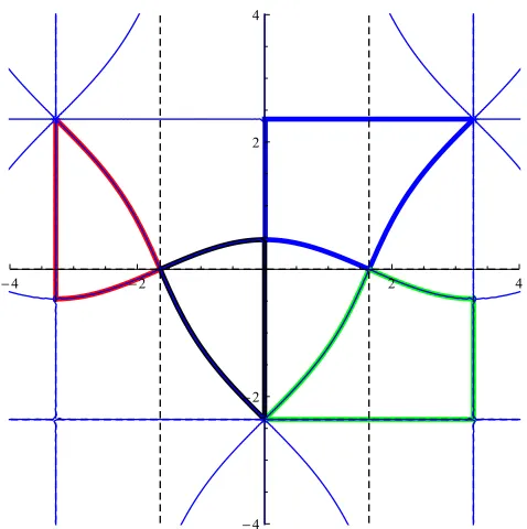
It seems advantageous to consider α ∈ _C as the independent parameter and therefore Ω as a doubly periodic function of α as in (4.3). There should exist four values of α, which correspond to one value of Ω. To be more precise, for the physical spectrum we are looking for all values ofα, which correspond to areal Ω2. The analysis of AppendixB.1is devoted to this study, and is nicely summarized in Fig. 1 where in the complex α plane the lines where Ω2(α) is real are plotted. The “physical” four linear independent solutions of the fourth order differential operator (2.15) live on these lines, and in the fundamental domain represented in Fig. 2 they correspond to the different colours. In the following let 0< k <1/√2. The case 1/√2 < k < 1 can be obtained by applying the duality transformation of Appendix B.2 on the following results.

For a given real value of Ω2 the four independent solutions read

fi(x,Ω, k) =

H(x+αi)

Θ(x) e

−x[Z(αi)−ikcn(αi)]_{, i= 1, . . . ,4, (4.4)}

where the αi as function of Ω have to be chosen according to the range of Ω. For example,

for−∞<Ω2<0, one has

α1(Ω, k) = u(Ω, k)−iv(Ω, k), (4.5)

α2(Ω, k) = 2K−u(Ω, k) +iv(Ω, k),

α3(Ω, k) = 2K+u(Ω, k) +iv(Ω, k),

α4(Ω, k) = 2K−u(Ω, k) + 2iK0−iv(Ω, k), where

u(Ω, k) = sn−1hq_Ω22(1−

√

1−Ω2_{), k}i_{, v(Ω, k) = sn}−1hqΩ2_−2k2_+2k2√_1−Ω2

Ω2_−4k2_k02 , k

-5 0 5 -5

[image:20.612.180.409.82.316.2]

0 5

Figure 1: In the complexα plane one can plot the lines where Ω2(α) is real. The “physical” four linear independent solution live on these lines. The green dots represent places where Ω2= 0, red for Ω2 = 4k2k02, blue for Ω2 = 1 and black for poles. We have chosenk= 0.4.

-4 -2 2 4

-4 -2 2 4

[image:20.612.174.413.413.653.2]

The expressions for the αi’s in the other ranges of Ω are collected in (B.25)-(B.30). The

quasi-momenta pi are obtained by fi(x+ 2K) =e2Kipifi(x) as

pi(Ω, k) =iZ(αi, k) +kcn(αi, k)−

π

2K, (4.7)

where the corresponding αi(Ω, k) have to be chosen according to the previous list. By

construction23, only two of the quasi-momenta are independent, which we will callp1 andp2.

Theexact determinant of the Landau-Lifshitz model defined by (2.11)-(2.19), using (3.16) with 2L= 4K, reads then

detOLL = 16 sin2 2Kp1(Ω, k)

sin2 2Kp2(Ω, k)

. (4.8)

We can immediately recover the characteristic frequencies of the problem, found in [24] using operator methods up to second-order perturbation theory, by simply looking at the zeroes of the determinant (4.8), where the quasi momenta are built with theα’s in the branch Ω2 > 0 and are Taylor-expanded around k = 0. It is enough to look to the factor in (4.8) involvingp1, whose expansion re-expressed in terms of the ω is

p1 =√2ω+ 1− ω 2√2ω+ 1k

2₊ −10ω4−11ω3+ 6ω+ 2

32ω2_{(2ω+ 1)}3/2 k 4

+ −22ω

7_−39ω6_−19ω5_{+ 2ω}4_{+ 10ω}3_{+ 16ω}2_{+ 10ω+ 2}

64ω4_{(2ω+ 1)}5/2 k

6_+O(k8_{). (4.9)}

Inserting it into (4.8) and requiring the vanishing of the expression order by order in small k2, one finds the (squared) frequencies to be

ω2= 1 4(n

2₋₁₎2₊1 4(1−n

2_)k2₊ 3n

4_−2n2_{+ 15}

64(1−n2₎ k 4₋ n

8_+n6_{+ 7n}4_{+ 27n}2_{+ 28}

128 (n2₋₁₎3 k

6_{+O k}8

,

(4.10) where we do not report higher orders, but notice that it is straightforward to calculate them. The first three orders of the expansion above coincide with the ones of [24].

The one-loop correction to theSU(2) LL string energy can be of course obtained perturba-tively via a regularized sum over the frequencies given above [24], or exactly in terms of the one-loop world-sheet effective action Γ(1), and thus in terms of the corresponding partition functionZLL, as follows

E1 = Γ (1) T =−

logZLL

T , T =

Z ∞

−∞

dτ . (4.11)

The Euclidean LL partition function is obtained from the functional determinant as

ZLL = det−1/2OLL, (4.12)

which using (4.8) can be explicitly written as 24

Γ(1)=−logZLL =

T 2

Z ∞

−∞

dΩ 2π log

16 sin2 2Kp1(Ω, k)

sin2 2Kp2(Ω, k)

. (4.13)

23

See discussion around (3.12)-(3.13).

Above, the Euclidean setting requires the quasi-momentapi to be built out of theα’s in the

branch Ω2_{<0, which are given in (4.5). The integral in (4.13) is divergent. A first meaningful} choice of regularization of the functional determinant is to refer it to the k= 0 case. Indeed this limit, as discussed in [24], represent a nearly point-like string and the correction to the ground-state energy should vanish. Hence, we obtain

Γ(1)_reg= T 2

Z ∞

−∞

dΩ 2π log

"

sin2 2Kp1(Ω, k)

sin2 2Kp2(Ω, k)

sin2 π p1(Ω,0)

sin2 π p2(Ω,0)

#

(4.14)

where, at the denominator, the quasi-momenta pi(Ω,0) are computed at k= 0. In order to

analytically perform the above integral over Ω, we can resort to the short string expansion k2 '0. This again means to consider the smallkexpansion of quasi-momentapi(which differ

from the ones considered above, as we are in a different branch for the α’s), as reported in Appendix B.4, and then after, to integrate over Ω the corresponding expressions computed order by order ink. Each term in thek2-series for Γ(1)regmust be further regularized, which is of

course expected as only certain bosonic degrees of freedom and no fermionic ones (crucial for UV finiteness) participate to the effective LL action. In AppendixB.4we report two different ways of regularizing (one inspired byζ-function regularization and one with standard cutoff) which lead to the same result. The resulting expression for the k2-expansion of the one-loop energy is the same as in [24]

E1 = Γ(1)reg

T = 1 4k

2₊ 1

16

1−π 2 3

k4+O(k5). (4.15)

It is interesting to notice that this result follows smoothly by our standard regularization of the 2d LL string effective action, while in [24] it is implied by a ζ-function regularization supplemented by a general prescription for the vacuum energy in terms of characteristic frequencies of a mixed system of oscillators [37].

From equation (2.7), in terms of the physical parameterJ2/J, the short string limitk2→0 reads

J2

J =

k2 2 +

k4

16+O(k

5_{), k}2₌ 2J2

J −

1 2

J2 J

2

, (4.16)

and the expression for the energy becomes

E1 = ˜ λ 2

J2 J +

1 4 −

π2 6

J2 J

2!

+O

J2 J

2!

, (4.17)

where we restored the ˜λ dependence. The first three terms in the formula above are in agreement with [24].

For completeness, we mention that the analysis for the LL folded string in the SL(2) sector (where strings rotate in AdS3 ⊂AdS5 with center of mass moving along a big circle of S5) is totally analogous. Using the following analytical continuation [24,32]

one can easily see that the system of coupled fluctuations is effectively described by the fourth order differential operator in (2.20) where nowk2 _{is negative. Its solutions are then trivially} generalised to the case k2 <0 as basically in each formula one should substitute k→ √−k2 and omit all imaginary constantsiin the exponentials.

4.2 Folded string in full bosonic sigma-model

The fourth order differential operator in (2.39) 25 is again of the type (3.17) with the identi-fication

α0 = 2( ¯Ω2+k2+ 1), α1=−8, β0 =β1= 0, β2 =−4

γ0 = [(−Ω¯2+ 1 +k2)2−4k2]− 4ν 2_Ω¯2 ¯

w2_−ν2, γ1 =γ2=γ3 = 0, (4.19) where ¯Ω is defined in (2.40). Using the consistency equations (3.34) one finds

λ=±

q

k2_sn2_(α)−Ω¯2 _{, (4.20)}

where the relation between ¯Ω andα is

8k4sn4(α)−4(1+k2+ ¯Ω2)k2sn2(α)±8k2sn(α)cn(α)dn(α)pk2_sn2_(α)−Ω¯2₋4ν2_Ω¯2

¯

w2_−ν2 = 0. (4.21)

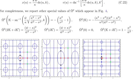
The study reported in AppendixC.2shows that the “physical” four linear independent solu-tions of (2.39) live on the straight and ellipse-like lines in Fig. 3.

Using infi(x+ 2K) =e2Kipifi(x) their explicit expressions - cf. (C.24) - the quasi-momenta

are then obtained as

pn( ¯Ω) =±i

Z(αn) +

ksn(αn)

(κ2_−ν2_)sn2_(α

n) +ν2

κw¯±pκ2_−ν2p_w¯2_−ν2_cn(α

n)dn(αn)

+ π 2K, (4.22) where αn as function of ¯Ω has to be chosen from the list in (C.26)-(C.34). The functional

determinant is again given by

detOν = 16 sin2(L p1) sin2(L p2) , (4.23)

with 2L= 4K.

As a first check of the correctness of the procedure, one can take the long string limit k→1, w¯2→κ2 (see SectionC.1) and look at the zeroes of the expression above choosing the positive-frequency range (C.32) and (C.34) for theα’s in (4.22). We obtain the characteristic frequencies 26

ωn=

q

n2_{+ 2κ}2_±2p_κ4_+n2_ν2_{, (4.25)}

25_{In this section we are working in Minkowski signature, so that (4.19) are obtained from (3.17) analytically} continuing the frequencies.

26

In this limit, we obtain, from (C.32) and (C.34),

sn(α1,2)→ −ν2ω/

hp

κ2_−ν2

r

κ2_±p

-4 -2 2 4 ReHΑL

[image:24.612.193.390.72.261.2]

-4 -2 2 4 ImHΑL

Figure 3: The places, in the fundamental domain of the complex α plane, where the four linear independent solutions (C.24)-(C.25) (marked with different colours) for the fourth order differential operator (2.39) live. Here we have chosenk= 3, w= 6, ν = 2.5. See also Fig. 4.

which is the same result as found in [5]27, see also (C.12).

Since we are missing (see Introduction and Section 2.2.2) the fermionic counterpart of (4.23), we cannot proceed with the exact evaluation of the full (superstring) one-loop partition function on the folded two-spin solution. However, we observe that a nice consequence of our procedure is the possibility of making a non-trivial, analytical statement on the equivalence of partition functions in conformal and static gauge in the single-spin (ν = 0) case. While here the fermionic determinant can be given exactly for all values of the spin [17], it is only the bosonic partition function in static gauge where fluctuations are naturally decoupled -which has been written down in an analytically exact closed form, and reads [17]

logZ_{static gauge}bos =− T 2

Z

dω 2π log

detO_φdet2O_βdet5O0

(4.27)

where

detOφ= 4 sinh2[2 ˜KZ(αφ|k˜2)], detOβ = 4 sinh2

2KZ(αβ|k2)

, detO0 = 4 sinh2(πω) (4.28)

and

sn(αφ|k˜2) =

1 ˜ k

s

1 +

πω 2 ˜K

2

, sn(αβ|k2) =

1 k

r

1 +k2₊πω 2K

2

, (4.29)

with ˜k2 = 4k/(1 +k)2 and ˜K = K(˜k2). The analysis in Section 2.2.1 shows that, in con-formal gauge, the spectral problem associated to the mixed-mode, 3×3 matrix differential

27

One can obtain this result also from (2.39), which in this limit becomes

lim k→1O

(4)

=∂x4+ 2[ω 2

−2(κ2−ν2)]∂2x+ (ω 4

operator corresponding to (2.28)-(2.30) can be evaluated, see (2.38), via the product of a free determinant times the determinant of the fourth order differential operator (2.39), and thus28

logZ_{conformal gauge}bos =−T 2

Z

dω 2π log

detOν=0det2Oβdet4O0

, (4.30)

where in the counting of massless operators we already have taken into account the two conformal gauge massless ghosts [38], and (see AppendixC.3)

detOν=0 = 16 sinh2

2K

Z(α|k2) +1 + cn(α|k

2_)dn(α|k2₎ sn(α|k2₎

sinh2(2KΩ)¯ , (4.31)

with (switching to Euclidean signature)

sn2(α|k2) = −4 ¯Ω 2

(1 +k2_−Ω¯2₎2_−4k2 . (4.32)

One can see that the second factor in (4.31) corresponds to the same massless boson mode of (4.28) (recalling (2.40) and that for ν = 0 it is ¯w= 2K

π ), while for the first factor one should

use for the Jacobi Zeta function the transformation (C.35) which, writing ˜α =α/(1 + ˜k0) + iK0/(1 + ˜k0), leads to the identity

2K

Z(α|k2) +1 + cn(α|k

2_)dn(α|k2₎ sn(α|k2₎

= 2 ˜KZ( ˜α|˜k2) +iπ . (4.33)

This establishes analytically the equivalence of static and conformal gauge bosonic determi-nants (4.27)-(4.30) 29_.

5

Outlook

In this paper we have made a first step into the analytic solution of the matrix fluctuations de-terminant for nontrivial string configurations relevant for the study of the AdS/CFT integrable systems, evaluating exactly the one-loop partition function for the quantum Landau-Lifshitz model on the SU(2) folded string solution of [24]. The same procedure allows the diagonal-ization of the bosonic sector of fluctuations of the full AdS5×S5 excitations over the two-spin folded string solution of [16].

28

While we worked at the operatorial level with the linearized (near folded string solution) form of the string equations of motion, and did not prove the formal equivalence between the determinant of the 3×3 matrix differential operator corresponding to (2.28)-(2.30) and the product detOν=0detO0, (4.30) should be formally correct. This is not different from the steps (2.11)-(2.19) followed in setting the LL spectral problem, with a new ingredient here consisting in the implementation of Virasoro constraints. As thoroughly discussed in [17], at the level of path integral the step analogous to (2.33)-(2.34) will produce an extra detO0 factor as required for balance of degrees of freedom.

29

At the operator level, it was noticed already in [17] that Oν=0 manifestly factorizes as a product of two second-order ones

Oν(4)=0=O1· O2, O1= (ρ

0

)−1h∂σ2+ω2−2ρ

02₋

2κ 2_w2

ρ02

i

ρ0, O2=ρ

0

[∂σ2+ω2] (ρ

0

This result calls for the complete (i.e. including fermions) solution of the fluctuation prob-lem for non-homogeneous configurations of elliptic type, which might require a nontrivial field redefinition for the corresponding Lagrangian, or equivalently a modification of the ansatz for the solution of the related differential operator. This class of solutions includes the relevant case of open string configurations corresponding to the space-like Wilson loops of [22] (also in other backgrounds [23]). Completing in this sense the analysis here performed should give an answer to the caveats of the semiclassical analysis mentioned in the Introduction, enlarging the range of applicability of the procedure and opening the way to the detailed understanding of the relation between this quantum field-theoretical approach and the one based on the algebraic curve [39].

Acknowledgments

We are grateful to M. Beccaria, G. Dunne and A. A. Tseytlin for earlier collaboration on the topic of Section 2.2.1and C.1. It is a pleasure to thank M. Beccaria, G. Dunne, S. Frolov, L. Griguolo, D. Seminara, L. Thorlacius and A. A. Tseytlin for discussions. The work of V.F., M.P. and E.V. is funded by the Emmy Noether Programme “Gauge Field from Strings” funded by DFG. M.P. also acknowledges support from SFB 647 ”Space-Time-Matter. Analytic and Geometric Structures”. V.G.M.P. acknowledges partial support from Swedish Research Council for funding under the contract 623-2011-1186.

A

The squared Lam´

e operator

As a check of the procedure described in Section3and of the involved algebraic manipulations there performed, we consider the fourth order differential operator obtained by squaring the Lam´e operator

O_L=−∂_x2+ 2k2sn2(x|k2) + Ω2, (A.1)

which gives

O2_L = ∂_x4−2(2k2sn2(x) + Ω2)∂_x2−8k2sn(x)cn(x)dn(x)∂x (A.2)

−8k4sn4(x) + 4(2(1 +k2) + Ω2)k2sn2(x)−4k2+ Ω4 .

Since the solution of the Lam´e equation is well known we can immediately write down the Floquet solutions for

O2

Lf(x) = Λf(x), (A.3)

given by

f1(x) = H(x+α+)

Θ(x) e

−xZ(α+)_{, f2(x) =} H(x−α+)

Θ(x) e

xZ(α+)_{, (A.4)}

f3(x) = H(x+α−)

Θ(x) e

−xZ(α−)_{, f4(x) =} H(x−α−)

Θ(x) e

with

sn(α±|k2) =

s

1 +k2_∓√_{Λ + Ω}2

k2 . (A.5)

For the squared Lam´e operator (A.2) we can read off the coefficients

α0 = −2Ω2, α1 =−4, β0 = 0, β1 = 0, β2=−4 (A.6)

γ0 = − 4 3k

2_{+ Ω}4_{, γ}

1 =

8 3(1 +k

2_{) + 4Ω}2_{, γ}

2 = 0, γ3 =−

4 3.

One can see that the first consistency condition in (3.34) is satisfied. Further one findsλ= 0, which is also consistent with (3.33). Equation (3.32) gives now the relation between Λ and α

k4sn4(α)−2[(1 +k2) + Ω2]k2sn2(α) + (1 +k2+ Ω2)2 = Λ, (A.7)

which can be solved as

sn(α±|k2) =

s

1 +k2_∓√_{Λ + Ω}2

k2 , (A.8)

which agrees with the result (A.5) directly obtained using the square property.

B

Landau-Lifshitz

SU

(2) folded string analysis: details

B.1 Spectral domain

Useful properties of Ω± defined in (4.3) are

Ω±(−α, k) = −Ω∓(α, k),

Ω±(α+ 2iK0, k) = −Ω∓(α, k),

Ω±(α+K+iK0, k) = ∓Ω∓(iα, k0),

Ω±(α+ 2K+ 2iK0, k) = −Ω±(α, k) . (B.1)

It is then easy to see that Ω±(α) is a doubly periodic function

Ω±(α+ 4K, k) = Ω±(α, k), Ω±(α+ 4iK0, k) = Ω±(α, k) (B.2)

Important special values are

Ω2₊(K, k) = 0, Ω2+(iK

0

, k) = 1,

Ω2₊

iK0+icn−1

k2 k02 , k

0

, k

= Ω2₊

iK0−icn−1

k2 k02, k

0

= 4k2k02. (B.3)

For the physical spectrum only those values of the complex parameterα =u+ivcorresponding to a real Ω2 are of interest. We decompose

with

Re(Ω+)(u, v) = 2kdn(u, k)(dn(v, k

0_{)−kcn(u, k)sn(v, k}0₎₎

(1−dn2(u, k)sn2_{(v, k}0₎₎2 (cn(u, k)cn 2_{(v, k}0

) +ksn2(u, k)sn(v, k0)dn(v, k0)),

Im(Ω+)(u, v) = 2ksn(u, k)cn(v, k

0_{)(dn(v, k}0_{)−kcn(u, k)sn(v, k}0₎₎

(1−dn2(u, k)sn2_{(v, k}0₎₎2 (kcn(u, k)−dn

2_{(u, k)sn(v, k}0

)dn(v, k0)).

In order to have Ω2₊ real, we find the cases

• v=K0, then

Ω+(u+iK0) = 2dn(u, k)

sn2_{(u, k)}(1−cn(u, k)). (B.5)

Settingu= 2wgives

Ω+(2w+iK0) = dc2(w, k)−k2sn2(w, k). (B.6) Varyingwfrom 0 to K, then Ω2+(2w+iK0) covers the interval [1,∞). Therefore we can solve forw as

sn2(w) = 1− Ω 2k2 +

1 2k2

p

Ω2_−4k2_k02_{, (B.7)}

with

0<sn2(w)<1 for 1<Ω<∞. (B.8)

• u= 0, then

Ω+(iv) = 2k

cn2_{(v, k}0₎(dn(v, k

0_{)−ksn(v, k}0_{)). (B.9)}

Varying v from K0 −cn−1(k2/k02, k0) to K0, then Ω2+(iv) covers the interval [4k2k02,1]. Therefore we can solve forv as

sn2(v, k0) = 1 +4k 2 Ω2

h

−1 + 2k2+pΩ2_−4k2_k02i_{, (B.10)} with

k2 k02 <sn

2_{(v, k}0_{)<1 for 2kk}0 _{<Ω<1 and 0< k}2 _< 1

2. (B.11)

• kcn(u, k)−dn2(u, k)sn(v, k0)dn(v, k0) = 0

For 0< u <K this can be solved forv=v(u, k) as

sn2(v, k0) = 1−

r

1−4k2_k02 cd2(u,k) dn2_(u,k)

2k02 , (B.12)

then

α(u, k) =u+isn−1



 

1 √

2k0

v u u

t1−

s

1−4k2_k02cd 2_{(u, k)} dn2(u, k), k

0





. (B.13)

After using some elliptic function identities one finds

Ω2₊(α(u, k), k) = 4k2k02cn 2_{(u, k)}

Solving for u gives

sn2(u, k) = 1 k2 +

2k02 k2

√

1−Ω2₋₁

Ω2 , (B.15)

with

0<sn2(u, k)<1, for 0<Ω<2kk0 and 0< k2 < 1

2. (B.16)

• cn(u, k)cn2(v, k0) +ksn2(u, k)sn(v, k0)dn(v, k0) = 0 ForK< u <2Kthis can be solved for v as

sn2(v, k0) = 2cn

2_{(u, k)} 2cn2_{(u, k) +k}2_sn4_{(u, k) +k}2_sn2_(u)p

4cn2_{(u, k) + sn}4_{(u, k)} =

= 2cn

2_{(u, k) +k}2_sn4_{(u, k)−k}2_sn2_{(u, k)}p

4cn2_{(u, k) + sn}4_{(u, k)} 2(cn2_{(u, k) +k}2_k02_sn4_{(u, k))} =

=

2_sncn24₍(_u,ku,k)₎ +k2−k2

q

1 + 4cn_sn42(₍u,k_u,k))

2

k2_k02₊ cn2(u,k) sn4_(u,k)

, (B.17)

and then

α(u, k) =u+isn−1



 

v u u u t

2_sncn42₍(_u,ku,k₎)+k2−k2

q

1 + 4cn_sn24(₍u,k_u,k))

2

k2_k02₊cn2(u,k) sn4_(u,k)

, k

0





. (B.18)

After using some elliptic function identities one finds

Ω2₊(α(u), k) =−4cn 2_{(u, k)}

sn4_{(u, k)} , for K< u <2K, (B.19) or

Ω2₊(α(˜u+K), k) =−4k02sn

2_{(˜u, k)dn}2_{(˜u, k)}

cn4_{(˜u, k)} . (B.20)

Solving for u gives

sn2(u, k) = 2 Ω2(1−

p

1−Ω2_{), (B.21)}

with

0<sn2(u, k)<1 for − ∞<Ω2 <0. (B.22)

The expressions of αi’s in the different branches for Ω2 read as follows:

• For−∞<Ω2 <0 as

α1(Ω, k) = u(Ω, k)−iv(Ω, k),

α2(Ω, k) = 2K−u(Ω, k) +iv(Ω, k),

α3(Ω, k) = 2K+u(Ω, k) +iv(Ω, k),

where

u(Ω, k) = sn−1

"r

2 Ω2(1−

p

1−Ω2_{), k}

#

, v(Ω, k) = sn−1



 s

Ω2_−2k2_{+ 2k}2√_1−Ω2 Ω2_−4k2_k02 , k

0



 .

(B.24)

• For 0<Ω2 <4k2k02 as

α1(Ω, k) = 2K−u2(Ω, k)−iv2(Ω, k), α2(Ω, k) = u2(Ω, k) +iv2(Ω, k), α3(Ω, k) = 2K+u2(Ω, k)−iv2(Ω, k),

α4(Ω, k) = 2K−u2(Ω, k) + 2iK0+iv2(Ω, k), (B.25) where

u2(Ω, k) = sn−1





1 k

s

1−2k021− √

1−Ω2 Ω2



, v2(Ω, k) = sn−1

1 √

2k0

q

1−p1−Ω2_{, k}0

.

(B.26)

• For 4k2k02 <Ω2<∞ as

α3(Ω, k) = 2K−iK0+ 2iα0(Ω, k0),

α4(Ω, k) = 2K+ 3iK0−2iα0(Ω, k0). (B.27) • For 4k2k02 <Ω2<1

α1(Ω, k) = 2K−isn−1

"r

1−4k 2 Ω2

1−2k2₋p_Ω2_−4k2_k02_{, k}0

#

,

α2(Ω, k) = isn−1

"r

1−4k2 Ω2

1−2k2₋p_Ω2_−4k2_k02_{, k}0

#

. (B.28)

• For 1<Ω2 _{<∞ as}

α1(Ω, k) = 2K−iK0−2α0(Ω, k)

α2(Ω, k) = iK0+ 2α0(Ω, k), (B.29)

where

α0(Ω, k) = sn−1

"r

1− Ω 2k2 +

1 2k2

p

Ω2_−4k2_k02_{, k}

#

. (B.30)

B.2 A duality property of the LL fourth order differential operator

Definingz=ix we can rewrite (2.20) as

O(4)_{(z, k}0_)f

1,2(−iz−K+iK0, α, k) = Ω−2(α, k)f1,2(−iz−K+iK0, α, k),