Spatial exporters

      

City, University of London Institutional Repository

Citation

:

Defever, F., Heid, B. and Larch, M. (2015). Spatial exporters. Journal of

International Economics, 95(1), pp. 145-156. doi: 10.1016/j.jinteco.2014.11.006

This is the supplemental version of the paper.

This version of the publication may differ from the final published

version.

Permanent repository link:

http://openaccess.city.ac.uk/16008/

Link to published version

:

http://dx.doi.org/10.1016/j.jinteco.2014.11.006

Copyright and reuse:

City Research Online aims to make research

outputs of City, University of London available to a wider audience.

Copyright and Moral Rights remain with the author(s) and/or copyright

holders. URLs from City Research Online may be freely distributed and

linked to.

City Research Online:

http://openaccess.city.ac.uk/

[email protected]

Online Appendix for

“Spatial Exporters”

Fabrice Defever

∗

, Benedikt Heid

†

, Mario Larch

‡

Forthcoming at the

Journal of International Economics

Abstract

This document presents supplemental material for the paper

“Spatial Exporters”. It contains further descriptive evidence for

firm-specific heterogeneity in export destinations, detailed first stage

re-gression results, further dynamic panel estimates using only a

one-period lag, an additional external instrument as well as results using

the difference-GMM estimator by Arellano and Bond (1991), further

multi-product firm regressions, miscellaneous robustness checks, all

re-gressions from the main text including country-specific time trends,

dynamic panel results for a sample including firms which entered

MFA-restricted countries between 2000 and 2004, as well as the empirical

probabilities of exporting to a country and descriptive statistics of the

samples used in the main text.

∗

_{University of Nottingham, GEP and CEP/LSE,}

_{[email protected]}

†

_{University of Bayreuth,}

_{[email protected]}

‡

_University

_of

_Bayreuth,

_ifo

_Institute,

_CESifo

_and

_GEP,

Appendix

A

Evidence for firm-specific heterogeneity in

export destinations

In order to shed light on the entry of firms into different markets in our sample

of firms, we follow Eaton et al. (2011) and first assume that firms follow a

common hierarchy, meaning that a firm that sells to the

k

+ 1st most popular

export destination necessarily sells to the

k

th most popular destinations as

well. We present the top seven export destinations of the Chinese exporters in

our sample, excluding the MFA-restricted countries. In Table A.1 we report

the number of firms exporting to each of the seven most popular destinations,

as well as the unconditional empirical probability of Chinese exporters selling

there. We clearly see that common gravity variables, like distance and country

size, matter.

Again following Eaton et al. (2011), in Table A.2 we report strings of the

top-seven destinations that obey a hierarchical structure, alongside the

num-ber of firms selling to each string. For example, the export string JPN means

that the firm exports to Japan but to no other destination among the top 7

non-MFA destinations. Similarly, the string JPN-KOR means that the firm

exports to Japan and South Korea but no other destination among the top

7 non-MFA destinations, and so forth. Overall, 66 percent (861/1295) of all

firms in our sample adhere to the hierarchy given by the top seven non-MFA

export destinations. Hence, about a third of the firms export to a different

set of countries, implying a substantial amount of heterogeneity across firms

in terms of the set of export destinations they serve. The column labeled

“In-dependence” in Table A.2 reports, based on the unconditional probabilities

presented in Table A.1, the number of firms selling to each hierarchical string

assuming independence across destination choices of a firm. If a firm chose

export destinations independently, the number of firms sticking to the

[image:4.612.170.444.157.326.2]

Table A.1: Chinese Textile and Apparel Firms

Export-ing to the Seven Most Popular Non-MFA Destinations

in 2006

Export destination

Number of

exporters

Fraction of

exporters

Japan (JPN)

973

0.751

South Korea (KOR)

328

0.253

Singapore (SGP)

81

0.063

Australia (AUS)

70

0.054

Vietnam (VNM)

62

0.048

Thailand (THA)

57

0.044

Malaysia (MYS)

46

0.036

All Chinese exporters

∗

1,295

Notes:∗in our sample. Table shows the seven most popular export desti-nations of the 1,295 textile and apparel firms in our sample excluding the 27 MFA/ATC restricted export destinations for the year 2006. The table follows closely Table I in Eaton et al. (2011). We describe the construction of the sample in detail in Section 2.1 of the main manuscript.

the common hierarchy, i.e. 12 percent more than what independence would

imply. Hence, in our empirical specification we will have to take into account

that export destinations within firms are clustered spatially, and that there is

considerable heterogeneity in export destinations across firms. We therefore

[image:5.612.140.473.301.463.2]

Table A.2:

Chinese Textile and Apparel Firms Exporting to

Strings of Top-Seven Non-MFA Destinations in 2006

Number of Exporters

Export String

a

_Data

_Independence

JPN

676

565

JPN-KOR

175

191

JPN-KOR-SGP

8

13

JPN-KOR-SGP-AUS

1

1

JPN-KOR-SGP-AUS-VNM

0

0

JPN-KOR-SGP-AUS-VNM-THA

0

0

JPN-KOR-SGP-AUS-VNM-THA-MYS

1

0

Total

861

770

Notes:a_{The export string JPN means exporting to Japan but no other destination among}

B

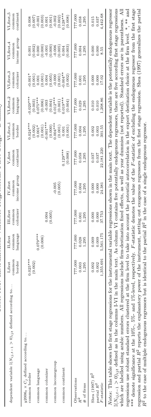
Detailed first stage regression results

We present detailed results of the first stage regressions for the instrumental

panel regressions presented in Section 3.3 in the main manuscript in Tables

A.3 and A.4.

Weak instrument test statistics are derived under the assumption of

iid

errors. If errors are not

iid

, Baum et al. (2007) propose to still use these

statistics and compare them to the Stock and Yogo (2005) critical values or

the Staiger and Stock (1997) rule of thumb of a

F

-statistic for the excluded

instruments in the first stage regression to be larger than 10. In our case, all

the tests reject that we have a weak instrument problem.

We also provide the partial

R

2

_{(i.e. the}

_R

2

_{of the instrument in the first}

stage regression, netting out the explanatory power of exogenous regressors).

It measures the explanatory power of our instruments.

Admittedly, these

are very low. However, this has to be put in perspective: We use a discrete

choice panel of export decisions at the firm level.

R

2

measures of demeaned

panel models such as ours (i.e. of within-models which remove the explanatory

power of the firm-destination fixed effects) for firm-level studies tend to be low,

even more so for discrete choice data sets of export destination choices, see

Albornoz et al. (2012). Therefore, even though low partial

R

2

_{s are not exactly}

good news, we would like to stress that a low partial

R

2

_{is only a problem if we}

had weak instruments which are not strictly exogenous. If one believes in our

instruments, then we get consistent estimates even if the explanatory power

of the instrument is weak. Also, please note that our instruments only vary at

the country level by construction; actually, this is the motivation behind our

[image:7.612.190.439.14.701.2]

C

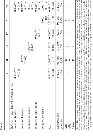
Dynamic Panel Estimates Using Only

One-Period Lag with Country-Specific Time Trends

In Tables A.5 and A.6 we present results for System-GMM estimates of the

dynamic panel model using only one lag. As can be seen, while coefficient

estimates remain similar to our preferred specification, the specifications with

[image:10.612.113.504.122.705.2]

D

Dynamic Panel Estimates Using an

Addi-tional External Instrument

Dynamic panel models have been developed to provide consistent parameter

estimates when only internal instruments are available. However, they also

allow to include external instruments to receive additional moment conditions

for estimation. We present results where we include our proposed instruments

(

y

2006

t

×

C

j

and

y

2006

t

×

N

j

, respectively) from the instrumental variable

regressions from Section 3.3 in the main manuscript in Tables A.7 and A.8.

Qualitatively, results remain similar, but model specification tests perform

considerably better, as the Sargan test for the validity of our instruments

cannot be rejected for the majority of specifications in Table A.7. This provides

E

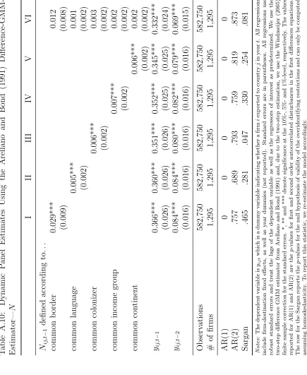
Dynamic Panel Estimates Using the

Arel-lano and Bond (1991) Difference-GMM-Estimator

In Tables A.9 and A.10 we use the Difference-GMM estimator from Arellano

and Bond (1991) instead of the System-GMM estimator from Blundell and

Bond (1998) used in the main manuscript. The Difference-GMM estimator

has the main advantage of being more robust in the sense that less restrictive

moment conditions are used for estimation. However, it may suffer from severe

finite sample bias if the persistence of the dependent variable is high. Note

that using the Difference-GMM estimator we lose an additional year of our

dataset for the estimation. Results stay very similar. In addition, the model

specification tests perform considerably better compared to the System-GMM

estimates as they do not reject the model in the majority of cases, including

[image:16.612.92.516.123.684.2]

[image:17.612.87.522.145.676.2]

F

Multi-Product Firms: Dynamic Panel Estimates—

N

In Table A.11 we present multi-product regressions with the number of

con-tiguous export destinations as an alternative regressor:

y

ijt

=

φ

1

y

ij,t−1

+

φ

2

y

ij,t−2

+

δ

1

N

ij,tsameproduct−1

+

δ

2

N

ij,totherproducts−1

+

θ

ij

+

θ

t

+

ijt

.

(1)

By and large, results are very similar when compared to Table 8 in the main

text. Common border for the same product has again the largest marginal

effect. We again do not find evidence for across product learning. Interestingly,

we now find a small but positive and significant effect of having exported to a

G

Miscellaneous robustness checks

Table A.12 presents the regression results for the first six robustness checks

discussed in Section 5 in the main manuscript concerning lagged export values,

competitors’ success, trading agents, state-owned firms, foreign-owned firms,

and processing trade.

In Table A.13, we present results for the diff-in-diff specification excluding

T

able

A.13:

Diff-in-Diff

Excluding

Russia

I

II

II

I

IV

V

VI

y

2006

t

×

C

j

defined

according

to.

..

common

b

order

0.001***

0.001***

(0.000)

(0.000)

common

language

0.000

0.000

(0.000)

(0.000)

common

colonizer

-0.000

-0.000

(0.000)

(0.000)

common

income

group

-0.000

-0.000*

(0.000)

(0.000)

common

con

tinen

t

0.000***

0.000

(0.000)

(0.000)

Observ

ations

771,820

771,820

771,820

771,820

771,820

771,820

#

of

firms

1,295

1,295

1,295

1,295

1,295

1,295

Notes

:

The

dep

enden

t

v

ariable

is

yij

t

whic

h

is

a

dumm

y

v

ariable

indicating

whether

a

firm

i

exp

o

rted

to

coun

try

j

in

y

ear

t

.

All

regressions

include

firm-destination

fixed

e

ffects,

as

w

ell

as

y

ear

dummies

(not

rep

orted).

Standard

error

s

are

in

paren

theses.

All

regressions

use

robust

standar

d

errors

clustered

at

the

coun

try

lev

el

to

tak

e

in

to

accoun

t

that

the

regressor

only

v

aries

at

the

coun

try

lev

el

follo

wing

the

suggestion

for

diffe

re

nces-in-differences

estimates

b

y

Bertrand

et

al.

(2004).

*,

**

and

***

denote

significance

at

the

10%-,

5%-and

1%-lev

el,

resp

ectiv

ely

[image:22.612.167.443.141.674.2]

H

Controlling for country-specific time trends

Tables A.14 to A.30 present all the tables from the main manuscript including

country-specific time trends as discussed in Section 5 in the main manuscript

under the heading “

Country-specific time trends

”.

H.1

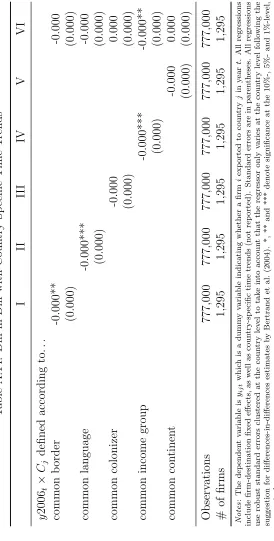
Diff-in-Diff

Table A.14 reports the difference in difference estimates. Clearly, we

can-not identify any significant effect of spatial exporters when including

country-specific time trends. This is not too surprising, however, as our treatment only

varies at the country-level and does not use any firm-specific information for

identification.

We therefore also tried out continent-specific time trends. As expected,

results lie in between the estimates without the time trends and the

country-specific time trends. Specifically, sharing a common border remains significant.

T

able

A.14:

Diff-in-Diff

with

Coun

try-Sp

ecific

Time

T

rends

I

II

II

I

IV

V

VI

y

2006

t

×

C

j

defined

according

to.

..

common

b

order

-0.000**

-0.000

(0.000)

(0

.000)

common

language

-0.000***

-0.000

(0.000)

(0.000)

common

colonizer

-0.000

0.000

(0.000)

(0

.000)

common

income

group

-0.000***

-0.000**

(0.000)

(0.000)

common

con

tinen

t

-0.000

0.000

(0.000)

(0.000)

Observ

at

ions

777,000

777,000

777,000

777,0

00

777,000

777,000

#

of

firms

1,295

1,295

1,295

1,295

1,295

1,295

Notes

:

The

dep

enden

t

v

ariable

is

yij

t

whic

h

is

a

dumm

y

v

ariable

indicating

whether

a

firm

i

exp

orted

to

coun

try

j

in

y

ear

t

.

All

regressions

include

firm-destination

fixed

effects,

as

w

ell

as

coun

try-sp

ecific

time

trends

(not

rep

orted).

Standard

errors

are

in

paren

theses.

All

regressions

use

robust

standard

err

ors

clustered

at

the

cou

n

try

lev

el

to

tak

e

in

to

accoun

t

that

the

regressor

only

v

aries

at

the

coun

try

lev

el

follo

wing

the

suggestion

for

differences-in-differences

estimates

b

y

Bertrand

et

al.

(2004).

*,

**

and

**

*

denote

significance

at

the

10%-,

5%-and

1%-lev

el,

resp

e

ctiv

ely

[image:24.612.167.441.132.673.2]

T

able

A.15:

Diff-in-Diff

with

Con

tinen

t-Sp

ecific

Time

T

rends

I

II

II

I

IV

V

VI

y

2006

t

×

C

j

defined

according

to.

..

common

b

order

0.001***

0.001**

(0.000)

(0.00

0)

common

language

-0.000

0.000

(0.000)

(0.000)

common

colonizer

-0.000***

-0.000*

(0.000)

(0.000)

common

income

group

-0.000**

-0.000**

(0.000)

(0.000)

common

con

tinen

t

-0.000

-0.000

(0.000)

(0.000)

Observ

at

ions

7

77,000

777,000

777,000

777,000

777,000

777,000

#

of

firms

1,295

1,295

1,295

1,295

1,295

1,295

Notes

:

The

dep

enden

t

v

ariable

is

yij

t

whic

h

is

a

dumm

y

v

ariable

indicating

whether

a

firm

i

exp

orted

to

coun

try

j

in

y

ear

t

.

All

regressions

include

firm-destination

fixed

effects,

as

w

ell

as

con

tinen

t-sp

ecific

ti

me

trends

(not

rep

orted).

Standard

errors

ar

e

in

paren

the

ses.

All

regressions

use

robust

standard

errors

clustered

at

the

coun

try

lev

el

to

tak

e

in

to

accoun

t

that

the

regressor

only

v

aries

at

the

coun

try

lev

el

follo

wing

the

suggestion

for

differences-in-differences

estimates

b

y

Bertrand

et

a

l.

(2004).

*,

**

and

***

denote

significance

at

the

10%-,

5%-and

1%-lev

el,

resp

ectiv

ely

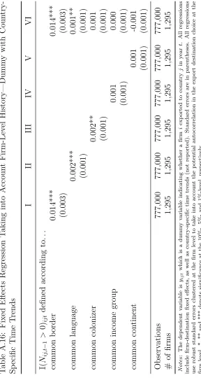
[image:25.612.167.442.136.675.2]

H.2

Fixed effects regression taking into account

firm-level history

Tables A.16 and A.17 present the fixed effects regressions taking into account

firm-level history. In this specifications, results are robust and even become

T

able

A.16:

Fixed

Eff

ects

Regression

T

aking

in

to

Accoun

t

Firm-Lev

el

History—

Dumm

y

with

Coun

try-Sp

ecific

Time

T

rends

I

II

II

I

IV

V

VI

I

(

N

ij

,t

−

1

>

0)

ij

t

defined

according

to.

..

common

b

order

0.014***

0.014***

(0.003)

(0.003)

common

language

0.002***

0.001**

(0.001)

(0.001)

common

colonizer

0.002**

0.001

(0.001)

(0.001)

common

income

group

0.001

0.000

(0.001)

(0.001)

common

con

tinen

t

0.001

-0.001

(0.001)

(0.001)

Observ

ations

777,000

777,000

777,000

777,000

777

,000

777,000

#

of

firms

1,295

1,295

1,295

1,295

1,295

1,295

Notes

:

The

dep

enden

t

v

ariable

is

yij

t

whic

h

is

a

dumm

y

v

ariable

indicating

whether

a

firm

i

exp

o

rted

to

coun

try

j

in

y

ear

t

.

All

regressions

include

firm-d

e

stination

fixed

effects,

as

w

ell

as

coun

try-sp

ecific

time

trends

(not

rep

orted).

Standard

errors

are

in

paren

theses.

Al

l

regressions

use

robust

standard

errors

clustered

at

the

firm

lev

el

to

tak

e

in

to

accoun

t

the

p

oten

tial

auto

correlation

in

the

exp

ort

destination

choice

at

the

firm

lev

el.

*,

**

and

***

denote

significance

at

the

10%-,

5%-and

1

%

-l

ev

el,

resp

ectiv

ely

[image:27.612.159.447.128.681.2]

T

able

A.17:

Fixed

Effects

Regression

T

aking

in

to

Accoun

t

Firm-Lev

el

History—

N

with

Coun

try-Sp

ecific

Time

T

rends

I

II

II

I

IV

V

VI

N

ij

,t

−

1

defined

according

to.

..

common

b

order

0.011***

0.010

***

(0.003)

(0.003)

common

language

0.001**

0.000

(0.001)

(0.000)

common

colonizer

0.003***

0.002**

(0.001)

(0.001)

common

income

group

0.002**

0.001

(0.001)

(0.001)

common

con

tinen

t

0.001

0.00

0

(0.001)

(0.001)

Observ

ations

777,000

777,000

777,000

777,000

777,000

777,0

00

#

of

firms

1,295

1,295

1,295

1,295

1,295

1,295

Notes

:

The

de

p

enden

t

v

ariable

is

yij

t

whic

h

is

a

dumm

y

v

ariable

indicating

whether

a

firm

i

exp

or

te

d

to

c

o

un

try

j

in

y

ear

t

.

All

regressions

include

firm-destination

fixed

effects,

as

w

ell

as

co

un

try-sp

ecific

time

trends

(not

rep

orted).

Standard

errors

are

in

paren

these

s.

All

regressions

use

robust

standard

e

rrors

clustered

at

the

firm

lev

el

to

tak

e

in

to

accoun

t

the

p

oten

tial

auto

correlation

in

the

exp

ort

destination

choice

at

the

firm

lev

el.

*,

**

a

nd

***

denote

significance

at

the

10%-,

5

%-and

1%-lev

el,

re

sp

ectiv

ely

H.3

Instrumental variable regressions

Tables A.18 to A.21 present instrumental variable regressions including

country-specific time trends alongside the accompanying first stage regression results.

Here, results seem not to be robust, with the majority of all estimated

co-efficients being negative and significant. The unrealistically large coefficient

estimates for column III in both Tables A.18 and A.20 hint at very high

mul-ticollinearity between the country-specific time trends and our regressors of

interest. Evidently, identifying coefficients becomes difficult.

We therefore also tried out continent-specific time trends. As expected,

results lie in between the estimates without the time trends and the

country-specific time trends. Specifically, sharing a common border remains significant.

[image:30.612.130.479.130.698.2]

[image:31.612.194.434.36.700.2]

T

able

A.20:

Instrumen

tal

V

ariable

Regressions—

N

with

Coun

try-Sp

ecific

Time

T

rends

I

II

II

I

IV

V

VI

N

ij

,t

−

1

defined

according

to.

..

common

b

order

-0.032

-0.0

11

(0.035)

(0.076

)

common

language

-0.004**

*

0.001

(0.001)

(0.022)

common

colonizer

0.551

0.271

(0.750)

(1.008)

common

income

group

-0.006**

-0.006

(0.003)

(0.007)

common

con

tinen

t

-0.001

-0.001

(0.001)

(0.009)

Observ

ations

777,000

777,000

777,000

777,000

777,000

777,000

#

of

firms

1,295

1,295

1,295

1,295

1

,295

1,29

5

First

stage

F

-statistic

754.3

10,923

0

.316

8,485

5,357

(

)

First

stage

partial

R

2

0.001

0.018

0.000

0.014

0

.009

(

)

Notes

:

The

dep

enden

t

v

ariable

is

yij

t

whic

h

is

a

dumm

y

v

ariable

indicating

whether

a

firm

i

exp

or

te

d

to

coun

try

j

in

y

ear

t

.

All

regressions

include

firm-destination

fixed

effects,

as

w

ell

as

coun

try-sp

eci

fic

time

trends

(not

rep

orted).

W

e

use

the

tw

o-stage

least-squares

within

panel

instrumen

tal

v

ariables

estimator

where

w

e

instrumen

t

the

endogenous

regressor

b

y

y

2006

t

×

Nj

.

Stand

ard

errors

are

in

paren

theses.

All

regressions

use

robust

standard

errors

clustered

at

the

firm

lev

el

to

tak

e

in

to

accoun

t

the

p

oten

tial

auto

correlation

in

the

exp

ort

destination

cho

ice

at

the

firm

lev

el.

*,

**

and

**

*

denote

significance

at

the

10%-,

5%-and

1%-lev

el,

resp

ectiv

ely

.

First

stage

F

-statistic

denotes

the

v

alue

of

the

F

-statistic

of

excluding

the

endogenous

regressor

from

the

fir

st

stage

regression

and

first

stage

par

ti

a

l

R

2

rep

orts

the

explanatory

p

o

w

er

of

the

instrumen

t,

netting

out

exogenous

regressors

from

the

first

stage

regression.

(

):

The

fiv

e

first

stage

regressions

and

statistics

for

the

fiv

e

endogenous

v

ariables

for

column

VI

are

rep

orted

in

T

able

[image:34.612.129.479.134.694.2]

[image:35.612.190.435.35.698.2]

T

able

A.24:

Instrumen

tal

V

ariable

Regressions—

N

with

Con

tinen

t-Sp

ecific

Time

T

rends

I

II

II

I

IV

V

VI

N

ij

,t

−

1

defined

according

to.

..

common

b

order

0.053*

0.074**

*

(0.029)

(0.028)

common

language

-0.001

0.000

(0.001)

(0.00

2)

common

colonizer

-0.060

-0.028

(1.057)

(0.139)

common

income

group

-0.004*

-0.005**

(0.002)

(0.002)

common

con

tinen

t

-0.001

-0.003

(0.001)

(0.002)

Observ

ations

777,000

777,000

777,000

777,000

777,000

777,000

#

of

firms

1,295

1,295

1,295

1,295

1,295

1,295

First

stage

F

-statistic

1,551

19,472

158

.0

15,974

5,358

(

)

First

stage

partial

R

2

0.003

0.032

0.000

0.027

0.009

(

)

Notes

:

The

dep

enden

t

v

a

ri

a

ble

is

yij

t

whic

h

is

a

dumm

y

v

ariable

indicating

whether

a

firm

i

exp

o

rted

to

coun

try

j

in

y

ear

t

.

All

regressions

include

firm-destination

fixed

effects,

as

w

ell

as

con

tinen

t-sp

ecific

time

trends

(not

rep

orted).

W

e

use

the

tw

o-stage

least-squares

within

panel

instrumen

tal

v

ariables

estim

a

tor

where

w

e

instrumen

t

the

endogenous

regressor

b

y

y

2006

t

×

Nj

.

Standard

e

rrors

are

in

paren

theses.

All

regressions

use

robust

standard

errors

clustered

at

the

firm

lev

el

to

tak

e

in

to

accoun

t

the

p

oten

tial

auto

correlation

in

the

exp

ort

destination

choice

at

the

firm

lev

el.

*,

**

and

***

denote

significance

at

the

10%-,

5%-and

1%-lev

el,

resp

ectiv

ely

.

First

stage

F

-statistic

denotes

the

v

alue

of

the

F

-statistic

of

excluding

the

endogenous

regressor

from

the

fir

st

stage

regression

and

first

stage

partial

R

2

rep

o

rts

the

explanatory

p

o

w

er

of

the

instrumen

t,

netting

out

exogenous

regressors

fro

m

the

first

sta

ge

regression.

(

):

The

fiv

e

first

stage

regressions

and

statistics

for

the

fiv

e

endogenous

v

ariables

for

column

VI

are

rep

orted

in

T

able

H.4

Dynamic panel results taking into account state

dependence

Tables A.26 and A.27 present dynamic panel estimates including

country-specific time trends. Results are very similar to the dynamic panel estimates

[image:39.612.109.508.123.696.2]

H.5

Multi-product firms

We present results for multi-product firm regressions including country-specific

time trends in Tables A.28 and A.29. Again, results remain similar to those

[image:42.612.57.562.129.694.2]

H.6

Miscellaneous robustness checks

In this Section, we present the results of including country-specific time trends

I

Different specification for fixed effects

re-gression taking into account firm-level

his-tory

We follow up on footnote 16 in the main manuscript of the paper and

in-troduce

N

_ij,tM F A₋₁

, the number of contiguous previous export destinations which

are MFA countries, and

N

_ij,tnonM F A−1

, the number of contiguous previous

ex-port destinations which are not MFA countries, instead of our default

re-gressor

N

ij,t−1

, the total number of contiguous previous export destinations,

in our regressions from Section 3.2 from the main manuscript which present

fixed effects regressions which take into account firm-level history. Note that

N

ij,t−1

=

N

ij,tM F A−1

+

N

ij,tnonM F A−1

. As always, we begin by presenting results where

we apply

_I

(

N

ij,t−1

>

0)

ijt

to each definition of

N

ij,t−1

. Obviously, evidence for

spatial exporters in our sample comes predominantly from entering in

previ-ously restricted MFA countries if we define our regressor of interest as sharing a

able

A.31:

Differen

t

Sp

ecification

for

Fixed

Effe

cts

Regression

T

aking

in

to

Accoun

t

Firm-Lev

el

History—

y

I

II

II

I

IV

V

VI

(

N

ij

,t

−

1

>

0)

ij

t

defined

according

to.

..

common

b

order

and

MF

A

mem

b

er

0.043***

0.042***

(0.014)

(0.014)

common

b

order

but

no

MF

A

mem

b

er

0.011***

0.011***

(0.004)

(0.003)

common

language

and

MF

A

mem

b

er

0.002*

0.001

(0.001)

(0.001)

common

language

but

no

MF

A

mem

b

er

0.002***

0.001**

(0.001)

(0.001)

common

colonizer

and

MF

A

mem

b

er

-0.028

-0.029

(0.032)

(0.031)

common

colonizer

but

no

MF

A

mem

b

er

0.002**

0.001

(0.001)

(0.001)

common

income

group

and

MF

A

mem

b

er

0.000

-0.001

(0.003)

(0.003)

common

income

group

but

no

MF

A

mem

b

er

0.001

0.001

(0.001)

(0.001)

common

con

tinen

t

and

MF

A

mem

b

er

0.003**

0.001

(0.001)

(0.001)

common

con

tinen

t

but

no

MF

A

mem

b

er

0.000

-0.002

(0.001)

(0.001)

Observ

at

ions

777,000

777,000

777,000

777,000

777,000

777,000

#

of

firms

1,295

1,295

1,295

1,295

1,295

1,295

:

The

dep

enden

t

v

ariable

is

yij

t

whic

h

is

a

du

m

m

y

v

ariable

indicating

whether

a

firm

i

exp

orted

to

coun

try

j

in

y

ear

t

.

All

regressions

include

fixed

effec

ts,

as

w

ell

as

y

ear

dummies

(not

rep

orted).

Standard

errors

a

re

in

paren

these

s.

All

regressions

use

robust

standard

errors

at

the

firm

lev

el

to

tak

e

in

to

accoun

t

the

p

oten

tial

auto

correlation

in

the

exp

ort

destination

choice

at

the

firm

lev

el.

*,

**

and

***

deno

te

at

the

1

0%-,

5%-and

1%-lev

el,

resp

ectiv

ely

[image:47.612.95.516.114.706.2]

T

able

A.32:

Differen

t

S

p

ecificatio

n

for

Fixed

Effects

Regression

T

aking

in

to

Accoun

t

Firm-Lev

el

History—

N

I

II

II

I

IV

V

VI

N

ij

,t

−

1

defined

according

to.

..

common

b

order

and

MF

A

mem

b

er

0.031**

0.027**

(0.013)

(0.01

1)

common

b

order

but

no

MF

A

mem

b

er

0.009***

0.008*

*

(0.003)

(0.00

3)

common

language

and

MF

A

mem

b

er

0.000

-0.000

(0.001)

(0.001)

common

language

but

no

MF

A

mem

b

er

0.002**

0.001

(0.001)

(0.001)

common

colonizer

and

MF

A

mem

b

er

-0.029

-0.031

(0.028)

(0.028)

common

colonizer

but

no

MF

A

mem

b

er

0.003***

0.002**

(0.001)

(0.001)

common

income

group

and

MF

A

mem

b

er

0.001

0.000

(0.002)

(0.002)

common

income

group

but

no

MF

A

mem

b

er

0.002**

0.001*

*

(0.001)

(0.001)

common

con

tinen

t

and

MF

A

mem

b

er

0.002*

0.001

(0.001)

(0.001)

common

con

tinen

t

but

no

MF

A

mem

b

er

0.001

-0.000

(0.001)

(0.001)

Observ

ations

777,000

777,000

777,000

777,000

777,000

777,00

0

#

of

firms

1,295

1,295

1,295

1,295

1,295

1,295

Notes

:

The

dep

enden

t

v

ariable

is

yij

t

whic

h

is

a

dumm

y

v

ariable

indicating

whether

a

firm

i

exp

or

te

d

to

coun

try

j

in

y

ear

t

.

All

regressions

include

firm-destination

fixed

effects,

as

w

ell

as

y

ear

dummies

(not

rep

orted).

Standard

errors

are

in

paren

theses.

All

regressions

use

robust

standard

errors

clustered

at

th

e

firm

lev

e

l

to

tak

e

in

to

accoun

t

the

p

oten

tial

auto

correlation

in

the

exp

ort

destination

choice

at

the

firm

lev

el.

*,

**

and

***

denote

significance

at

the

10

%

-,

5%-and

1%-lev

el

,

resp

ectiv

ely

[image:48.612.101.508.118.699.2]

J

Dynamic Panel Estimates Including Firms

Which Entered MFA-Restricted Countries

between 2000 and 2004—

N

with

Country-Specific Time Trends

As in principle the dynamic panel regressions take account of the previous

export experience of a firm by the lagged dependent variable, we re-estimate

our model by including also those firms which entered in MFA-restricted

coun-tries between 2000 and 2004, i.e. those which did have an export license. We

present results in Tables A.33 to A.36. Estimated coefficients remain similar.

However, the model specification tests clearly reject all regressions, hinting at

the endogeneity bias introduced by not restricting the sample to firms who

[image:50.612.109.517.112.699.2]

[image:51.612.86.523.133.691.2]

[image:52.612.50.572.107.699.2]

[image:53.612.43.571.130.672.2]

K

Empirical probability of exports

Table A.37 presents the empirical probabilities of exporting to a country

which are used to interpret the size of the estimated coefficients in the main

manuscript. Note that the empirical probabilities given in Table A.37 are

slightly different to those reported in Table A.1 as we use all years in our

[image:54.612.106.516.285.486.2]

regression data set to calculate the empirical probabilities.

Table A.37: Empirical Probability of Exports—Firm Level Sample

Rank Country Probability Rank Country Probability

1 Japan 0.75695 16 New Zealand 0.01853

2 South Korea 0.25367 17 Republic of South Africa 0.01718

3 Singapore 0.07008 18 Switzerland 0.01602

4 Australia 0.05367 19 Sri Lanka 0.01467

5 Vietnam 0.04691 20 Chile 0.01293

6 Thailand 0.04305 21 Panama 0.01236

7 Malaysia 0.03552 22 Egypt 0.01120

8 United Arab Emirates 0.03185 23 Cambodia 0.01062

9 Indonesia 0.03127 24 Mexico 0.00965

10 Philippines 0.02529 25 Pakistan 0.00907

11 Saudi Arabia 0.02201 26 Israel 0.00888

12 Russia 0.02162 27 Kuwait 0.00753

13 Bangladesh 0.02143 28 Brazil 0.00714

14 Myanmar 0.02124 29 Norway 0.00676

15 India 0.01873 30 Ukraine 0.00579

Turkey, Guatemala, Morocco, Madagascar, Jordan, Kenya, Algeria, Honduras, Venezuela, Romania, Ghana, El Salvador, Sudan, Mongolia, Togo, Peru, Nigeria, Mozambique, Lebanon, Nepal, Djibouti, Yemen, Tan-zania, Benin, Nicaragua, Jamaica, Croatia, Zimbabwe, Congo (Republic of), Sierra Leone, Argentina, Iran, Syria, Mauritius, Mauritania, Papua New Guinea, Colombia, Kazakstan, Bermuda, Bahrain, Tunisia, Ice-land, Angola, Fiji, Senegal, Mali, Uganda, Liberia, Ecuador, Serbia, Oman, Costa Rica, Azerbaijan, Guinea Bissau, Guinea, Gabon, Afghanistan, Gambia, Trinadad and Tabago, Ethiopia, Iraq, Laos, Congo (Demo-cratic Republic), Swaziland, Cameroon, Cˆote d’Ivoire, Cuba, Paraguay, Lesotho, Dominican Republic, Brunei, Puerto Rico, Niger, Rwanda, Bulgaria, Samoa, Guyana, Suriname, Uruguay, Central African Repub-lic, Botswana, Barbados, Bolivia, Zambia, Tajikistan, Comoros Islands, Libya, Micronesia (Federated States of), Antigua and Barbuda, Malawi, Albania, Eritrea, Chad, New Caledonia, Macedonia, Maldive Islands, Belize, Kiribati and Tuvalu, Moldova, S˜ao Tom´e and Principe, Grenada, Haiti, Palau, Bahamas, Vanuatu and New Hebrides, Burundi, Solomon Islands, Bhutan, Tonga, Burkina, Turkmenistan, Cape Verde Islands, Namibia, Marshall Islands, Georgia, Uzbekistan, Bosnia Herzegovina, Seychelles, Dominica, Armenia.

L

Explanatory variables

We construct different contiguity indicators

_I

(

N

ij,t−1

>

0)

ijt

using common

border, common language, common colonizer, common income group, and

common continent contiguity indicators from data provided by CEPII, see

Mayer and Zignago (2011).

For the different contiguity measures

I

(

N

ij,t−1

>

0)

ijt

= 1 is defined as follows:

Common border:

_I

(

N

ij,t−1

>

0)

ijt

= 1 for firm

i

if country

j

shares a land

border with at least one export destination of firm

i

in

t

−

1 and 0 otherwise.

Common language:

_I

(

N

ij,t−1

>

0)

ijt

= 1 for firm

i

if country

j

shares a

language with at least one export destination of firm

i

in

t

−

1 and 0 otherwise

which is spoken by at least 9 percent of the population in both countries.

Common colonizer:

_I

(

N

ij,t−1

>

0)

ijt

= 1 for firm

i

if country

j

shares a

common colonizer after 1945 with at least one export destination of firm

i

in

t

−

1 and 0 otherwise.

Common income group:

_I

(

N

ij,t−1

>

0)

ijt

= 1 for firm

i

if country

j

is in the

same income group with at least one export destination of firm

i

in

t

−

1 and 0

otherwise. The four different categories (very low income, low income, medium

income, and high income) follow the World Bank’s 2006 World Development

Indicators (WDI) classification.

Common continent:

_I

(

N

ij,t−1

>

0)

ijt

= 1 for firm

i

if country

j

is located

on the same continent as at least one export destination of firm

i

in

t

−

1 and

0 otherwise.

[image:56.612.131.482.166.602.2]

M

Descriptive statistics

Table A.38: Descriptive Statistics—Firm Level Sample

Variable

Mean

Std. Dev.

Min.

Max.

y

ijt

0.01189

0.10837

0

1

C

j

defined according to. . .

common border

0.08000

0.27129

0

1

common language

0.64000

0.48000

0

1

common colonizer

0.36667

0.48189

0

1

common income group

0.27333

0.44567

0

1

common continent

0.34000

0.47371

0

1

N

j

defined according to. . .

common border

0.15333

0.64017

0

5

common language

2.48667

2.30575

0

7

common colonizer

0.78667

1.05569

0

3

common income group

3.38667

6.45785

0

20

common continent

3.74667

8.37392

0

25

I

(

N

ij,t−1

>

0) defined according to. . .

common border

0.01176

0.10781

0

1

common language

0.15567

0.36254

0

1

common colonizer

0.06478

0.24614

0

1

common income group

0.20637

0.40470

0

1

common continent

0.26975

0.44383

0

1

N

ij,t−1

defined according to. . .

common border

0.01344

0.13153

0

5

common language

0.23624

0.72363

0

22

common colonizer

0.10450

0.52529

0

20

common income group

0.32240

0.84828

0

17

common continent

0.41640

0.93765

0

20

# of firms

1,295

# of observations

770,000

[image:57.612.119.493.138.595.2]

Table A.39: Descriptive Statistics—Firm-Product Couple Level Sample

Variable

Mean

Std. Dev.

Min.

Max.

y

ijt

0.00987

0.09885

0

1

I

(

N

ij,tsameproduct−1

>

0) defined according to. . .

common border

0.00763

0.08699

0

1

common language

0.11944

0.32431

0

1

common colonizer

0.04459

0.20640

0

1

common incomegroup

0.17092

0.37644

0

1

common continent

0.26266

0.44008

0

1

I

(

N

ij,totherproducts−1

>

0) defined according to. . .

common border

0.01420

0.11831

0

1

common language

0.07914

0.26995

0

1

common colonizer

0.03716

0.18916

0

1

common incomegroup

0.06440

0.24547

0

1

common continent

0.05955

0.23666

0

1

N

_ij,tsameproduct₋₁

defined according to. . .

common border

0.00839

0.10025

0

4

common language

0.17192

0.57271

0

19

common colonizer

0.06833

0.38434

0

15

common incomegroup

0.24435

0.68145

0

17

common continent

0.35050

0.74127

0

19

N

_ij,totherproducts₋₁

defined according to. . .

common border

0.05293

0.73395

0

45

common language

1.02048

4.73813

0

98

common colonizer

0.49207

4.37562

0

131

common incomegroup

1.91062

8.16292

0

135

common continent

2.73516

9.17680

0

154

# of firms

6,573

# of firms-product-couples

1,965

# of observations

3,943,800

References

Albornoz, F., Calvo Pardo, H. F., Corcos, G., and Ornelas, E. (2012).

Sequen-tial Exporting.

Journal of International Economics

, 88(1):17–31.

Arellano, M. and Bond, S. R. (1991). Some Tests of Specification for Panel

Data: Monte Carlo Evidence and an Application to Employment Equations.

Review of Economic Studies

, 58(2):277–297.

Baum, C. F., Schaffer, M. E., and Stillman, S. (2007). Enhanced Routines for

Instrumental Variables/Generalized Method of Moments Estimation and

Testing.

Stata Journal

, 7(4):465–506.

Bertrand, M., Duflo, E., and Mullainathan, S. (2004). How Much Should

We Trust Differences-in-Differences Estimates?

Quarterly Journal of

Eco-nomics

, 119(1):249–275.

Blundell, R. and Bond, S. R. (1998). Initial Conditions and Moment

Restric-tions in Dynamic Panel Data Models.

Journal of Econometrics

, 87(1):115–

143.

Eaton, J., Kortum, S., and Kramarz, F. (2011). An Anatomy of International

Trade: Evidence from French Firms.

Econometrica

, 79(5):1453–1498.

Mayer, T. and Zignago, S. (2011). Notes on CEPII’s Distances Measures: The

GeoDist Database.

CEPII Working Paper 2011 - 25

.

Staiger, D. and Stock, J. H. (1997). Instrumental Variables Regression with

Weak Instruments.

Econometrica

, 65(3):557–586.

Stock, J. H. and Yogo, M. (2005). Testing for Weak Instruments in Linear IV

Regression. In Andrews, D. W. and Stock, J. H., editors,

Identification and

Inference for Econometric Models: Essays in Honor of Thomas Rothenberg

,

Windmeijer, F. (2005). A Finite Sample Correction for the Variance of Linear

Efficient Two-Step GMM Estimators.

Journal of Econometrics

, 126(1):25–