Geometrically designed, variable knot regression splines

      

City, University of London Institutional Repository

Citation

:

Kaishev, V. K., Dimitrova, D. S., Haberman, S. and Verrall, R. J. (2016). Geometrically designed, variable knot regression splines. Computational Statistics, 31(3), pp. 1079-1105. doi: 10.1007/s00180-015-0621-7

This is the accepted version of the paper.

This version of the publication may differ from the final published

version.

Permanent repository link:

http://openaccess.city.ac.uk/12418/

Link to published version

:

http://dx.doi.org/10.1007/s00180-015-0621-7

Copyright and reuse:

City Research Online aims to make research

outputs of City, University of London available to a wider audience.

Copyright and Moral Rights remain with the author(s) and/or copyright

holders. URLs from City Research Online may be freely distributed and

linked to.

City Research Online: http://openaccess.city.ac.uk/ [email protected]

Geometrically designed, variable knot regression splines

Vladimir K. Kaishev∗, Dimitrina S. Dimitrova, Steven Haberman and Richard J. Verrall

Cass Business School, City University London

August 4, 2015

Abstract

A new method of Geometrically Designed least squares (LS) splines with variable knots, named GeDS, is proposed. It is based on the property that the spline regression function, viewed as a parametric curve, has a control polygon and, due to the shape preserving and convex hull properties, it closely follows the shape of this control polygon. The latter has vertices whose x-coordinates are certain knot averages and whose y-coordinates are the regression coefficients. Thus, manipulation of the position of the control polygon may be interpreted as estimation of the spline curve knots and coefficients. These geometric ideas are implemented in the two stages of the GeDS estimation method. In stage A, a linear LS spline fit to the data is constructed, and viewed as the initial position of the control polygon of a higher order (n >2) smooth spline curve. In stage B, the optimal set of knots of this higher order spline curve is found, so that its control polygon is as close to the initial polygon of stage A as possible and finally, the LS estimates of the regression coefficients of this curve are found. The GeDS method produces simultaneously linear, quadratic, cubic (and possibly higher order) spline fits with one and the same number of B-spline coefficients. Numerical examples are provided and further supplemental materials are available online.

Keywords: spline regression, B-splines, Greville abscissae, variable knot splines, control polygon

1

Introduction.

Consider a response variabley and an independent variablex, taking values within an interval

[a, b], and assume there is a relationship between x andy of the form

y=f(x) +ϵ, (1)

wheref(·) is an unknown function andϵis a random error variable with zero mean and variance

Eϵ2=σ_ϵ2>0. We will consider the regression problem of estimating f(·), based on a sample of

observations{xi, yi}Ni=1, where the design points{xi}Ni=1 may be either deterministic or random.

∗_{Corresponding author’s address: Faculty of Actuarial Science and Insurance, Cass Business School, City}

One popular solution is to approximatef with an n-th order (degreen−1) spline function

defined on [a, b], by the number and location of its k internal knots and by the coefficients

in front of the set of basis functions. Several approaches to constructing free-knot regression

splines have been developed. One possibility is to assume thatnandkare fixed (but unknown),

and to find the knot locations which minimize the (non-linear) least squares criterion, or an

appropriately penalized (see Lindstrom 1999) or bounded (see Molinari et al. 2004) version of it.

For an extensive discussion of the (dis)advantages of non-linear free-knot spline estimation, we

refer to Lindstrom (1999) and Jupp (1978). More recently, Beliakov (2004) proposed to apply

the cutting angle deterministic global optimization method to the free-knot least squares spline

approximation problem. As the author mentions, the method is effective for a reasonably small

number of knots and data points.

In order to circumvent the difficulties related to the non-linear optimization approach, a

number of authors have developed adaptive knot selection procedures, such as step-wise knot

inclusion/deletion strategies. Among the latter are the early work of Smith (1982), the TURBO

spline modelling technique of Friedman and Silverman (1989), the MARS method proposed by

Friedman (1991), the POLYMARS of Stone et al. (1997), the spatially adaptive regression

splines (SARS) of Zhou and Shen (2001) and the adaptive free-knot splines (AFKS) proposed

by Miyata and Shen (2003). The properties of these greedy knot insertion/deletion schemes are

well summarized by Hansen and Kooperberg (2002).

More recently, Kang et al. (2015) proposed a two stage, knot deletion and adjustment

procedure. At the fist stage, it minimizes the number of knots of a dense initial knot vector by

solving an appropriate convex sparse optimization problem. At the second stage, the number of

knots and their positions are further adjusted, following specific knot manipulation rules. While

this procedure generally leads to less number of knots compared to other methods, as noted by

the authors, its major drawbacks are that it has a heavy computational cost and can only be

applied to data with low noise level. Furthermore, the selection of the number and positions

of the initial knots is not formally defined, and is somewhat arbitrary. Similar in spirit are the

knot deletion strategies using sparse optimization proposed earlier by Van Loock et al. (2011)

and Yuan et al. (2013) whose resulting knot vector is a subset of the initial knot vector. Other

methods, such as the minimum description length (MDL) regression splines of Lee (2000), have

Kaishev (1984).

Another group of works applies reversible jump Markov chain Monte Carlo (RJMCMC)

based methods to develop Bayesian adaptive splines, such as those of Smith and Kohn (1996),

Denison et al. (1998) and Biller (2000), in the context of generalized linear models. Recently,

Belitser and Serra (2014) use random splines as adaptive priors in Bayesian nonparametric

regression. A stochastic optimization algorithm for free-knot splines, called adaptive genetic

splines (AGS), has been proposed by Pittman (2002) but the related computational cost is a

concern, as noted by the author. Genetic algorithms have also been used by Lee (2002a) in

(free-knot) spline smoothing of discontinuous regression functions. See also Lee (2002b) for

comparisons of genetic and knot inclusion/exclusion algorithms.

Smoothing spline fitting methods, involving a smoothing penalty in the objective function

have also been proposed and thoroughly studied in the statistical literature. We will mention

here the hybrid adaptive splines (HAS) of Luo and Wahba (1997) and the penalized splines,

considered by Eubank (1988), Wahba (1990), Marx and Eilers (1996), Mammen and van der

Geer (1997), Rupert and Carroll (2000), Rupert (2002), Wood (2003), Antoniadis et al. (2012).

Our aim in this paper is to give a new geometric perspective to variable knot spline regression

estimation and to demonstrate how it can be used to construct a new adaptive spline smoothing

method. It avoids many of the limitations of the knot optimization methods summarized above

(see section 5), while at the same time it produces competitive fits with a low number of knots

for a wide range of signal-to-noise ratios and for both sparse and dense data points at a very

low computational cost. However, this extended flexibility is achieved at the cost of introducing

two tuning parameters, which are accordingly adjusted, following a set of somewhat heuristic

rules (see sections 3 and 4). We consider here the simple univariate regression case, but it is

worth noting that our method can be extended to the more general framework of multivariate

Extended Linear Models (EML), considered by Hansen and Kooperberg (2002). The novel

variable knot spline regression estimation method presented here is based on ideas from the

field of Computer Aided Geometric Design (CAGD) of curves and surfaces. It utilizes the close

relationship of a spline regression curve to its control polygon (see section 2) which to the best

of our knowledge has not been previously explored in the statistical literature.

The method includes two stages. In stage A, utilizing a ”stick breaking” type of procedure,

initial position of the control polygon of a higher order spline regression curve. In stage B, an

optimal set of knots of a smoother, higher order (n > 2) least squares spline approximation

is found so that the latter has also the characteristics of a Schoenberg’s variation diminishing

spline (VDS) approximation of the linear spline fit from stage A. Thus, the purpose of stage B

is to produce a smoother, higher order spline model using the information about the unknown

function already embedded in the linear spline fit from stage A.

For the purpose of constructing a linear spline fit in stage A, one can in principle use any of

the adaptive knot selection procedures listed above. Similarly to these procedures, the proposed

“stick breaking” approach in stage A, provides a heuristic search for the optimum solution of

the non-linear knot-parameter estimation problem. As in the case of other methods, finding

the global optimum is not guaranteed. At the same time based on our extensive experience in

fitting real and simulated data samples, the method demonstrates remarkable spatial adaptivity,

producing adequate piecewise-linear reconstructions of the unknown underlying function. Since

it does not use the data points as knot candidates our stick breaking method is free of the so

called “knot confounding” problem highlighted by Zhou and Shen (2001).

We show that this new spline regression estimation method has a direct Geometric Design

interpretation. For this reason, we refer to the related estimator as a GeD spline estimator or

simply GeDS. We demonstrate that the latter can be viewed as a competitive alternative to

other existing spatially adaptive nonparametric spline methods.

The paper is organized as follows. In section 2, it is shown that a spline regression function

can be interpreted as a special case of a parametric spline curve, with a (control) polygon closely

related to it. This geometric characterization of the regression problem is used in section 3 to

develop the GeD spline regression estimation method and in particular, to formulate its two

stages as optimization problems. In section 3.1, the optimality properties of the knots of the

higher order spline regression model, obtained in stage B, are established. The GeDS method

is illustrated numerically and compared with other spline smoothing methods in section 4 and

in the online supplement to the paper, based on simulated and real data examples. In section

5, we provide some discussion and conclusions. Proofs of the results of sections 3.1 are given in

2

The B-spline regression and its control polygon.

Denote by Stk,n the linear space of all n-th order spline functions defined on a set of

non-decreasing knots tk,n ={ti}2_i=1n+k, where tn = a, tn+k+1 = b. In this paper we will use splines

with simple knots, except for thenleft and right most knots which will be assumed coalescent,

i.e.

tk,n={t1=. . .=tn< tn+1 < . . . < tn+k< tn+k+1=. . .=t2n+k}. (2)

Following the Curry-Schoenberg theorem, a spline regression function f ∈ Stk,n, can be

ex-pressed as

f(tk,n;x) =θ′Nn(x) = p ∑

i=1

θiNi,n(x),

whereθ = (θ1, . . . , θp)′is a vector of real valued regression coefficients andNn(x) = (N1,n(x), . . . , Np,n(x))′,

p=n+k, are B-splines of ordern, defined ontk,n. It is well known that ∑j

i=j−n+1Ni,n(t) = 1

for any t∈ [tj, tj+1), j = n, . . . , n+k, and Ni,n(t) = 0 for t /∈ [ti, ti+n]. In the sequel, where

necessary, we will emphasize the dependence of the splinef(tk,n;x) onθby using the alternative

notationf(tk,n,θ;x).

The spline regression problem of section 1 can now be more precisely stated as follows. For

a fixed order of the spline n, given a sample of observations {xi, yi}Ni=1, estimate the number of

knotsk, their locations tk,n and the regression coefficients,θ. In order to solve this estimation

problem we will alternatively view f(tk,n,θ;x) as a special case of a parametric spline curve

Q(t), t∈[a, b]. A parametric spline curveQ(t) is given coordinate-wise as

Q(t) ={x(t), y(t)}=

{ _p

∑

i=1

ξiNi,n(t), p ∑

i=1

θiNi,n(t) }

, (3)

wheretis a parameter, andx(t) andy(t) are spline functions, defined on one and the same set

of knots tk,n, with coefficients ξi and θi, i= 1, . . . , p, respectively. If the coefficients ξi in (3)

are chosen to be the knot averages

then it is possible to show that the identity

x(t) =

p ∑

i=1

ξ_i∗Ni,n(t) =t, (5)

referred to as the linear precision property of B-splines, holds (see e.g. De Boor 2001). The

valuesξ∗_i given by (4) are known as the Greville abscissae. We will alternatively use the notation

ξ∗(tk,n), to indicate the dependence of the setξ∗ on the knots tk,n. In view of (3) and (5), the

spline regression functionf(tk,n,θ;x) can be expressed as a parametric spline curve

Q∗(t) ={t, f(tk,n,θ;t)}=

{ _p

∑

i=1

ξ_i∗Ni,n(t), p ∑

i=1

θiNi,n(t) }

, (6)

wheret∈[a, b]. In what follows, it will be convenient to useQ∗(t) andf(tk,n,θ;t)

interchange-ably to denote a functional spline regression curve.

Interpretation (6), of the regression functionf(tk,n,θ;x) as a parametric spline curveQ∗(t),

allows us to characterize the spline regression curve Q∗(t) by a polygon, with vertexes ci =

(ξ∗_i, θi), i = 1, . . . , p, which is closely related to Q∗(t), and is called the control polygon of

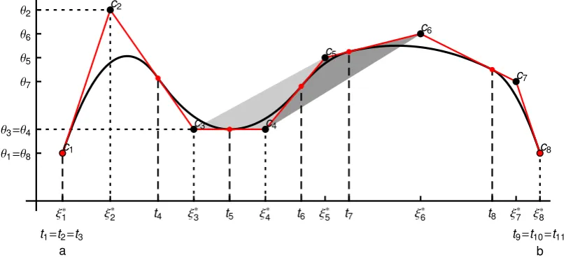
Q∗(t), denoted byCQ∗(t), (see Figure 1). This relationship is due to the fact that both the x

andycoordinates of the control points ci,i= 1, . . . , p, are related to the spline regression curve

Q∗(t). More precisely, thex-coordinates,ξ∗_i, are the Greville sites (4), obtained from the knots

tk,n, and they-coordinates,θi, are simply the spline regression coefficients. Due to the partition

of unity property of B-splines, ∑j_i=j−n+1Ni,n(t) = 1 for any t ∈ [tj, tj+1), j = n, . . . , n+k,

the curve Q∗(t) of ordernis a convex combination ofn of its control points, and its graph lies

within the convex hull of its control polygon CQ∗. The convex hull ofc1, . . . ,cp is the smallest

convex polygon, enclosing these points. Thus, the higher is the degree,n−1, the stronger is the

curve’s deviation from its control polygon CQ∗, but it still remains within the convex hull of

CQ∗. This suggests that a quadratic B-spline curve is very well suited as a compromise between

smoothness and shape preservation. Hence, due to the convex hull property, the curve is in

a close vicinity of its control polygon as illustrated in Figure 1 with respect to two adjacent

polynomial segments ofQ∗(t). The grey areas in Figure 1 are the two convex hulls, formed by

c3,c4,c5 and c4,c5,c6, within which the two segments of Q∗(t), for t∈[t5, t6] and t∈[t6, t7],

c₁

c2

c3 c4

c5

c₆

c₇

c₈

Ξ1* t₁₌t₂₌t₃

a Ξ2 * Ξ3 * Ξ4 * Ξ5 * Ξ6 * Ξ7 *

t4 t5 t6 t7 t8 Ξ8*

t₉₌t₁₀₌t₁₁ b

Θ1=Θ8

Θ2

Θ3=Θ4

Θ5

Θ6

[image:8.595.94.499.90.276.2]

Θ7

Figure 1: A quadratic (n = 3), functional spline regression curve Q∗(t), with k = 5 internal knots, and its control polygon CQ∗(t). The spline coefficients θ and the set of knots t5,3 are

arbitrarily chosen, and the Greville sites ξ∗(t5,3) are evaluated following (4).

and hence can be expressed as

CQ∗(t) =

{ _p

∑

i=1

ξ_i∗Ni,2(t),

p ∑

i=1

θiNi,2(t)

} = { t, p ∑ i=1

θiNi,2(t)

} ≡

p ∑

i=1

θiNi,2(t). (7)

In (7),∑p_i=1ξ_i∗Ni,2(t) =tsinceNi,2(t) are defined over the knotstp−2,2, wheret1 ≡ξ1∗,tp+2 ≡ξp∗

and ti+1 ≡ ξi∗, i = 1, . . . , p and the linear precision property (5) applies. For further details

related to geometric modelling with splines we refer to Cohen et al. (2001).

Next, we emphasize that the spline regression curve Q∗(t) not only lies within the convex

hull of CQ∗(t) but it follows its shape. That is, because Q∗(t) is the Schoenberg’s variation

diminishing spline approximation of its control polygonCQ∗(t), i.e.

V [CQ∗] (t) =

p ∑

i=1

CQ∗(ξ∗i)Ni,n(t) = p ∑

i=1

θiNi,n(t)≡Q∗(t), (8)

whereξ_i∗,i= 1,2, . . . , p, are the Greville abscissae, obtained fromtk,n andCQ∗(ξi∗) =θi by the

definition of the control polygon. Given a set of knots, tk,n, the spline approximation

V[g](x) =

p ∑

i=1

g(ξ_i∗)Ni,n(x) (9)

(VDS) approximation of order n to g, on the set of knots tk,n, see e.g. De Boor (2001). It is

constructed by simply evaluating g at the Greville sites (4) and taking the values g(ξ_i∗) as the

B-spline coefficients of the VDS approximation.

It is important to recall a property ofV[g], which is crucial for developing the GeD estimator.

That is, the VDS approximation, V[g] is shape preserving since it preserves the shape of the

function g it approximates. More precisely, if g is positive, then V[g] is also positive, if g is

monotone, then V[g] is also monotone, and if g is convex, V[g] is also convex. The variation

diminishing character ofV[g] is due to the fact that it crosses any straight line at most as many

times as does the functiongitself. In view of the convex hull property and the shape preserving

property of (8) it is now clear that Q∗(t) not only lies close to its control polygon CQ∗(t) but

also preserves its shape. In fact, in the linear case, i.e., when n = 2, the parametric curve,

Q∗(t) defined by (6) coincides with its control polygonCQ∗(t), i.e., Q∗(t) =CQ∗(t), since the

Greville sites in (4) coincide with the knots, i.e. ξ_i∗=ti+1,i= 1, . . . p.

In summary, it has been established that the spline regression function f(tk,n,θ;x),

(alter-natively denoted as Q∗(x), x ∈ [a, b]), can be expressed in the form (6) and that its control

polygon, Cf(tk,n,θ;x), has vertices ci = (ξi∗, θi), i = 1, . . . , p, where ξ∗i are the Greville sites

(4), obtained from tk,n. The latter suggests that, given n and k, locating the knots tk,n and

finding the regression coefficients θ off(tk,n,θ;x), based on the set of observations {yi, xi}Ni=1,

is equivalent to finding the location of the x- and y-coordinates of the vertices of Cf(tk,n,θ;x).

This establishes the important fact that estimation of tk,n and θ affects the geometrical

po-sition of the control polygon C_f(tk,n,θ;x), which, due to the shape preserving and convex hull

properties, defines the location of the spline curve f(tk,n,θ;x). Inversely, locating the vertices

ci of Cf(tk,n,θ;x) affects the knots tk,n, through (4), and the values of θ, and hence affects the

position of the regression curvef(tk,n,θ;x). The latter conclusion motivates the construction,

in stage A of GeDS, of a control polygon as a linear least squares spline fit to the data, whose

knots determine the knotstk,n, and whose B-spline coefficients are viewed as an initial estimate

of θ, which is improved further in stage B (see section 3). This is the basis of our approach

to constructing the GeD variable knot spline approximation to the unknown functionf in (1),

3

Geometrically designed spline regression.

In this section, we introduce the GeD spline regression method which is motivated by the ideas,

outlined in section 2. The method “positions” first an initial control polygon (linear spline fit),

which reproduces the “shape” of the data, applying least squares approximation. Secondly,

an optimal set of knots of a higher order (n > 2) smooth spline curve is found, so that it

preserves the shape of the initial control polygon and then this curve is fitted to the data,

to adjust its position in the LS sense. In this way, it is ensured that the n-th order smooth

LS fit follows the shape of the initial control polygon, and hence the shape of the data. This

procedure simultaneously produces linear, quadratic, cubic, or higher order splines and the LS

fit with the minimum residual sum of squares is chosen as the final fit which recovers best

the underlying unknown functionf. It should be mentioned that all the fits (linear, quadratic

etc.) are constructed so that they have dimension p equal to the dimension of the linear fit

constructed first. This is achieved by positioning the knots of the higher order, (n >2) spline

fits according to the averaging relation (20), as described in section 3.1. The two stages of the

GeDS approach may be given a formal interpretation as certain optimization problems with

respect to the variablesk,tk,n,θ andn.

Stage A. Starting from a straight line fit and adding one knot at a time, find the least

squares linear spline fit ˆf(δl,2,αˆ;x) =

∑p

i=1αˆiNi,2(x) with a number of internal knotsl, number

of B-splines p=l+ 2 and with a set of knots δl,2 ={δ1=δ2 < δ3< . . . < δl+2 < δl+3 =δl+4},

such that the ratio of the residual sums of squares

RSS(l+q)/RSS(l) =

N ∑

j=1

(

yj −fˆ(δl+q,2;xj)

)2/∑N

j=1

(

yj−fˆ(δl,2;xj) )2

≥α_exit (10)

where q≥1 and α_{exit is a certain threshold level. Testing the inequality in (10) serves as the}

stage A model selector. If the inequality in (10) is fulfilled, ˆf(δl,2,αˆ;x) could not be significantly

improved if q more knots are added and ˆf(δl,2,αˆ;x) is the selected model which adequately

reproduces the “shape” of the unknown, underlying function f.

In order to realize stage A, a locally-adaptive knot insertion scheme is proposed. It starts

from an LS fit, in the form of a straight line segment, as described in step 1 below. The latter

those points, where the fit deviates most from the shape of the underlying function, (see Figure

2), according to a bias driven measure of appropriately defined clusters of residuals (see steps 2

- 8). A stopping rule is introduced, which serves as a model selector and allows us to determine

the appropriate number and location of the knots of the linear spline fit ˆf(δl,2,αˆ;x) (see steps

9 - 10). A formal description is given next.

Step 1. Let n = 2, k = 0. Find the LS spline fit ˆf(δ0,2,αˆ;x) = ˆα1N1,2(x) + ˆα2N2,2(x),

where δ0,2 = {δi}4_i=1 with a = δ1 = δ2 < δ3 = δ4 = b. Calculate the residuals ri ≡ r(xi) =

yi−fˆ(δ0,2,αˆ;xi), i = 1, . . . , N and the residual sum of squares RSS(k) =

∑N

i=1r2i of the fit

withk internal knots.

Step 2. Group the consecutive residualsri,i= 1, . . . , N into clusters by their sign, i.e. find

a number u, 1 ≤u ≤ N and a set of integer values dj >0, j = 1, . . . , u such that sign(r1) =

. . .=sign(rd1) ̸=sign(rd1+1) =sign(rd1+2) =. . .=sign (rd1+d2)̸=. . .̸=sign(rd1+d2+···+du−1+1) =

sign(rd1+d2+···+du−1+2) =. . .=sign(rd1+d2+···+du), and ∑u

j=1dj =N.

Step 3. For each of theuclusters of residuals of identical signs, calculate the within-cluster

mean residual value

mj =  

dj ∑

i=1

rd(j−1)+i 

/dj = dj ∑

i=1

( (

ˆ

fd(j−1)+i−Efˆd(j−1)+i )

+

(

Efˆd(j−1)+i−fd(j−1)+i )

+ϵd(j−1)+i )/ dj = dj ∑ i=1 ( ˆ

fd(j−1)+i−Efˆd(j−1)+i )

/dj+ dj ∑

i=1

(

Efˆd(j−1)+i−fd(j−1)+i )

/dj+ dj ∑

i=1

ϵd(j−1)+i/dj,

j= 1, . . . , u, whered(j) =d1+d2+· · ·+dj and the three terms in the last decomposition can

be interpreted as the within-cluster average variance, bias, and error, respectively. Calculate

also the within-cluster range (withd(0) = 0)

ηj =xd(j)−xd(j−1)+1, j= 1, . . . , u.

Step 4. Findmmax = max1≤j≤u(mj) andηmax = max1≤j≤u(ηj) and calculate,

correspond-ingly, the normalized within-cluster mean and range valuesm′_j =mj/mmax andη′j =ηj/ηmax,

Step 5. Calculate the cluster weights

wj =βm′j+ (1−β)η′j, j = 1, . . . , u, (11)

where, β is a real valued parameter, 0 ≤ β ≤ 1. The value wj serves as a measure, attached

to the j-th cluster of residuals of identical sign, which measures the deviation of the current

least squares linear spline fit ˆf(δk,2,αˆ;x) fromf in thej-th cluster. The weight β is one of the

parameters whose value needs to be chosen at the start of stage A.

Step 6. Order the weights of the clusters, i.e. wj1 ≥wj2 ≥. . . ≥ wju. Thus, in order to

improve ˆf(δk,2,αˆ;x), in the next step a new knot is inserted, at an appropriate location, within

thej1-th cluster.

Step 7. Check whether there is already a knot within thej1-th cluster, i.e. check whether

δi ∈ [

xd(j1−1)+1, xd(j1−1)+dj₁ ]

, for each internal knot δi ∈ δk,2, i = 3, . . . , k+ 2. If there is

already a knot within the j1-th cluster, the check is repeated for the cluster with index j2, and

so on until the first cluster, say indexedjs, is found which does not contain a knot. Then, insert

a new knotδ∗ at the site

δ∗=

 

d(js−∑1)+djs

i=d(js−1)+1

rixi  / 

d(js−∑1)+djs

i=d(js−1)+1

ri 

. (12)

Note that δ∗ ∈

[

x_d(js−1)+1, x_{d(js−1)+djs}

]

. The new knot position (12) can be viewed as a

weighted average of thex-coordinates of the residuals in thejs-th cluster, the weights being the

normalized values of the residuals. The set of knotsδk,2is being updated asδ∗k+1,2 :=δk,2

∪ {δ∗}.

So, a new knot is placed where the cluster weight (11) is maximal. In view of the

decom-position in step 3, the cluster weight (11) can be referred to as a bias dominated measure since

the bias component is dominant in this cluster compared to the variance and error terms (at

least at the initial iterations when there are small number of knots in the linear fit and the

approximation error is large).

Step 8. Find the least squares linear spline fit

ˆ

f(δ∗_k+1,2,αˆ;x)=

p ∑

i=1

ˆ

Since δ∗_k+1,2 contains the new knot, the number of B-splines,p, will increase by one.

Step 9. Calculate the residuals ri, i = 1, . . . , N and the RSS(k+ 1) for ˆf (

δ∗_k+1,2,αˆ;x).

Note thatδk,2⊂δ∗k+1,2 implies thatSδk,2 ⊂Sδ∗k+1,2. Hence ˆf(δk,2,αˆ;x)∈Sδ∗k+1,2 and applying

the orthogonality property of least squares estimation it is easy to see that

N ∑

i=1

(

yi−fˆ(δk,2,αˆ;xi) )2

=

N ∑

i=1

(

yi−fˆ (

δ∗_k+1,2,αˆ;xi ))2

+

N ∑

i=1

(

ˆ

f(δ∗_k+1,2,αˆ;xi )

−_fˆ_{(δk,2,αˆ;xi)})2_.

(13)

Equation (13) implies that RSS(k+ 1)<RSS(k). It is obvious also that RSS(k) will converge to

zero ask+n→N since whenk+n=N the fit interpolates the data. The greedy fashion of

the new knot placement (12), combined with equation (13), gives rise to the rule for exit from

stage A of the GeDS method, given next.

Step 10. Letq ≥1 be a fixed integer, chosen at the beginning of stage A. Ifk≤q go back

to step 2, otherwise calculate the ratio

α= RSS(k+ 1)/RSS(k+ 1−q).

Note that from (13) it follows that 0< α <1. Ifα ≥α_{exit, an exit from stage A is performed}

with the spline fit ˆf(δl,2,αˆ;x),l=k+ 1−q. Ifα < α_{exit then}fˆ

(

δ∗_k+1,2,αˆ;x) is taken as the

current fit and the procedure goes back to step 2. The valueα_{exit is chosen ex ante to be close}

to 1. This is because the ratio α will be close to zero if the fit has improved significantly by

adding δ∗ and will tend to 1 if no improvement has been achieved in the last q+ 1 consecutive

iterations, i.e the corresponding values of the RSS have stabilized. Our experience has shown

that this stopping rule works well as a model selector with q = 2, i.e., stabilization of RSS in

three consecutive iterations is sufficient to exit from stage A with the appropriate number of

knots.

Remark 3.1 Let us note that in the Normal error case, i.e. when ϵ ∈ N (0, σ2

ϵ )

, the

log-likelihood, logL(δk,2), of a current linear spline fit fˆ(δk,2,αˆ;x) with k knots is proportional to

its corresponding residual sum of squares, RSS(k), i.e. logL(δk,2)∝-RSS(k) (see e.g. relation

(6) of Hansen and Kooperberg 2002). Therefore, the ratio of RSS in the left-hand side of (10)

can be interpreted as the ratio of the log-likelihoods of the two nested spline fits fˆ(δl+q,2,αˆ;x)

Remark 3.2 The knot insertion scheme in stage A can be described as a “greedy” one (see

Hastie 1989), since at each iteration it places a knot, δ∗, where a within-cluster bias dominated

measure is maximal (see steps 3 and 5), which is very near to the site where placing a knot

gives the largest reduction in the residual sum of squares. This can be quantified using the fact

that given an LS fit fˆ(δk,2;x), with 0 < k < l internal knots, if a knot, δ∗, is added in the

interval [δj∗, δj∗+1],2≤j∗ < k+ 2, then the updated LS fit fˆ

(

δ∗_k+1,2;x) adjusts best to the data

in[δj∗, δj∗+1], sincefˆ(δk,2;x)−fˆ

(

δ∗_k+1,2;x),x∈[δj, δj+1]decreases exponentially in |j∗−j|,

which is the number of knots between x andδ∗. This follows from Theorem 1 of Zhou and Shen

(2001).

As an alternative to the model selector in (10), (see also step 10 of stage A), we have implemented

two additional model selection criteria based on the minimization of SURE and GCV. More

precisely, the GeD linear spline fit with number of knots k = k_{min which minimizes Stein’s}

unbiased risk estimate (SURE)

R( ˆf) =

N ∑

i=1

(

yi−fˆ(δk,2,αˆ;xi) )2/

N+Dk+n N σ

2 ₍₁₄₎

or the generalized cross validation

GCV( ˆf) =

( _N

∑

i=1

(

yi−fˆ(δk,2,αˆ;xi) )2/

N

) / (

1−d(k)

N

)2

(15)

criterion is selected as the outcome of stage A. We have assumed that the minimum is attained

when SURE or GCV do not decrease in two consecutive iterations in stage A. Criteria (14) and

(15) depend on the choice of the parametersD and d(k), and whenD= 1.2 and d(k) =k+ 1

they behave roughly as the criterion in (10), as illustrated by Figure 5 (a) and the related results

in the online supplement. The choice D = 3 and d(k) = 3k+ 1, as noted by Zhou and Shen

(2001) tends to yield a model underfitting the underlying function f. In section 4 and in the

online supplement to the paper, we give a comparison of the three model selection approaches,

(10), (14) and (15), and a thorough sensitivity study of the GeD spline estimation with respect

to the choice of the free parameters,α_{exit and} β (see steps 10 and 5 of stage A).

If a smoother fit is needed, the linear LS spline fit ˆf(δl,2,αˆ;x) is viewed as a control polygon

constructed in stage B, based on the geometrical form of ˆf(δl,2,αˆ;x).

Stage B.1. For each of the values of n = 3, . . . , nmax, find the optimal set of knots

˜_{tl−(n−2),n, as a solution of the constrained minimization problem}

min

tl−(n−2),n, δi+2<ti+n<δi+n, i=1,...,(l−(n−2))

_fˆ_{(δl,2,αˆ;x)−C}

f(tl−(n−2),n,αˆ;x)

∞, (16)

where∥g∥_∞:= maxa≤x≤b|g(x)|is the uniform (L∞) norm of a functiong(x). In fact,

minimiza-tion in (16) gives the polygonC_f(˜tl−(n−2),n,αˆ;x) with vertices (ξ ∗

i,αˆi), so that

ξ_i∗(˜tl−(n−2),n)≃δi+1, i= 1, . . . , p (17)

or equivalently, so that

t=

p ∑

i=1

ξ_i∗Ni,n(t)≃ p ∑

i=1

δi+1Ni,n(t). (18)

Remark 3.3 Achieving exact equality in (17), respectively (18), is impossible in general since

expressing ξ_i∗(tl−(n−2),n) following (4), we have that,ξ1∗ =δ2 =a, ξ∗p =δp+1 =b and

δi+1 = (ti+1+. . .+ti+n−1)/(n−1), i= 2, . . . , p−1, (19)

which is an over-determined system ofp−2 =lequations andl−(n−2)ordered, unknown knots,

tl−(n−2),n,(n >2). Instead, what is achieved by solving (16) is thatCf₍˜tl−(n−2),n,αˆ;x) is as close

to fˆ(δl,2,αˆ;x) as possible becauseξ∗(˜tl−(n−2),n) is as close to δl,2 as possible. Note that, since

we viewδi+1, i= 1, . . . , p, as Greville sites of a higher order spline functionf

(

tl−(n−2),n,αˆ;x )

,

the constraints δi+2< ti+n< δi+n, i= 1, . . . ,(l−(n−2))in (16), follow from (19).

In summary, the objective of stage B is to produce a set of optimal knots˜tl−(n−2),n, which ensures

that ˆf(δl,2,αˆ;x) becomes (nearly) the control polygon of the spline functionf

(

˜_{tl−(n−2),n,αˆ;x})_,

i.e. thatC_f(˜tl−(n−2),n,αˆ;x) ≃

ˆ

f(δl,2,αˆ;x). Or equivalently,˜tl−(n−2),nis placed so thatf (_˜

tl−(n−2),n,αˆ;x )

becomes (nearly) the Schoenberg’s VDS approximation of ˆf(δl,2,αˆ;x). Therefore, due to its

convex hull and shape preserving properties (see section 2), f(˜t_{l−(n−2),n},αˆ;x) lies very close

to ˆf(δl,2,αˆ;x), and hence to the “shape” of the data for which the linear LS approximation

place-ment in Stage B of GeDS. The fact that f(˜tl−(n−2),n,αˆ;x )

is nearly a VDS approximation of

ˆ

f(δl,2,αˆ;x) has been quantified with appropriate error bounds but due to volume limitation

these are omitted, and bounds are only given for the knot location t_{l−(n−2),n} as described in

the next section 3.1.

However, we note that f(˜t_{l−(n−2),n},αˆ;x) is not a least squares approximation to the data

set. In order to obtain a least squares fit to the data and at the same time to preserve the

shape of f(˜tl−(n−2),n,αˆ;x )

, its optimal knots ˜tl−(n−2),n are preserved, whereas its B-spline

coefficients,αˆ, are released and are assumed to be unknown parameters,θ, which are estimated

in the least squares sense, using {xi, yi}Ni=1, as follows.

Stage B.2. For a fixedn= 3, . . . , nmax, find the least squares fit ˆf

(

˜_{tl−(n−2),n,θ}ˆ_;x)_which

solves

min θ

N ∑

j=1

(

yj−f (_˜

t_{l−(n−2),n},θ;xj ))2

.

Among all fits ˆf

(

˜_{tl−(n−2),n,θ}ˆ_;x)_{, of order n = 2, . . . , nmax, i.e. including the linear fit,}

ˆ

f(δl,2,αˆ;x) from stage A, choose the one of order ˆn, for which the RSS is minimal.

In this way in stage B.2, along with the number of knots and their locations, the degree of

the spline is also estimated. This is an important feature of the proposed estimation method

which is rarely offered by other spline estimation procedures. One alternative that we are aware

of is the MDL method of Lee (2000) (see also Lee 2002a,b). Of course, any of the produced final

fits of order n ̸= ˆn could be used, if other features were more desirable, for example if better

smoothness were required.

3.1 Stage B.1 - Approximate solution: the averaging knot location.

The minimization problem (16), of stage B.1, is a constrained non-linear optimization problem

with respect to the knots and although it is related to linear splines, it is still computationally

involved. In addition, as with any other non-linear optimization problem, finding the globally

optimal solution is not guaranteed. The knots˜tl−(n−2),n, which are the optimal solution, may

also be (almost) coalescent and this may cause edges and corners in the final LS fit in stage B.2.

In order to avoid these undesirable features, but to preserve the optimality properties of the

knots, as described in stage B.1, we propose to place the knots in stage B.1 according to (20),

solution to the minimization problem (16), respectively (19). Thus, the final GeD spline fit

from stage B.2 is ˆf

(

¯_{tl−(ˆn−2),ˆn,θ}ˆ_;x)_{, where}¯_{tl−(ˆn−2),nˆ is given by (20) with n= ˆn.}

The averaging knot location: Given the control polygon ˆf(δl,2,αˆ;x) of stage A, for

each n = 3, . . . , n_{max, calculate the knot placement}¯t_{l−(n−2),n} with internal knots defined as

the averages of the knots, δl,2, i.e.,

¯

ti+n= (δi+2+· · ·+δi+n)/(n−1), i= 1, . . . , l−(n−2). (20)

The choice of the knots¯t_{l−(n−2),n} according to (20) makes it possible to establish appropriate

error bounds given by Corollaries 3.5 and 3.6 of Theorem 3.4, the proofs of which are provided

in Appendix A.

Theorem 3.4 Let {ξi}p_i=1 be an ordered set, a = ξ1 < ξ2 < . . . < ξp = b, and let tk,n,

(p≥n≥2,k=p−n), be a set of knots, defined as in (2), with

ti+n= (ξi+1+· · ·+ξi+n−1)/(n−1), i= 1, . . . , k. (21)

Then, for the n-th order spline approximation Va[g], defined on tk,n, of a continuous function

g∈C[a, b], given by

Va[g](x) =

p ∑

i=1

g(ξi)Ni,n(x), (22)

we have

∥V[g]−Va[g]∥_∞≤

⌈

(n−2)2 2(n−1)

⌉

ω(g;max_{j∈{1,...,p−1}}(ξj+1−ξj)), (23)

where ⌈ν⌉:=min{z∈Z:ν ≤z},V[g]is the Schoenberg’s VDS approximation, defined on tk,n

and

ω(g;h) :=max{|g(x)−g(y)|:|x−y| ≤h, x, y∈[a, b]} (24)

is the modulus of continuity of the function g ath.

Corollary 3.5 Under the assumptions of Theorem 3.4, with n = 3, ξi replaced by δi+1, i =

1, . . . , p, p=l+ 2, k=l−(n−2) and ifg coincides with the straight linet, i.e. g≡t, then

∥V[t]−Va[t]∥_∞=

t−

p ∑

i=1

δi+1Ni,n(t)

∞

≤ (n−2)2

Corollary 3.6 Under the assumptions of Theorem 3.4, with ξi replaced by δi+1, i = 1, . . . , p,

p=l+ 2, k=l−1,ξ∗(tl−1,3), and assuming that g is the linear spline functionfˆ(δl,2,αˆ;x) =

∑p

i=1αˆiNi,2(t) with vertices (δi+1,αˆi), we have

∥V[ ˆf]−Va[ ˆf]∥_∞ =

p ∑

i=1

ˆ

f(δl,2,αˆ;ξi∗)Ni,3(x)−

p ∑

i=1

ˆ

f(δl,2,αˆ;δi+1)Ni,3(x)

∞

≤ 1

4maxj∈{2,...,p−1}|αˆj −αˆj−1|. (26)

We have performed a special simulation study, which illustrates that bound (25) is quite tight

(best for n = 3) and that the averaging knot location (20) gives a reasonably accurate

ap-proximation to the solution of system (19). Due to volume limitations, details of this study are

relegated to the online supplement of the paper (see section 1.2 therein). Furthermore, following

Huang (2003) one can also study the local asymptotic properties of the proposed GeD spline

estimator, but this is beyond the scope of this paper.

4

Numerical Study.

In this section, and in the online supplement to the paper, we illustrate the numerical

per-formance of the GeDS method and its properties, established in section 3, both on simulated

and real data examples. We have performed a thorough simulation study of the impact on

the GeDS knot location and related MSE (mean square error), of different assumptions and

choices made in constructing the GeDS estimate, namely, different levels of the signal to noise

ratio (SNR from 2 to 7), sample sizes (N = 90,150,256,512,2048) and levels of smoothness

of the underlying function (smooth, medium smooth and wiggly functions), different choices of

the GeDS parameters, α_{exit and} β, (α_{exit = 0}.8,0.9,0.95,0.99,0.995,0.999, β = 0.3,0.5,0.7)

different choice of the model selection criterion (GeDS criterion, GCV and SURE), and different

degree of the GeD spline estimate (linear, quadratic and cubic). We have also tested the GeDS

knot selection strategy versus equally spaced knots and other established approaches (see the

real data example of section 4 and the test examples in the online supplement). We have tested

GeDS on a series of simulated examples, used in many other studies on variable knot spline

methods (cf. Schwetlick and Sch¨utze 1995, Fan and Gijbels 1995, Donoho and Johnstone 1994

simulated test functions, given in Table 1, first considered by Schwetlick and Sch¨utze (1995),

and one real data example from materials science, due to Kimber et al. (2009). The detailed

results related to the other test functions are given in the online supplement to this paper, see

Tables 1 and 2 therein.

As specified in section 3, there are two parameters, α_exit∈(0,1) and β ∈(0,1), defined in

steps 10 and 5 of stage A of GeDS, by means of which the model selection can be controlled. The

parameterα_{exit is related to the model selection rule which determines when to exit from stage}

A, i.e. it determines the number of knots, l, in the set δl,2 of the linear spline fit ˆf(δl,2,αˆ;x)

and hence, the number of knots of the final higher order LS spline fit ˆf

(

¯_{tl−(n−2),n,θ}ˆ_;x)_{. The}

parameter β determines the weight put on the cluster range and the mean cluster size within

each cluster of residuals of same sign, as specified in step 5 of stage A. It therefore affects to

some extent the ordering of the cluster weights and hence, the knot placement.

As can be presumed, the choice ofβ depends on the level of the signal-to-noise ratio (SNR),

SNR= (var(f))0.5/σϵ and on the degree of smoothness/wiggliness of f. As can be concluded

from the performed numerical tests, when the SNR is high and f is smooth, recommended

values are β ∈[0.5,0.7], α_exit ∈[0.9,0.95]. If the SNR is high and f is a wiggly function then

the recommended choice isβ ∈[0.5,0.7],α_exit∈[0.99,0.995], since otherwise underfitting may

result. In the case when SNR is low and f is smooth, one may use β ∈ [0.3,0.5], α_exit ∈

[0.9,0.95]. Finally, it is known that when the SNR is low and the underlying function is very

unsmoothy recovering f is very difficult and different choices of β and α_{exit may need to be}

attempted.

In summary, in most numerical examples (see section 4.1 and the online supplement), GeDS

produces very good results avoiding over and under fitting with values α_exit ≥ 0.9, β = 0.5.

Recall, β = 0.5 means that the within-cluster mean residual value and the cluster range are

considered equally important components of a cluster weight. Our experience shows that choices

of α_exit ∈(0,0.8) generally lead to underfitting, especially for less smooth functions. Thus, in

order to obtain a GeDS estimate it is necessary to input only the set of data{xi, yi}Ni=1 and use

4.1 A simulated example.

In this section, we aim at illustrating the method and its properties on the following test

example, which appears in Schwetlick and Sch¨utze (1995). The proposed GeDS method has

been implemented using Mathematica 9.0 and a standard PC (Intel core i7 CPU, 2.93 Ghz,

[image:20.595.68.540.220.285.2]

8GB RAM) has been used for all test examples. For a simulated data set, graphs of the linear

Table 1: Test function.

Test function Interval Sample size, N xi,i= 1, . . . , N Noise level,σϵ SNR

f(x) = ₁₊₁₀₀10x_x2 [-2,2] 90 xi=−2 +2−₈₉(−2)(i−1) U(−0.05,0.05) 7

180 U(−0.05,0.05) 7

180 U(−0.065,0.065) 5

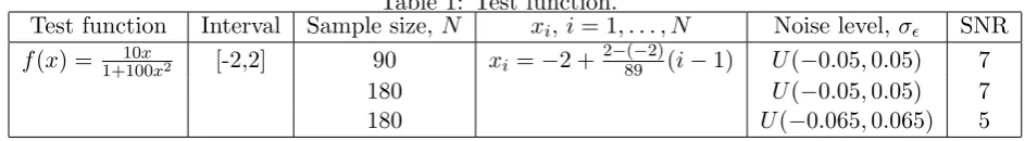
spline fits, produced at each consecutive iteration in stage A of GeDS, preceding the final one,

are given in Figure 2. As can be seen, the initial straight line fit, presented in Figure 2 (a), is

sequentially improved by adding knots, one at each iteration, to reach the fit ˆf(δ8,2;x), plotted

in Figure 3 (a), which can not be further significantly improved by adding more knots. Applying

the averaging knot location (20) to the knotsδ8,2, the set of knots¯t8−(n−2),n of the quadratic,

n= 3, and cubic, n= 4, fits, ˆf(¯t8−(n−2),n;x )

, are defined as follows: ¯t4 = (−1.1−0.33)/2 =

−0.69, ¯t5 = (−0.33−0.12)/2 = −0.22, . . . in ¯t7,3, or ¯t5 = (−1.1−0.33−0.12)/3 = −0.51,

¯

t6 = (−0.33−0.12−0.05)/3 =−0.17,. . .in¯t6,4. The LS spline fits ˆf

(

¯_{t8−(n−2),n,θ}ˆ_;x)_{, resulting}

from stage B of GeDS, are plotted in Figure 3 (b) and (c) for n= 3 and n= 4, respectively.

The polygonsC_f(˜t

7,3,αˆ;x) andCf(¯t7,3,αˆ;x), plotted in Figure 3 (d), using dot-dashed and dashed lines, and obtained with˜t7,3 as the solution of (16) and with¯t7,3, calculated using (20), are seen

to be very close to each other and also close to the initial control polygon ˆf(δ8,2,αˆ;x). The

LS fits, ˆf(˜t7,3;x

)

and ˆf(¯t7,3;x), have close L2-errors, respectively 0.2798 and 0.2944, which

confirms that¯t7,3 approximates very well the optimal set of knots˜t7,3. TheL2-error is defined

as the square root of the sum of squared residuals. The details of the final linear fit, and its

corresponding quadratic and cubic spline fits are presented in Table 2. As can be seen, the

function f is symmetric and GeDS places, symmetrically around the origin, 8, 7 and 6 knots,

respectively for the linear, quadratic and cubic LS fits. All the fits are of a very good quality

with respect to the mean square error (MSE), defined as MSE=

{_∑

N i=1

(

f(xi)−fˆ(xi) )2}

/N.

Based on the L2-errors for fits 1-3 given in Table 2, the best GeDS fit for this particular data

-2 -1 0 1 2 -0.6 -0.4 -0.2 0.0 0.2 0.4 0.6

HaL ∆_0,2=8<

-2 -1 0 1 2

-0.6 -0.4 -0.2 0.0 0.2 0.4 0.6

HbL ∆_1,2=80.32<

-2 -1 0 1 2

-0.6 -0.4 -0.2 0.0 0.2 0.4 0.6

HcL ∆_2,2=8-0.33, 0.32<

-2 -1 0 1 2

-0.6 -0.4 -0.2 0.0 0.2 0.4 0.6

HdL ∆_3,2=8-0.33, 0.12, 0.32<

-2 -1 0 1 2

-0.6 -0.4 -0.2 0.0 0.2 0.4 0.6

HeL

∆_4,2=8-0.33,-0.12, 0.12, 0.32<

-2 -1 0 1 2

-0.6 -0.4 -0.2 0.0 0.2 0.4 0.6

HfL

∆_5,2=8-1.1,-0.33,-0.12, 0.12, 0.32<

-2 -1 0 1 2

-0.6 -0.4 -0.2 0.0 0.2 0.4 0.6

HgL

∆_6,2=81.1,-0.33,-0.12, 0.05, 0.12, 0.32<

-2 -1 0 1 2

-0.6 -0.4 -0.2 0.0 0.2 0.4 0.6

HhL

[image:21.595.85.511.76.716.2]

∆_7,2=8-1.1,-0.33,-0.12, 0.05, 0.12, 0.32, 0.96<

-2 -1 0 1 2

-0.4

-0.2 0.0 0.2 0.4

HaL

∆_8,2=8-1.1,-0.33,-0.12,-0.05, 0.05, 0.12, 0.32, 0.96<

-2 -1 0 1 2

-0.4

-0.2 0.0 0.2 0.4

HbL

-2 -1 0 1 2

-0.4

-0.2 0.0 0.2 0.4

HcL

-2 -1 0 1 2

-0.4

-0.2 0.0 0.2 0.4

[image:22.595.84.516.135.451.2]

HdL

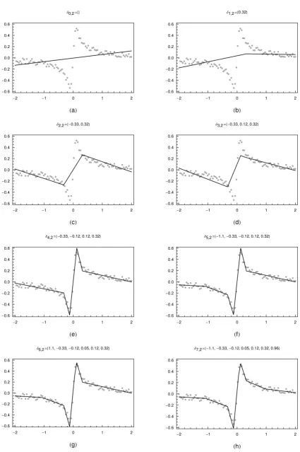
Figure 3: The final GeD spline fits: (a) linear, ˆf(δ8,2,αˆ;x); (b) quadratic, ˆf

(

¯_t7,3,θˆ_;x)_{; (c)}

cubic, ˆf

(

¯_t6,4,θˆ_;x)_{; (d) graphs of ˆf(δ8,2,αˆ;x) - the solid line,C}

[image:22.595.71.540.622.713.2]

f(˜t7,3,αˆ;x) - the dot-dashed line and C_f(¯t7,3,αˆ;x) - the dashed line; The dotted curve in (a), (b), (c) is the true function.

Table 2: Summary of GeD (No 1-3) and PNOM and NOM spline fits. N = 90, SNR= 7.

No Fit n k Internal knots α_exit, β L2-error, MSE

1 Fig. 4,(a) 2 8 {-1.1,-0.33,-0.12,-0.05,0.05,0.12,0.32,0.96} 0.9,0.5 0.2699,0.000189 2 Fig. 4,(b) 3 7 {-0.69,-0.22,-0.09,0.00,0.09,0.22,0.64} 0.9,0.5 0.2944,0.000127 3 Fig. 4,(c) 4 6 {-0.51,-0.17,-0.04,0.04,0.16,0.47} 0.9,0.5 0.2631,0.000119

4 PNOM 4 6 {-0.53,-0.16,-0.06,0.05,0.17,0.51} - 0.2623,0.000131

obtained applying the LS non-linear optimization method (NOM) and its penalized version

(PNOM), due to Lindstrom (1999). As can be seen, the three fits are very close, comparing

the L2-errors, the MSE and the location of the knots. However, the GeD fit recovers best the

original function as indicated by the corresponding MSE values. The computation time for the

three GeDS fits is 0.87 seconds whereas for PNOM and NOM it is respectively, 4.5 hours and

1.4 hours, using the Mathematica functionNMinimize.

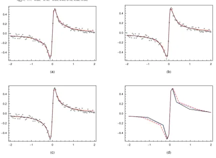
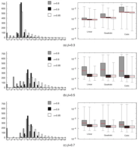
On this example, we test GeDS by fitting 1000 simulated data sets. Frequency plots of the

number of internal knots of the 1000 linear GeD spline fits and box plots of the MSE values

of the linear, quadratic and cubic GeDS fits are presented in Figure 4, for choices of values of

the parameter α_{exit = 0}.8,0.9,0.95, and choices for parameterβ = 0.3,0.5,0.7. The frequency

plots given on the left panels of Figure 4 show that for this test example a choice ofα_{exit = 0}.8

leads to a relative underfitting, whereas setting α_{exit = 0}.95 results in overfitting, regardless

of the level of the parameter β. The choice α_{exit = 0}.9 provides the best distribution of the

number of knots chosen for the linear fit at the end of Stage A, in particular whenβ = 0.5 or

β = 0.7. Recall that a higher value ofβ assigns more weight to the within-cluster mean relative

to the within-cluster range for clusters of residuals of same sign. The box plots presented in the

right panels of Figure 4 illustrate that, for the particular level of smoothness of the test function

and the chosen SNR=7, the results forβ = 0.5 andβ = 0.7 are substantially better than those

forβ = 0.3, with the cubic and the quadratic GeDS fits being very close for both α_{exit = 0}.9

and α_{exit = 0}.95. For levels of β = 0.7 andα_{exit = 0}.9 for instance, the 1000 linear, quadratic

and cubic GeD spline fits, with median number of regression functionsn+k= 10, have median

L2-errors 0.2604, 0.2679, 0.2637 (MSE values 0.000186, 0.000151, 0.000137) respectively, which

are slightly lower than 0.277, obtained by Schwetlick and Sch¨utze (1995) for a quartic (of order

5) fit with the same number of regression parameters and optimally located knots. The optimal

quartic fit of Schwetlick and Sch¨utze (1995) is obtained starting from 15 knots and after three

time-consuming knot generation, removal and relocation stages.

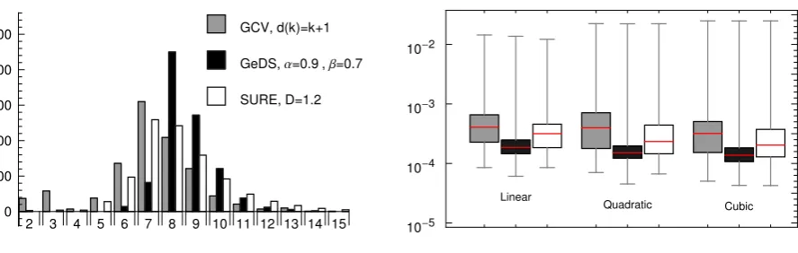
Continuing with the same test example, forN = 90 andSN R= 7, in Figure 5, the number

of knots and the MSE values for the 1000 GeD spline fits obtained withβ= 0.7 andα_{exit = 0}.9,

and illustrated in black on Figure 4 (c), are compared with the results obtained applying the

GeDS methodology to the same 1000 data sets but with two alternative model selection criteria,

2 3 4 5 6 7 8 9 10 11 12 13 14 15 16 17 18 19

Α=0.8

Α=0.9

Α=0.95

0 100 200 300 400 500 600 700

Linear

Quadratic

Cubic

10-2

10-3

10-4

10-5

HaLΒ=0.3

2 3 4 5 6 7 8 9 10 11 12 13 14 15 16 17 18 19

Α=0.8

Α=0.9

Α=0.95

0 100 200 300 400 500 600 700

Linear Quadratic

Cubic

10-2

10-3

10-4

10-5

HbLΒ=0.5

2 3 4 5 6 7 8 9 10 11 12 13 14 15 16 17 18 19

Α=0.8

Α=0.9

Α=0.95

0 100 200 300 400 500 600 700

Linear

Quadratic Cubic

10-2

10-3

10-4

10-5

[image:24.595.67.533.146.637.2]

HcLΒ=0.7

Figure 4: Frequency plots of the number of knots,l, (left panels) and box plots of the MSE values (right panels) of the 1000 GeD spline fits obtained with three different choices of values of the exit parameter α, and three choices of parameterβ illustrated on (a), (b) and (c) respectively.