Asymmetry through time dependency

DOI:10.1140/epjb/e2016-60639-0

Regular Article

PHYSICAL

JOURNAL

B

Asymmetry through time dependency

Alexander V. Mantzaris and Desmond J. Highama

Department of Mathematics and Statistics, University of Strathclyde, Glasgow G1 1XH, UK Received 5 August 2015 / Received in final form 8 November 2015

Published online 16 March 2016 c

The Author(s) 2016. This article is published with open access atSpringerlink.com

Abstract. Given a single network of interactions, asymmetry arises when the links aredirected. For example, if protein A upregulates protein B and protein B upregulates protein C, then (in the absence of any further relationships between them) A may affect C but not vice versa. This type of imbalance is reflected in the associated adjacency matrix, which will lack symmetry. A different type of imbalance can arise when interactions appear and disappear over time. If A meets B today and B meets C tomorrow, then (in the absence of any further relationships between them) A may pass a message or disease to C, but not vice versa. Hence, even when each interaction is a two-way exchange, the effect of time ordering can introduce asymmetry. This observation is very closely related to the fact that matrix multiplication is not commutative. In this work, we describe a method that has been designed to reveal asymmetry in static networks and show how it may be combined with a measure that summarizes the potential information flow between nodes in the temporal case. This results in a new method that quantifies the asymmetry arising through time ordering. We show by example that the new tool can be used to visualize and quantify the amount of asymmetry caused by the arrow of time.

1 Introduction

The success of Network Science as a research discipline shows that there is great value in studying a complex sys-tem through the connectivity of its components [1]. How-ever, even after simplifying down to the level of nodes and edges, there is typically too much information for us to digest, and we must rely on tools that further reduce the dimension of the system so that we can summarize and visualize key properties. The need to reveal hidden structure and substructure within a complex network has motivated a plethora of quantitative tools aimed at, for example, discovering significant nodes or edges, and topo-logical features such as well-connected communities, bi-partite structures, bottlenecks, motifs, hubs and authori-ties [2–9]. In this work we focus on the idea of quantifying and visualizing the level of asymmetry in a network, and in particular, studying asymmetry caused by the arrow of time in a dynamic network sequence.

First, we introduce some notation. To be general, we allow edges to be directed, and we consider an unweighted, directed network consisting of _N nodes. We denote by

A∈RN×N the corresponding adjacency matrix. So_Ahas

aij = 1 if there is an edge from node i to node j, and aij = 0 otherwise. We assume aii = 0 for i= 1, . . . N, so

there are no self-loops. The out and in degree of node _n

_{Contribution to the Topical Issue “Temporal Network} The-ory and Applications”, edited by Petter Holme.

a _{e-mail:[email protected]}

are defined as

degout_n :=

j

anj and degin_n :=

i ain,

respectively. We useP to denote the set of all permuta-tions of the integers 1_,2_{, . . . , N}, with_pi recording the_ith component of an element _p ∈ P. A permutation vector

p ∈ P can be used to relabel the network nodes; that is, to reorder the rows and columns of the adjacency ma-trix, so that node _n becomes node_pn. Typically, such a

pis induced from a real-valued vector_v∈RN, where the component_vn is a weight assigned to node_n. From_v, we generate a permutation_p∈ P by the natural procedure of ordering the nodes according to these weights. More pre-cisely, we compute_p∈ P such that

vi ≤vj ⇐⇒ pi≤pj, (1)

with some rule for treating ties.

In the case where we have a time-ordered sequence of networks, based on the same set of_N nodes, we introduce a superscript. So_A[k] is the adjacency matrix at time_tk. Here _{t0 < t1 < t2}· · ·_{< tM} is a sequence of discrete time points. So, for example, if we are recording “who texted whom,” we may choose (_A[k])_ij = 1 if _itexted _j at least once in the period [_{tk−1, tk}) and (_A[k])_ij = 0 otherwise.

solving an optimization problem. In this case, we are re-ordering the network in a way that brings together nodes with similar connectivity patterns. We then introduce the “in minus out” vector that solves an alternative, one-sum, optimization problem designed to reveal network asym-metry. Section 3 then describes how a dynamic commu-nicability matrix can be computed that summarizes, in a single matrix, the flow of information associated with a time-dependent network sequence. Based on the im-portant observation that the one-sum optimization prob-lem, and its solution, generalize naturally to the case of weighted edges, in Section4 we then combine these ideas in order to develop a new tool that can reveal network asymmetry caused by time’s arrow. The new technique is illustrated on a synthetic data set, with further results given for voice call data. In Section5 we conclude with a discussion.

2 Static reordering

From the perspective of computational linear algebra, the idea of reordering rows and columns of a matrix has a long history that is typically motivated through

– avoiding the breakdown of an algorithm, for exam-ple, ensuring that a nonzero pivot sequence exists in Gaussian elimination [10];

– reducing storage and computation costs associated with “fill-in;” that is, the unnecessary creation of nonzero elements in a sparse matrix [11].

Our aim here is different. We wish to reorder as a means to reveal structure. (However, there is overlap between these aims, and hence between the resulting tools that have been developed.)

To begin, we consider the two-sum [12,13]

N

i=1 N

j=1

(_i−_j)2_aij. (2)

In this expresson, any edge in the network, where_aij = 0, makes a contribution to the overall sum. Edges connecting nodes that are far apart, that is, where (_i−_j)2 is large, make correspondingly large contributions. We emphasize that this quantity is not a graph invariant – it typically depends very strongly on the given node ordering. The two-sum (2) is nonnegative, and is small when the pres-ence of edges is biased towards nodes that have nearby indices. In other words, it is small when the nonzeros in the adjacency matrix live near the diagonal. The task of node reordering to minimize the two-sum may then be written

min

p∈P N

i=1 N

j=1

(_pi−_pj)2_aij. (3)

To make this problem feasible it is attractive to consider a relaxed version where_pis replaced by a real-valued vec-tor _v. In taking this step, we must rule out the trivial solution where_vi≡0, and also factor out the redundancy

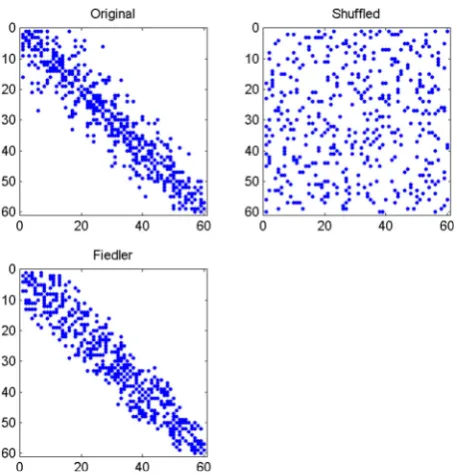
Fig. 1.Upper left: nonzero pattern in the adjacency matrix of an instance of an undirected range-dependent random graph, with two-sum of 16 518. Upper right: an arbitrarily shuffled version of this matrix, with two-sum of 269 646. Lower left: reordering of this matrix using the Fiedler vector, with two-sum of 13 304.

whereby all components of_v are shifted uniformly. To do this we add the constraintsv₂= 1 and_vT1= 0, where

· 2 denotes the Euclidean vector norm and 1 ∈RN is

the vector with all components equal to one. This gives

min

v∈RN_{,v2=1, v}T₁₌₀

N

i=1 N

j=1

(_vi−_vj)2_aij. (4)

This problem can be solved analytically through thegraph

Laplacian, _L:= _D−_B, where _B := 1

2(A+AT) and the diagonal matrix _D has_dii = _kbik. In the general case where the graph represented by sign(_B) is connected,_Lis symmetric positive semi-definite with a single eigenvalue equal to zero and corresponding eigenvector proportional to 1. The problem (4) is then solved by taking _v to be

theFiedler vector – the eigenvector corresponding to the

second smallest eigenvalue of _L; see [14–16] for further details. Having obtained the relaxed solution _v, we may recover a permutation_p∈ P via (1).

case is 16 518. The upper right picture shows an arbitrar-ily shuffled version of this matrix; rows and columns have undergone a common reordering with a permutation vec-tor chosen unformly at random. In MATLAB notation, we have _A(p,p), where_{p = randperm(60)}. This picture illustrates the type of data that we would see if we were given nodes in arbitrary order, with no information about the underlying range-dependency structure. In this case the two-sum has increased dramatically to 269 646. The lower left picture shows the effect of reordering with the Fiedler vector. Visually, we have reconstructed the concen-tration effect. In fact, this reordering reduces the two-sum to 13 304, below the level of the original matrix. We see that the Fiedler vector can be a powerful tool for uncov-ering hidden structure of this type.

In [18] a reordering approach was introduced based on the concept of the directedone-sum

N

i=1 N

j=1

(_i−_j)_aij. (5)

Here, an edge connecting nodes _i and _j makes a large positive contribution to the sum if _{i j}; that is, if the adjacency matrix entry resides far into the lower triangle. Similarly, for_ij, where the entry is far into the upper triangle, we have a large negative contribution to the sum. So, in order to emphasize any inherent asymmetry, it is reasonable to introduce the minimization problem

min

p∈P N

i=1 N

j=1

(_pi−_pj)_aij. (6)

In solving this problem, we are attempting to concentrate nonzeros in the upper right-hand corner of the adjacency matrix, and in particular, to force nonzeros into the up-per triangle. Whereas the two-sum minimization (3) was relaxed into (4) in order to produce a tractable prob-lem, the one-sum version (6) is easily solved in its dis-crete form. A solution is given by the permutation (1) induced by the “in-degree minus out-degree” vector _v = degin −degout [18], (see also Sect. 4 for a more general case). Loosely, this reordering makes the adjacency matrix appear as upper triangular as possible, and hence reveals inherent asymmetry in the network.

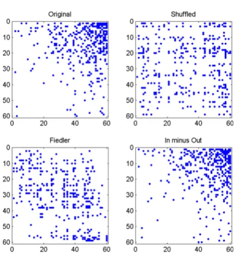
This reordering approach is illustrated in Figure 2. In the upper left picture, we show the adjacency matrix for an instance of the directed range-dependent graph model introduced in [18], where a directed edge from node_i to

j is generated with an independent probability that de-pends on _i−_j. In our case, we used the functional form 0_.95i−j+N. We see that the resulting adjacency matrix has nonzeros concentrated in its upper right corner. In this case the one-sum is −8 900, the two-sum is 365 908 and there are 30 entries in the lower triangle. The upper right picture of Figure2 shows the effect of an arbitrary node shuffle. Here, the one-sum is−1 971, the two-sum is 210 305 and 130 entries lie below the diagonal. In the lower left picture, we show the Fiedler vector reordering. It is intuitively clear that this reordering is trying to bring ele-ments closer to the diagonal. We have a one-sum of−429,

Fig. 2.Upper left: nonzero pattern in the adjacency matrix of an instance of a directed range-dependent random graph, with one-sum of −8 900, two-sum of 365 908 and 30 entries below the diagonal. Upper right: an arbitrarily shuffled version of this matrix, with one-sum of−1971, two-sum of 210 305 and 130 en-tries below the diagonal. Lower left: reordering of this matrix using the Fiedler vector, with one-sum of −429, two-sum of 98 687 and 152 entries below the diagonal. Lower right: re-ordering of this matrix using in-degree minus out-degree, with one-sum of −9 357, two-sum of 384 333 and 26 entries below the diagonal.

a two-sum of 98 687 and 152 nonzeros below the diago-nal. Fiedler reordering has reduced the two-sum, but has not revealed the inherent asymmetry. In the lower right picture, we show the “in minus out” reordering, which solves (6). In this case, we see that nonzeros are moved up and to the right. The two-sum has increased to 384 333, showing that this reordering is not trying to put similarly connected nodes together. But the one-sum is reduced to

−9 357 and just 26 entries lie below the diagonal. Hence, this ordering has revealed the inherent hierarchical struc-ture, and indeed has improved on the original ordering in terms of these two concrete measures.

3 Dynamic communicabilty

to _j, where a walk of length _w is downweighted by the factor_αw. Here _α∈(0_,1) is a free parameter whose role is to reduce the influence of longer walks. When there is only one time point, this measure reduces to the classical Katz centrality [20], and the pairwise summaries can be computed through the matrix resolvent (_I−_αA)−1. This expression can be understood from the basic linear algebra fact that the matrix power entry

(_Aw)_ij

gives a count of the number of walks from _i to _j us-ing_wedges. Generalizing to an ordered sequence of time points, [19] arrived at a product of resolvents

Q=

I−αA[0] −1

I−αA[1] −1

. . .

I−αA[M] −1

.

(7) Here,Q_ij measures how well node _ican broadcast infor-mation to node_jby forming a weighted sum of all dynamic walks that start at _i and finish at_j, with walks using _w edges downweighted by a factor_αw. To understand how

Qarises, we note that, for example,

– A[0]A[2]A[4]_ij counts the number of walks from _i to

j using one edge in time window 0, one edge in time window 2 and one edge in time window 4; and

– (_A[5])2_A[7]

ij counts the number of walks fromitoj

using two edges in time window 5 and one edge in time window 7.

The ordered product of resolvents in (7) captures all such terms – the key feature is the nondecreasing set of time indices. Just as in the original Katz version, thedynamic

communicability matrix Qinvolves a parameter,_α. In

or-der for the matrix inverses to exist, we impose the condi-tion that_αis below

α:= min

0≤k≤M

ρ

A[k] −1

, (8)

where_ρ(·) denotes the spectral radius.

Because matrix multiplication is not commutative, the dynamic communicability matrixQ depends on the time ordering of the adjacency matrices. Also, even when each

A[k] is symmetric, the resulting summary Q will be un-symmetric in general, reflecting the directional nature of time’s arrow.

We also note that products of temporal adjacency ma-trices were used later in [21] for the weaker concept of

accessibility (the existence of at least one dynamic walk

that uses at most one edge per time step).

4 Dynamic asymmetry

Our aim is now to show that the concepts in Sections 2

and 3 can be extended to provide a method for quan-tifying and visualizing dynamic asymmetry. To motivate this task, we note that there are a number of on-line and off-line circumstances where dynamic, pairwise human in-teractions have been observed to take place within a hi-erarchical structure. For example, in the context of online

forums, Graham and Wright [22] empirically investigated three types of superparticipants. One type was

agenda-setters; participants who are responsible for new thread

creation, and thereby exert a disproportionate influence

onsubsequent interactions. Quoting from [22]: “the

inclu-sion of agenda-setting reflects our view that influence is not limited to the volume of posts alone.” In an empirical study of small teams tackling simulated logistics tasks, Duchon and Patterson [23] looked for emergent thought

leaders; that is, individuals who have not been assigned

to a leadership position, but emerge over time as domi-nant in power, decision-making, and communications with respect to a particular topic. Huffaker et al. [24] studied the use of chat features between players in a Massive Mul-tiplayer Online (MMO) role-playing game, and found that in general “players send messages to higher-level experts.” We point out three common features of these examples:

– there is an inherent node ordering that is either explicit (e.g., status within an on-line game) or implicit (e.g., perceived level of expertise);

– the asymmetry manifests itself not through single peer-to-peer communication but through longer threads of interactions, where knock-on effects are at play;

– to keep track of such threads we must respect the tem-poral nature of the interactions.

A tool for quantifying and visualizing dynamic asymmetry will therefore allow us to

– discover hidden structure and track its evolution through time: for example, who are currently the key thought leaders in a particular on-line social community?

– monitor the performance of the network players within an imposed hierarchy: for example, given the manage-rial structure in a company, are any employees punch-ing above or below their weight?

– compare the inherent level of hierarchy in different so-cial networks.

To summarize how our new algorithm works, we note that the dynamic communicability matrix Q in (7) defines a single weighted, unsymmetric network that represents the pairwise ability of nodes to exchange information using the time-ordered edge sequence. Having constructedQfor the dynamic data, we may then use a generalization of the network reordering approach described in Section2in order to quantify and visualize the asymmetry.

To explain this idea in more detail, we first note that in order to avoid numerical overflow, it is preferable to work with a normalized version of the dynamic communicability matrix. We will therefore compute

Q:= Q

Q,

where·denotes the Euclidean matrix norm. To do this, we set

Q[0]_{=I (9)}

and, for each new time point_tk, form

and then reset

Q[k]_→ Q[k]

Q[k]. (11)

The final matrix

Q[M]_{=:Q (12)}

is then our overall summary. Normalizing all entries inQ by the same scalar value is not an issue since we are only concerned with their relative sizes.

To reveal the asymmetry in this dynamic network sum-mary, we may then exploit the observation that the op-timization problem (6) and its exact solution continue to make sense when we have directed and weighted edges, even allowing for negative values. We make this precise as follows.

Result.Given any_B∈RN×N the problem

min

p∈P N

i=1 N

j=1

(_pi−_pj)_bij

is solved by taking_pto be the ordering induced in (1) by the vector

v=_Bcoli−_Browi, where

Browi:=

N

j=1

bij and _Bcoli:=

N

j=1 bji

are the row and column sums of_B, respectively.

Proof.The sum

N

i=1 N

j=1

(_pi−_pj)_bij

may be manipulated straightforwardly into the form

N

i=1

pi[Browi−Bcoli].

The result then follows immediately.

In summary, having computed the normalized dynamic communicability matrixQfrom (9)–(12), we then reorder this matrix using the result above with _B =Q. By con-struction, this reordering forces large (i.e., more positive) values of Q into the top right corner. In the language of [19] we are ordering nodes according to the difference between theirbroadcast andreceive centralities.

We first illustrate this idea on a synthetic data set where the results can be interpreted clearly. We take

N = 31 nodes and allow edges to evolve according to a temporal, directed binary tree, with some added noise; in a similar way to the test in [25]. We cycle with period four across 16 time windows:

– at time windows 1_,5_,9_,13, a directed edge is inserted from node 1→2 and 1→3;

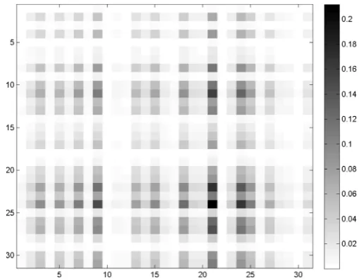
Fig. 3. Heat map showing entries in the dynamic communi-cability matrix for a binary tree cascade. Here the nodes are ordered according to the aggregate number of directed edges that they have produced. Because this ordering does not take account of the temporal hierarchy, there is no evidence of asym-metry. The one-sum for this ordering is 39.1.

– at time windows 2_,6_,10_,14, a directed edge is inserted from node 2→4, 2→5, 3→6 and 3→7;

– at time windows 3_,7_,11_,15, a directed edge is inserted from node 4→8, 4→9 up to 7→14, 7→15;

– at time windows 4_,8_,12_,16, a directed edge is inserted from node 8→17, 8→18 up to 15→30, 15→31.

In this structure nodes 1 to 15 have the same level of ac-tivity, in terms of aggregate out degree. However, there is a built-in cascade of walks down the directed binary tree. From a message passing perspective, we may view this structure as arising from a hierarchy between the nodes: there is a chain of command such that nodes pass infor-mation to lower-level individuals. To disrupt this structure slightly, we also add some noise: at each time window any other edge has an independent probability 1_/Nof arising. So we expect one unstructured directed edge per node per time window.

Taking the Katz parameter_αto be 90% of the upper limit _α in (8), Figure 3 shows the entries of Q using a gray-scale heatmap. Here, we have ordered the nodes ac-cording to their overall activity, that is, the aggregate out degree. We see that ordering with respect to this measure does not uncover the temporal pattern of information flow. The one-sum ofQ in this ordering is 39.1.

In Figure 4 we show the result from in-minus-out re-ordering. Comparing with Figure3, we see that the hier-archical structure has been highlighted, as quantified by the one-sum ofQ being reduced to−199_.4_.

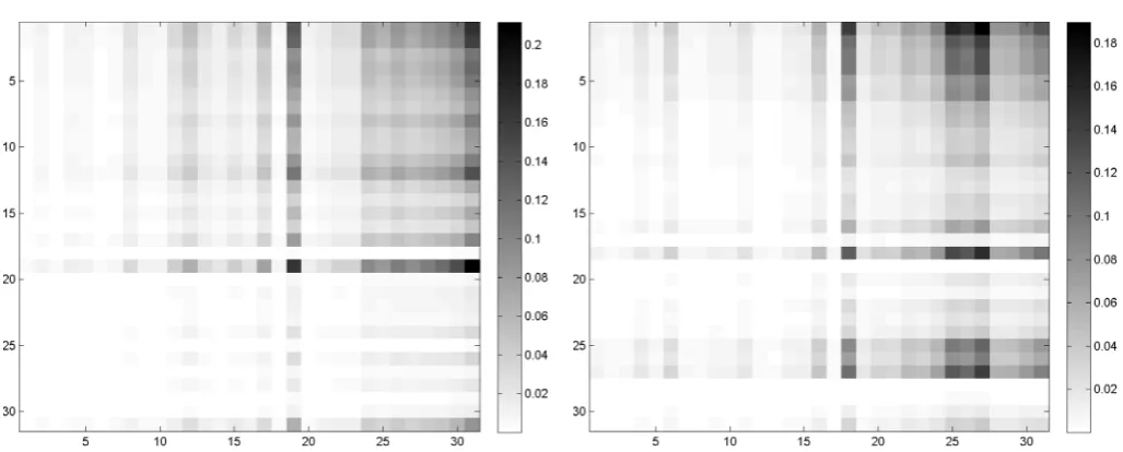
Fig. 4.As for Figure3, but with the nodes ordered according to the difference between the row and column sums of the dynamic communicability matrix. The hierarchy caused by the temporal flow of edges is now apparent. The one-sum for this ordering is−199.4.

Fig. 5. As for Figure 3, but with the time points arbitraily shuffled to dilute the cascade effect. The one-sum for this or-dering is 27.2.

likely to be reduced and it is of interest to quantify how much asymmetry remains. Ordering on aggregate activity is uniformative again, in this case giving a one-sum of 27.2. Figure6shows the result of “broadcast minus receive” or-dering onQ. Because the directed flow of information has been diluted, the algorithm reveals a reduction in the vi-sual evidence of asymmetry, as reflected in the one-sum of−171.9.

We next give results on voice call interactions from the IEEE VAST 2008 Challenge [26]. This synthetically generated set was designed to reflect interactions between members of a socio-political movement. We are given

time-Fig. 6. As for Figure4, but with the time points arbitraily shuffled to dilute the cascade effect. The one-sum for this or-dering is−171.9.

Fig. 7.Number of directed network edges (voice call interac-tions) in each 30 min time window.

stamped information for 400 cell phone users over a ten day period. There are 9 834 calls, with IDs for the send and receive nodes, a start time in hours/minutes and a duration in seconds. For our experiment, we discretized into 30 min time windows, so the directed adjacency ma-trix_A[k] is such that (_A[k])_ij= 1 when ID number_i initi-ated a phone conversation with ID number_jat least once in that 30 min period.

In Figure7, we show the number of calls in each time window. There is a clear 24 h period in the activity.

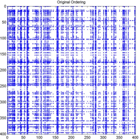
Fig. 8.Dominant entries in the normalized dynamic commu-nicability matrixQin its original ordering. Dots denote entries that are greater than the overall mean. The one-sum for this ordering is 1750.9.

Fig. 9.Dominant entries in the normalized dynamic commu-nicability matrixQwith node ordering determined by in minus out degree. Dots denote entries that are greater than the over-all mean. The one-sum for this ordering is−9 547.7.

asymmetric, in the sense that

Q = 1 and Q − QT= 0_.9968_.

In Figure 9 we show the result of the “broadcast minus receive” reordering exercise, again marking entries that

Fig. 10. As in Figure 9, but with all voice call interactions regarded as undirected. Dominant entries in the normalized dynamic communicability matrixQ with node ordering deter-mined by in minus out degree. Dots denote entries that are greater than the overall mean. The one-sum for this ordering is−4 543.2.

exceed the overall mean. The one-sum of this reordered version ofQis−9 547.7, in contrast with the value 1 750.9 arising from the original ordering in Figure8.

In Figure 10 we repeat the computations leading to Figure 9, except that voice call interactions are regarded as undirected. So each_A[k] is such that (_A[k])_ij = 1 and (_A[k])_ji= 1 when_iengaged in a phone conversation with

j at least once in that 30 min period, independently of who initiated the call. While the directed edge construc-tion used above retains informaconstruc-tion about the “chain of command,” it can be argued that this undirected alter-native is more relevant when we are concerned about the possible flow of information. We see in Figure10that there remains a visually striking asymmetry – since each_A[k] is now symmetric, this feature of the dynamic communica-bility matrixQarises solely from the time-ordering of the interactions. The one-sum for the broadcast minus receive ordering is−4 543.2 and we now have

Q = 1 and Q − QT= 0_.9995_.

5 Discussion

via their propensity to exchange information through dy-namic links. Alternative methods for extracting informa-tion may of course be derived, depending on what features are deemed important. Such choices of emphasis are essen-tially a modelling issue. We note that one particular choice is whether to respect the arrow of time. For example, the recent work [27] is aimed at quantifying network centrality based on asupra-centrality matrix of the form

M=

⎡ ⎢ ⎢ ⎢ ⎢ ⎢ ⎣

M[1] I 0 _{. . .}

I M[2] I . ..

0 _{I M}[3] . ..

..

. . .. . .. . ..

⎤ ⎥ ⎥ ⎥ ⎥ ⎥ ⎦.

(13)

Here,_M[k]is an_N by_N centrality matrix that is relevant to time_kand _I is the_N by_N identity. The authors use the simple choice _M[k] ≡_A[k] to illustrate the idea. The parameter is included to account for the fact that the identity matrices represent “between layer” connections (generally linking node_iat time_kto node_iat times_k−1 and _k+ 1) which are inherently different to the “within layer” weights arising from the network data. The key idea in [27] is to apply a standard static network centrality algorithm to the supra-centrality matrix (13). However, we note that if the individual network slices are undirected, then with _M[k] ≡ _A[k] (or with _M[k] ≡ (_I −_αA[k])−1 in the Katz-based setting), the supra-centrality matrixM is symmetric. It then becomes apparent that any static network algorithm applied toMmust be oblivious to the type of temporal asymmetry that we have discussed.

To see this another way, from a message-passing per-spective the use of the identity matrices in (13) serves to introduce links both backwards and forwards through time, so that combinatoric or random walk-based algo-rithms violate time’s arrow when interpreted on the larger matrix.

Overall, we believe that the work described here adds value to the current range of tools for summarisizing tem-poral networks, and we note that there are several promis-ing directions in which these ideas could be extended, in-cluding

(a) the development of an algorithm that applies over ar-bitrarily long time intervals by discarding chronologi-cally old information, based on the technique in [25]; (b) following on from (a), the study and categorization of individual nodes as they move dynamically through the nodal hierarchy;

(c) using ideas from [28], a related algorithm that uses a continuous-time network representation, thereby avoiding the need to specify time windows.

DJH acknowledges support from a Royal Society Wolfson Award and an EPSRC/Digital Economy Fellowship ref. EP/ M00158X/1. AVM was supported by the EPSRC and Stipso (Edinburgh) via an Impact Acceleration Account secondment ref. EP/K503861/1.

References

1. M.E.J. Newman, Networks: An Introduction (Oxford University Press, 2010)

2. L.d.F. Costa, F.A. Rodrigues, G. Travieso, P.R.V. Boas, Adv. Phys.56, 167 (2007)

3. S. Fortunato, Phys. Rep.486, 75 (2010)

4. M. Girvan, M.E. Newman, Proc. Natl. Acad. Sci.99, 7821 (2002)

5. P. Holme, F. Liljeros, C.R. Edling, B.J. Kim, Phys. Rev. E

68, 056107 (2003)

6. A.V. Mantzaris, EPJ Data Sci.3, 26 (2014)

7. M.P. Rombach, M.A. Porter, J.H. Fowler, P.J. Mucha, SIAM J. Appl. Math.74, 167 (2014)

8. M.A. Riolo, M.E.J. Newman, J. Complex Netw. 2, 121 (2014)

9. O. Sporns, R. Kotter, Plos Biol.2, 1910 (2004)

10. G.H. Golub, C.V. Loan, Matrix Computations, 4th edn. (Johns Hopkins University Press, 2012)

11. T.A. Davis, Direct Methods for Sparse Linear Systems (Fundamentals of Algorithms 2) (Society for Industrial and Applied Mathematics, Philadelphia, 2006)

12. S.T. Barnard, A. Pothen, H.D. Simon, Numerical Linear Algebra2, 317 (1995)

13. D.J. Higham, J. Comput. Appl. Math.158, 61 (2003) 14. F. Chung, Spectral Graph Theory (American

Mathema-tical Society, Providence, 1997)

15. G. Strang, Computational Science and Engineering (Wellesley-Cambridge Press, 2008)

16. R. Van Driessche, D. Roose, Parallel Comput. 21, 29 (1995)

17. P. Grindrod, Phys. Rev. E66, 066702 (2002)

18. J.J. Crofts, D.J. Higham, Internet Math.7, 233 (2011) 19. P. Grindrod, D.J. Higham, M.C. Parsons, E. Estrada,

Phys. Rev. E83, 046120 (2011) 20. L. Katz, Psychometrika18, 39 (1953)

21. H.H.K. Lentz, T. Selhorst, I.M. Sokolov, Phys. Rev. Lett.

110, 118701 (2013)

22. T. Graham, S. Wright, J. Comput. Mediated Commun.

19, 625 (2014)

23. A. Duchon, E.S. Patterson, in Social Computing, Behavioral-Cultural Modeling and Prediction (Springer, 2014), pp. 51–58

24. D. Huffaker, J. Wang, J. Treem, M. Ahmad, L. Fullerton, D. Williams, M. Poole, N. Contractor, IEEE Int. Conf. Comput. Sci. Eng.4, 326 (2009)

25. P. Grindrod, D.J. Higham, SIAM Rev.55, 118 (20013) 26. G.G. Grinstein, C. Plaisant, S.J. Laskowski, T. O’Connell,

J. Scholtz, M.A. Whiting, VAST 2008 Challenge: Introducing mini-challenges, in IEEE VAST (2008), pp. 195–196

27. D. Taylor, S.A. Myers, A. Clauset, M.A. Porter, P.J. Mucha,arXiv:1507.01266 (2015)

28. P. Grindrod, D.J. Higham, A dynamical systems view of network centrality, Proc. R. Soc. A470, 20130835 (2014)