Visual cavity analysis in molecular simulations

City, University of London Institutional Repository

Citation:

Parulek, J., Turkay, C., Reuter, N. and Viola, I. (2013). Visual cavity analysis in

molecular simulations. BMC Bioinformatics, 14(19), pp. 1-15. doi:

10.1186/1471-2105-14-S19-S4

This is the unspecified version of the paper.

This version of the publication may differ from the final published

version.

Permanent repository link:

http://openaccess.city.ac.uk/3614/

Link to published version:

http://dx.doi.org/10.1186/1471-2105-14-S19-S4

Copyright and reuse: City Research Online aims to make research

outputs of City, University of London available to a wider audience.

Copyright and Moral Rights remain with the author(s) and/or copyright

holders. URLs from City Research Online may be freely distributed and

linked to.

R E S E A R C H

Open Access

Visual cavity analysis in molecular simulations

Julius Parulek

, Cagatay Turkay

, Nathalie Reuter

, Ivan Viola

From

2nd IEEE Symposium on Biological Data Visualization

Seattle, WA, USA. 14-15 October 2012

Abstract

Molecular surfaces provide a useful mean for analyzing interactions between biomolecules; such as identification and characterization of ligand binding sites to a host macromolecule. We present a novel technique, which extracts potential binding sites, represented by cavities, and characterize them by 3Dgraphs and by amino acids. The binding sites are extracted using an implicit function sampling and graph algorithms. We propose an advanced cavity exploration technique based on the graph parameters and associated amino acids. Additionally, we interactively visualize the graphs in the context of the molecular surface. We apply our method to the analysis of MD simulations of Proteinase 3, where we verify the previously described cavities and suggest a new potential cavity to be studied.

Introduction

Molecular biology is studying biological phenomena on the highest magnification level where the life processes are carried out by interactions of molecular machinery. One key focus of this scientific branch is to study and deter-mine the molecular structure, while another attention is given to its dynamics and interactions with the other molecules. The structure, or conformation, of a protein can for example be obtained through the crystallography and the interactions of the protein with its environment are modeled by means of Newtonian physics, involving potential energy, where induced forces modify the struc-tural arrangement of the molecule. They are often referred to as molecular dynamics (MD) simulations. The outcome of the simulation is then stored as a sequence of transfor-mations for each atom of the molecule or environment, denoted as trajectories.

The studied macromolecules such as proteins are typi-cally analyzed for a binding site to act as a carrier of an important chemical substance. Alternatively, a small mole-cule is searched for that would change the conformation of a particular protein and by the structural change influ-ence a certain chain of molecular interactions, called as pathways. For example in a pathway of a certain cancer types, one would like to change the conformation or to

block the binding site of a participating protein to disable a successful execution of the pathway.

Typical questions raised by molecular biologist in their exploratory workflows are where is a suitable binding site, what are its chemical characteristics and how stable this binding site is over the simulated time. Typical car-riers and binding sites are channels, pockets, and cav-ities on the molecular surface.

One way of channel and pocket detection and analysis is to perform the Monte Carlo sampling over the bound-ary of the macromolecule. Cavities can be identified and characterized by means of differential geometry on the molecular surface [1,2]. These techniques are mostly quantitative and non-visual.

Parallel to these approaches are analytical methodologies that utilize visualization of the molecular surface where the biologist assesses the molecular structure qualitatively and searches for potential binding sites. For this type of analysis it is very important that shape and depth cues are effectively communicated to the viewer [3].

We have identified the importance of the complemen-tarity of these two approaches and propose a novel visual analytics framework for the cavity analysis. The cavity candidates are extracted automatically from the molecu-lar structure for each timestep of the simulation. After the extraction process the user can visually analyze the cavity geometry, chemical properties and other important quantitative measures. The user can formulate a query

* Correspondence: [email protected]

1_{Department of Informatics, University of Bergen, Norway}

Full list of author information is available at the end of the article

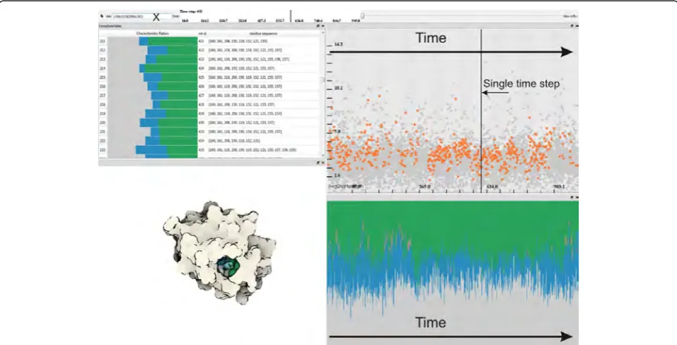
for finding cavities that correspond to particular envi-sioned characteristics and by interacting with the tem-poral settings she can quickly get familiar with the binding site stability over time (Figure 1).

It is noteworthy that this work represents a natural continuation of our previous study [4], which focused mostly on the graph based cavity representation. Here we extend this technique by an improvement of the implicit function sampling and the 3Dvisualization, and also by characterization of the graph components by amino acid types.

Related work

Our work can be regarded as related to two groups of techniques, namely implicit molecular representation, and cavity extraction.

Implicit molecular representation

In order to model complex and dynamic geometric objects, implicit surfaces are a suitable mechanism. In the molecular visualization field, implicit representation has been used widely to smoothly model the bond tran-sitions between single atoms. Blinn [5] used the set of techniques for the first time, which are today known as implicit modeling. In order to describe the electron

density function of the atoms, he utilized an implicit function that sums up the contribution from the atoms:

f(p) =T− i

bie−aid

2

i_,

(1)

withdias the distance frompto the center of atomi,

bias the “blobbiness”, aias the radius of the atom, and

Tas a threshold for the electron density. In later studies, implicit surfaces that are constructed from skeleton points were introduced [6,7]. In general, these represen-tations can be formulated as:

f(p) =T− i

mifi(p), ₍₂₎

wheremiis a weight factor andfi is a density distribu-tion funcdistribu-tion that is decreasing. Shestyuk [8] presented a comparative analysis on how different distribution functions can be applied. The performance of the kernel evaluation in the rendering process was improved by GPU implementations [9], which were later used for fast visualization of molecular surfaces [10,11]. The above approaches that use the summation of atom contributions can be considered to be relatively fast and thus widely used. However, these approaches do not completely

consider the solvent that is usually represented as a sphere with radiusR. The consideration of the solvent, on the other hand, can lead to valuable findings that can lead to potential binding sites.

Pasko et al. [12] combined different implicit model forms to propose a generalized implicit surface repre-sentation. The implicit object representation is denoted as a function that involves the following inequality:

f(p)≥0, (3)

wherep= (x1, x2, x3)Î E3andfis an implicit surface

function (or implicit function). fclassifies the space into two half-spaces:f(p)>0 andf(p)<0. The above classifi-cation is also valid for Eqs. 1 and 2.

There are a number of methods to represent molecular surfaces. A common approach is to represent atoms as spheres with radii that amounts to the van der Waals forces (vdW surface) [13]. The implicit function for the van der Waals that follows Eq. 3 is defined as: f(p) =∪i(ri−di), whereriis the van der Waals radii. By extending the sur-face with a solvent radius, one obtains a solvent accessible surface: f(p) =∪i((ri+R)−di).

In the cavity exploration area, the most common representation is the solvent excluded surface(SES) [14]. Recently, Lindow et al. [15] and Krone et al. [16] pro-posed GPU implementation of the SES representation. Although they achieved a high rendering performance, their models are solely applicable to rendering related tasks. Our cavity detection method, introduced in this work, requires that the molecule is defined as an impli-cit surface.

Parulek and Viola [17] introduced a functional represen-tation for the modeling and the visualization of theSES

representation. In their method, the molecular surface is represented as a combination of basicCSGoperators and they define a distance based implicit function. Our func-tion sampling procedure uses this representafunc-tion as a basis. Further details are in the Visualization section.

One method to visualize implicit molecular models is to construct a mesh representation and render the mesh as a set of patches [18]. However, in the case of complex molecules the resulting meshes can consist of millions of triangles, which creates a challenge to generate detailed iso-surfaces. As a result, direct visualization techniques such as ray-casting have been introduced recently.

One subclass of implicit surfaces are represented by distance based functions. Effective visualization of such objects was proposed by Hart [19]. Since, essentially, the distance measure for an implicit function can be approxi-mated by the first Newton iteration of the function:

fdist(p)≈ f(p)

|∇F(p)|; (4)

we also adopted Hart’s technique for rendering.

Analysis of protein cavities

Since the empty spaces on protein surfaces provide valu-able information, they have been investigated widely in the literature. Many methods utilize the analytical description of theSES[20]. For instance, Voss and Gerstein [21] intro-duced a web-based cavity analysis tool that apply two separate probes to calculate the solvent volume to search for potential cavities and channels.

There are also several tunnel exploration methods. In general, these methods require the specification of an initial point in the empty space within the protein. The method tries to reach the exterior by following tunnel-like cavities and fills the space with geometric structures as it progresses. These methods also provide information related to the pathway around the exit area to describe the cavities. The method HOLE [22], uses a similar strategy, where the user defines the initial location and orientation of a pore within the molecule. The specification of the initial parameters have been automated by Coleman and Sharp [1], where their algorithm is also capable of deter-mining arbitrarily shaped tunnels. Voronoi diagrams have been used to discover molecular channels and pores in CAVER [23] and MOLE [24]. Recently, Voronoi diagram of spheres showed its potential to extract significant paths from the molecules [25]. Random rays are generated at Voronoi vertices in order to remove them outside the molecule. Although the use of ray casting to determine cavities is similar to our method, we utilize an implicit function sampling rather than Voronoi vertices. Our method puts more emphasis on the molecular surface.

Pore features are utilized to determine channels in an iterative and heuristic algorithm in Pore-walker [26]. Within the context of tunnel extraction methods, our approach can be described as a combination of stochas-tic methods due to use of function sampling, and Voro-noi diagrams due to use of graph analysis.

Molecular pockets and cavities have also been subject to many studies. CAST uses computational geometry together with alpha shape theory in order to extract cav-ities [27]. Till and Ullmann use a Monte Carlo algorithm while sampling a protein surface over a 3D grid [2]. Although the use of randomly sampled points to calcu-late cavities is similar to our method, we directly use the sample points to estimate the cavities rather than using a 3Dregular grid. Moreover, our approach also includes the use of interactive visual analysis to investigate the resulting cavities.

Instead, we present a set of potential cavities for each time step, where the user has the functionality to explore this set of cavities through linked views and interaction.

Method overview

To represent molecular surfaces by an implicit function

f(p), we employ the approach introduced by Parulek and Viola [17]. Nevertheless, one can use a kernel based approach (Eq. 2), and as well as vdW or SAS, which both can be easily expressed as implicit functions. The implicit function is positive inside the molecule and negative outside, and it is possible to estimate the mini-mum distance of a sample point from the surface. The distance can be computed by the application of New-ton’s formula, (Eq. 4).

Similarly to our former study [4], we compute an independent set of graphs,Gt ={Gt₁∪. . .∪Gtm}, repre-senting m cavities of MD simulation in time step t

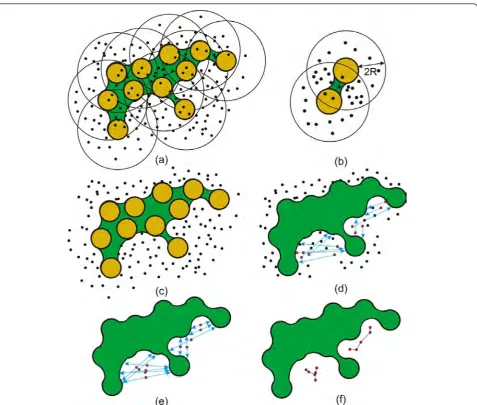
(Figure 2). Here we improve the positioning of sample points forming the graphs. These samples are generated with respect to atom centers within radius [ri,ri + 2R] from each atom, i.e., within the influence of the atom. Moreover, for each cavity graphGt_i, we compute graph parameters, e.g., the average shortest path, and amino acids that compose the molecular surface near the graph. The user is provided with the system of linked views allowing her to select individual graphs according to the graph parameters and as well as by direct amino acids specification.

Cavity graphs

In the first stage, we sample the implicit functions by a set of random points, S = {p1, ..., pn}, which densely

cover the function domain (Figure 2a). One of the important issues related to cavity extraction from the molecular implicit function is how to prefer regions with higher surface complexity. This is due to the fact that the occurrence of the cavities is directly related to the surface complexity. In another words, we should emphasize surface regions with a higher curvature varia-tion. Fortunately, this is highly correlated with respect to the density of atoms in that region, since the function evaluation employs the closest atoms only, i.e., within distanceri+ 2Rfrom thei-th atom. Therefore, the sam-pling can be performed by generating an equal number of sample points for each atom, which will naturally cre-ate more sample points in regions with more atoms, i.e., in regions with higher surface variations (Figure 2b). We perform the sampling for every time step of the MD simulation, where the positions of sampling points remain almost the same for all the time steps, i.e.; we slightly adjust the position with respect to the molecular bounding box in a particular time step.

The sampling process evaluates the implicit functionf

at every sample position; i.e., we obtain a set of function values Ft = {f(p1), ..., f(pn)} for time step t, where

n represents the number of samples. With respect to the property of implicit functions that classifies points between internal and external ones, we can easily filter out samples S0 ⊆ S that lie inside the protein,

S0 = {p|f(p)≤ 0;pÎS} (Figure 2c), which do not belong

to any cavity.

Essentially,S0contains a set of sample points lying in

a close vicinity of the surface, up to a distance of maxi-mum 2R from the molecular surface, which is clear from the sample point definition.

As a next step, we perform a cavity based analysis, which classifies the samples into potential cavity sam-ples. Note that there is no exact cavity definition with respect to any of aforementioned molecular surface defi-nitions, i.e., van der Walls spheres, solvent accessible surface, solvent excluded surface, blobby models, etc. Nevertheless, there are at least some hints on how the cavity can be described. In our work we follow the spe-cification by Cheng and Shi [29], which describes a cav-ity as a connected and concave surface patch that might open up to the outside via a narrow mouth. This prop-erty allows to define the cavity through opposite facing surfaces. This condition is verified at each sample by a ray that is cast along the normal direction beginning at the sample. In a case that the ray hits the surface, the sample is classified as a potential cavity sample [4] (Figure 2d). Thus only the samples that lie between two opposite facing surfaces are labeled as a potential cavity. Although this excludes more shallow regions, it was still preferred and recommended by our collaborators from bioinformatics. On the other hand, the ray-casting method can be performed in a more robust way, such as for instance producing multiple rays in various direc-tions. Nevertheless, casting just a single ray is a very fast method and, when taking into account the large number of employed samples, it also filter out many false posi-tives in the set S0. Afterwards, we adjust the sample

position to lie in the middle of two opposite facing sur-faces (Figure 2e).

The number of points (samples) that are seeded to the spatial domain depends primarily on the size of the molecule: for instance for Proteinase 3 (3346 atoms), used in our use case, we employed 16 samples per atom, i.e, 3346 × 16 = 53536 of sample points. The number is significantly lower than in approaches that employ regular grid discretization, e.g., 2563

extracted cavities does not change dramatically, this number defines the amount of required samples.

In the next stage, our goal is to form a graph that defines the relations between the cavity samples. First, we perform visibility tests between all pairs of sample points. This generates an undirected graphG, where nodes are the sample points and edges are mutually visible samples. Secondly, we perform the connected component analysis, which results into the set ofmindependent subgraphs

G= {G1∪...∪Gm}. Thirdly, we apply a minimum span-ning tree algorithm [30] to each componentGito build its central skeleton (Figure 2f).

For more details on our graph extraction technique, we refer readers to our previous study [4].

Visualization

The rendering of implicit surfaces representing molecules by a single distance based function was introduced by Parulek and Viola [17]. In our previous study, we improved the proposed pipeline by utilizing spherical impostors representing an area of the atom influence [4].

To ease the shape perception, we farther improve the surface rendering by contour enhancement. In the litera-ture, there are several papers on contour enhancement

techniques [31]. The simplest one employs the angle between the surface normal and the viewing direction. The disadvantage is that flat boundary regions that have similar gradients may become a part of the contour as well. Therefore we turn to curvature-based techniques, which can suppress contours in low-curvature regions. On the other hand, those techniques are usually compu-tationally demanding. Therefore, we adopt a technique introduced by Bruckner and Gröller [32], which approxi-mates the view-dependent curvature by evaluation of two consequential gradients along the viewing ray. Moreover, it easily allows to change contour thickness (Figure 3 middle and right).

The surface color is determined by the amino acid type. The amino acids are the basic building compounds of molecules, and also provide a deeper relation for biol-ogists with our cavity analysis. We classify the amino acids into four categories, according to the classical amino acid Venn diagram [33]. The four categories of amino acids are hydrophobic (white), negatively charged (red), positively charged (blue) and polar ones (green). The final surface color is determined by the closest amino acid with respect to the surface point.

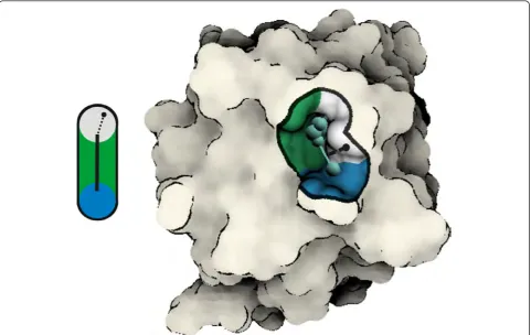
To allow for molecule exploration, we include a clip-ping plane interaction, which we refer to as an implicit clipping plane (ICP). The ICP clips away the atoms from the implicit surface. This enables us to study even occluded cavities located inside the molecule. Here we exploit the fact that the implicit function is constructed on the fly during the ray-casting. The ICP neglects those atoms that lie in front of the clipping plane (Figure 3 left). The reason for using such a clipping plane is to pre-serve the molecular surface in the close vicinity of the

plane. Users can either link the plane normal with the viewing direction, or adjust the plane orientation interac-tively. Additionally, when the implicit clipping plane is activated, the diffuse shading model is evaluated just for the surface area that is not clipped. This enables us to distinguish between the clipped surface and the original one. For the clipped surface points we utilize just con-stant colors derived from the amino acid type (Figure 3 middle and right).

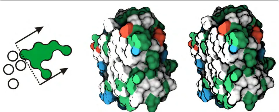
To depict the graph components, we use basic geome-trical primitives, i.e., spheres and line segments. The radii of spheres are defined by the sample distance from the molecular surface [4]. The edges represent the mini-mum spanning tree of each graph. Our system allows to select and visualize a group of graphs for each time step separately. We visualize the graph components in the focus and context style. The focus, the molecular surface close to the selected graph component, is colored using the amino acid type, whereas the context, the molecular surface farther away from the selected graph compo-nent, is shaded constantly (Figure 4).

Graph attributes

The cavity extraction procedure generates tens of graphs per time step over a simulation containing thousands of time steps. Therefore, direct integration of all the graph components into the visualization can easily produce results that are cluttered and difficult to interpret. In our former study [4], we introduced an interactive system that allows performing visual selection of the graph com-ponents to steer the focus of the cavity analysis. To ease the graph exploration, we compute a set of basic graph measures: the longest path between any two nodes, the

average length of the shortest paths between pairs of nodes (avgP), and the average of the degree of all the nodes. In our examples we employavgPfor selections, which essentially represents the overall cavity size.

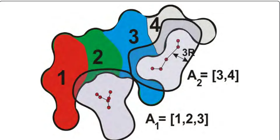
Additionally, we compute amino acids (Ai = {a1, ...,

ak}) that compose the molecular surface near the cavity graph Gi. Here, we employ the geometrical distance

Dg= 3Rfrom the cavity graph, i.e., if there is an inter-section between the molecular surface and the graph component (Figure 5), we assign the amino acids com-posing the surface to the graph. The assignment of amino acids is illustrated in Figure 5.

By utilizing the properties of the amino acids Ai (assigned to the cavity Gi), we compute a profile of the cavityGi. We build this profile by utilizing a categoriza-tion of amino acids based on their chemical properties [33], i.e., the same as we employ for the surface colors. In order to build the profile of a cavity according to these categories, we iterate through the atoms that form the molecular surface near the cavity graph (Figure 5). We mark each atom according to the type of the amino acid it belongs to, e.g., if an atom is a part of a polar

amino acid, it is considered to be polar. After all the atoms are marked, we count the number of atoms and compute the ratios for each category. We use these ratios to visually represent the profile of a cavity, where each category is mapped to a color: gray for hydrophobic, green for polar, blue for positively charged, and red for negatively charged amino acids.

Interactive analysis of graph components

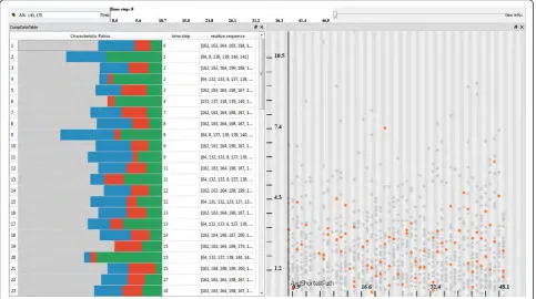
The computation of the graphs and their attributes results in heterogeneous data related to the simulation. At this stage of the analysis, we have three different types of data involved in the visualization: i) the raw simulation data ii) the graph components data iii) the amino acids data. In order to analyze these heteroge-neous data, we make use of a coordinated multiple view setup that employs interactive visual analysis (IVA) methods. Our setup employs linked views, where each type of view can handle different parts of the data. Firstly, to visualize the raw simulation data, we make use of the 3D visualization method previously discussed (Figure 1 bottom-left). Secondly, we utilize a scatterplot

Figure 4Visualization of graph components. Left: The iso-surface point (the black circle), obtained during ray-casting, is evaluated against the distance (the dashed line) to the graph component (the black line). Right: An example of graph component visualization in the context of the molecule. When a graph component is shown, the coloring is applied only to points that lie within distanceDg= 3Rfrom the graph. We

employ flat shading for surface points lying beyondDg. The boundary ofDgis shown as a black contour on the surface. The graph component

that visualizes a selected graph attribute (y-axis) over time (x-axis), where each dot represents a unique graph component (Figure 1 top-right). Finally, two separate views show the data related to the amino acids. One view visualizes the chemical properties of cavities (cavity profiles) over time (Figure 1 bottom-right) and another view lists the selected cavities and their amino acids ordered by time (Figure 1 top-left).

These different views are linked using an interaction method called linking & brushing. This method enables the user to interactively make selections (also called brushes) in one view and observe what structure the same selection corresponds to in the other views. In order to visually express the selection in the views, we make use of two methods. In the first method, we high-light the selected data in the context of the whole data. Example of this method could be seen in the graph attribute scatterplot, where the selected graphs are high-lighted by orange color and the rest of the graphs, the unselected ones, are displayed in gray (Figure 1 top-right). The second method displays only the selected information. An example of this method is the cavity profile view, where only the profiles of the selected graphs are shown (Figure 1 bottom-right).

In our system there are two different ways to select graph components. The user can either interactively select (brush) the graphs through the graph attribute scatterplot (Figure 1 top-right) or specify the amino acids through textual queries. Additionally, different selections

can be combined via the basic Boolean operators (AND,

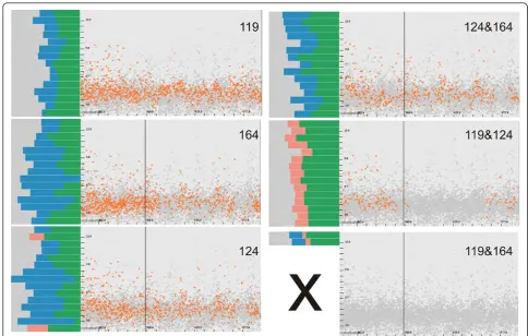
ORandNOT), which lead to more complex queries. One important point to mention is that all the views are updated automatically whenever a selection is made. For example, in the amino acid list view it is possible to select cavity graphs through a direct specification of amino acids that are of interest, and the other views display the selec-tion immediately. Through this view, the user composes textual queries that includeAND= & andOR=∨ opera-tions. In Figure 6 we specify two amino acids 140∨170, which selects graphsg= {Gi|140ÎAi∨170ÎAi;GiÎG}. In the accompanied scatter-plot we can observe the distri-bution of these graphs,g, over time. Additionally, it is pos-sible to combine queries by specifying the intervals of amino acids, e.g., the query (120−140)&(180−190)&173 represents all cavities that contain at least three amino acidsai,aj,ak, such thataiÎ[120, 140],ajÎ[180, 190] andak= 173.

Implementation and performance

We implemented the entire system in Python program-ming language, where most of the rendering and com-putations run on the GPU (CUDA and GLSL). The performance measurements are done on a workstation equipped with two 2 GHz processors and 12.0 GB RAM, and with a GPU NVIDIA GeForce GTX 680. The 3Dcavity visualization in the context of the molecular surface is performed on the fly (GLSL for sphere bill-boarding and CUDA for ray-casting). The molecular

Figure 5An illustration of the assignment of amino acids to the graph components. We turn the cavity skeleton into a distance object, bounded by the distanceDg= 3R, and perform an intersection with the molecular implicit function. We mark those atoms/amino acids that

visualization can be performed even without the cavity segmentation, since the ray-casting pipeline is indepen-dent from the graph analysis. Prior to 3Drendering and cavity segmentation, the only auxiliary structure that needs to be computed is the GPU representation of atoms.

We utilize a simple and straightforward approach that is based on an uniform spatial subdivision. This has been already utilized by the broad molecular visualiza-tion community [15,16]. The atoms are sorted into cubic voxels with a lateral length of 2radiusmax+ 2Rmax, where radiusmax represents the maximum (van der Waals) radius of all the included atoms andRmax repre-sents the maximal allowed solvent radius. Then, in order to find the closest atoms to a given point, it is required to visit 3×3 ×3 neighboring voxels. Thus, for a given time-step, we need to send to the GPU only the atom centers and their radii, and the grid of voxels. Such a grid of voxels is computed and stored automati-cally when the user selects a particular time step either to visualize or analyze, which has not been processed before.

In the process of cavity segmentation all the samples are precomputed for the entire simulation, where the user has the possibility of resampling a particular time-steps if

desired. All the samples are evaluated in parallel, time-step wise, using CUDA. For instance, evaluating and segment-ing 50Ksamples for 1000 time steps takes around 20 min-utes. After the cavity samples have been segmented, the user can initialize the computation of graph components. The generation of graphs takes around 10 minutes for 1000 time steps, for the previous example. The process of assigning amino acids to the generated graphs is automati-cally executed after the graphs have been formed. This takes approximately another 10 minutes. After these pre-processing steps are over, the system operates at interac-tive rates. It is important to mention that, even when performing complex queries constructed through our selection mechanism, the system gives an immediate response.

Use case: analysis of Proteinase 3

Proteinase 3 (PR3) belongs to the family of serine pro-teases, cleaving proteins via specific hydrolysis of peptide bonds. It is an enzyme involved in inflammation, where in a number of chronic inflammatory diseases, e.g., Wegener granulomatosis and vasculitis, PR3 has a deleterious effect. Therefore, PR3 is a drug target. To design drugs for PR3, we need first to understand of how ligands bind to it, which is conditioned by a better characterization of the

binding sites. This allows the development of drug candi-dates with higher affinity to PR3 than its endogenous targets [34].

The search for new drugs often relies on knowledge of the three-dimensional structure of the enzyme involved, and in particular of the cavities on its surface. The drug candidate efficiency is dependent on a strong interaction with the enzyme. The strong interaction can be achieved by binding into a cavity. Nevertheless, all molecules are dynamic and the structural changes they undergo impact their function. This is also valid for the dynamics of cavities. Thus our goal is to provide dynamic picture of the relevant cavities over the simulation time.

The analysis starts with importing thePDB andDCD

files for PR3. The Protein Data BankPDBfile format is the most common format for atomic cartesian coordi-nates and other relevant information (e.g., atom types, amino acid types, sequence numbers). TheDCDfile for-mat is commonly used for MD simulation trajectories, and is the output format of MD engines, such as CHARMM [35] or NAMD [36]. For demonstrational purposes, we limit the number of time step analyzed to 1000.

After loading the data, the user can already visualize the molecular surface in the 3Dview. In the context menu that is available in the application, the user can select multiple commands that run the sample and the graph components generation. Here, one can decide to execute all the computations, i.e., samples evaluation, graph creation and amino acids computation, at once for the entire simulation or for each time-step individually.

Our framework computes automatically the number of occurrences of amino acids with respect to the graphs. Using this information, one can easily find the graphs/cav-ities, which refer to the most present amino acids in the MD simulation. Moreover, throughANDandOR opera-tions and the linked 3Dview, one can verify whether those amino acids belong to the same cavity.

Another possibility is to verify a priori knowledge of the cavity that is formed by specific amino acids. Here the user can specify the corresponding amino acids queries by the ANDoperation, or by OR operation to see whether the occurrence of the selected graph com-ponents in the accompanied temporal scatter-plot has changed.

Benchmarking against known binding sites

Here we firstly show how to perform validation of exist-ing bindexist-ing sites discoveries. Hajjar et al. [34] evaluated a binding site that had been early characterized as con-taining an isoleucine (Ile171) and an aspartic acid (Asp190). The characterization originated from visuali-zation of the X-ray structure of Proteinase 3. Using MD simulations of Proteinase 3 with many different ligands

docked in the binding site, Hajjar and coworkers showed that Ile171 and Asp190 did not play any significant role in the interactions with the ligands. Instead Ser176 and Val193, as well as possibly Ser191 were interacting with most of their ligands. Additionally, there might be another cavity formed by, among others, Asp190 and Ile1.

It is important to mention that these results were obtained by a series of MD simulations, where each simula-tion represents another ligand bound to Pr3. The analysis consisted in measuring the occurrences of contacts between the ligand and any amino acid of Proteinase 3. Here we show that, with our visual analysis framework, we can directly evaluate some of these binding sites by analyz-ing just a sanalyz-ingle MD simulation. Moreover, with our method, the analyst gets an overview of the existing cavities, characterized in terms of size and chemical properties.

Val193, is likely to be composed of two distinct concave surface features that are divided by a surface extrusion. This hypothesis is supported by the amino acid query 176∨193, which shows that there are cavities formed by at least one of these amino acids (Figure 7). Such a com-pound cavity is not within the frame of our cavity description that requires the connectivity of the concave surface patch. Moreover, a difference between their and our study is that they analyze which part of PR3 interact with ligands (no cavity analysis) to derive a model of the binding sites, while we are looking at actual cavities on the molecular surface. That might explain the apparent discrepancy.

As a consequence, and as a next step, we perform sev-eral extended selections to see whether other amino acids might contribute to the cavity (Figure 9).

Unsupervised cavity discovery

Hajjar et al. investigated the so-calledS4−S1 andS1’−

S3’binding sites of Proteinase 3, and for doing so they

performed analysis of numerous MD trajectories of PR3 with ligands. The design of their simulations and subse-quent analyses were directed solely towards these binding sites and did not investigate other potential binding sites.

In the case of PR3, for which we analyzed the same MD simulation as was described in the previous section, we are able to discover cavities distinct from the known peptide binding sites; in particular one clear polar/ hydrophobic but also with Arg (positively charged amino acid). By finding this cavity we have highlighted a region of the Proteinase 3 that has potentially an impor-tant role for its function. This cavity can be further characterized by our colleagues in molecular biology, who have the possibility to design experiments to inves-tigate its potential functional role.

Since each graph component/cavity contains a list of participating amino acids, we can easily compute the most present amino acids over the entire simulation. By order-ing the amino acids by their occurrence we made a list of the four most present amino acids, and we performed

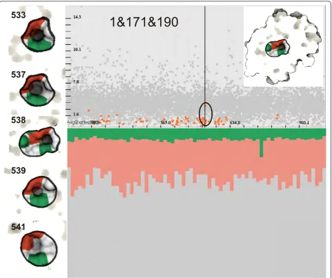
Figure 8A cavity formed by Ile1, Ile171 and Asp190 (1&171&190). Left: An illustration of of the same cavity in different time steps (533,537,538,539 and 541) marked by the black circle in the temporal scatterplot. We performed specification of 1&171&190 as a continuation of the analysis started in Figure 7, which shows that the cavity might be formed by all three amino acids. The cavity is located deep inside PR3 and we have to use the ICP to show it. Bottom-right: It is easy to see that the chemical properties of the cavity are very stable over entire simulation, where hydrophobicity prevails over polarity.

ANDoperations between all of them. These amino acids are: Val119, Val150, Thr152 and Arg208. We verify the presence of the graph components in the scatterplot (Fig-ure 10 top), and the cavity shape and its span on the

molecular surface in the 3Dview (Figure 10 bottom). Then we can continue with the analysis of the chemical properties. Additionally, we estimated that the cavity graph formed by at least Val119 is present in the

simulation for 86.5% of the total time, while all four amino acids form the cavity for 63% of the total time. We show-case this cavity in Figure 10, where we also see its chemi-cal properties over time.

Conclusions

We introduced a framework capable of detecting and visualizing cavities in molecular simulations. Furthermore the cavities are described by means of graphs, for which we compute graph attributes and a list of amino acids that constitute the molecular surface around the cavity graph. We used a brushing and linking methodology to analyze the graph attributes through dedicated views. We pro-posed a visualization method to show cavities in the con-text of the molecule. Additionally we introduced an implicit clipping plane that let us visually investigate occluded cavities localized inside the molecule.

Moreover, we have shown that our system enables to verify existing cavities through specification of amino acids of interest. We studied cavities defined by logical operators of the amino acids Ile1, Ile171, Ser176, Asp190, Ser191 and 193 in Proteinase 3 MD simulation. Additionally, we found out that there might be another cavity formed by at least four amino acids Val119, Thr152, Arg208 and Val150, which were even more per-sistent than the known ones. Our collaborators in biol-ogy agreed to study the discovered cavity more deeply.

One of the major limitations in our cavity extraction approach relates to the definition of the cavity. As already mentioned, the cavity is considered as a concave surface depression with a possible narrow opening when located on the molecular surface. To detect also shallow surface cavities, we can cast multiple rays from the sam-ple point in distinct directions. However, such an approach will produce many false positives, which still can be reduced by the accompanied linking and brush-ing mechanism. This represents our future studies.

Another task that was demanded by our collaborators from biology was to track graph components over time. This is partly solved by linking amino acid selections. Nevertheless, it might happen that more than one cavity touches the same amino acid. This can be tackled by graph matching method applied on pair-wise graph components located in neighboring time steps. Here, possible scenarios of graph developments cover mainly splitting and merging of graph components between sequential time steps.

Another challenge is represented by incorporating charges into the existing concept. Electron potential charges are usually solved on the discrete volumetric grid by means of solving PDE. Since the implicit repre-sentation evaluates the function values anyway for any point in space, both representations can be easily

merged. The resulting charges can then be mapped both to the graph components and to the iso-surface of the molecule.

List of abbreviations used

vdW: van der Waals; SAS: Solvent Accessible Surface; SES: Solvent Excluded Surface; PR3: Proteinase 3; ICP: Implicit Clipping Plane; GLSL: OpenGL Shading Language; GPU: Graphics Processing Unit; CUDA: Compute Unified Device Architecture.

Competing interests

The authors declare that they have no competing interests.

Authors’contributions

JP developed the major framework and algorithms, implemented the 3D

visualization and the 2Dviews related to amino acids. CT developed the 2D component view, implemented the brushing and linking technology, and the views for graphs components to enable the IVA process. IV brought focus and context visualization ideas. Additionally, he contributed to development of the cavity detection algorithm. NR provided the MD data, introduced the biological background and suggested to focus on amino acids, their detection algorithm, and discussed the cavity evaluation and discoveries. All authors wrote, read and approved the manuscript.

Acknowledgements

This work has been carried out within the PhysioIllustration research project (# 218023), which is funded by the Norwegian Research Council. A minor part of the project has been funded by the Vienna Science and Technology Fund (WWTF) through project VRG11-010. NR acknowledges funding from the Bergen Research Foundation, and support from the Norwegian Metacenter for Computational Science (NOTUR). We would also like to thank Helwig Hauser and Visualization group in Bergen for useful ideas and feedback. Additionally, we would like to give thanks to anonymous BioVis reviewers for their useful feedback.

Declarations

This publication was funded by the IEEE Symposium on Biological Data Visualization (BioVis) as a supplement of highlights.

The articles in this supplement have undergone the journal’s standard peer review process for supplements. The Supplement Editors declare that they have no competing interests.

This article has been published as part ofBMC BioinformaticsVolume 14 Supplement 19, 2013: Highlights from the 2nd IEEE Symposium on Biological Data Visualization. The full contents of the supplement are available online at http://www.biomedcentral.com/bmcbioinformatics/ supplements/14/S19.

Authors_’details

1

Department of Informatics, University of Bergen, Norway.2CBU, University of Bergen, Norway.3_{Vienna University of Technology, Austria.}

Published: 12 November 2013

References

1. Coleman R, Sharp K:Finding and characterizing tunnels in

macromolecules with application to ion channels and pores.Biophysical journal2009,96(2):632-645.

2. Till M, Ullmann G:McVol-A program for calculating protein volumes and identifying cavities by a Monte Carlo algorithm.Journal of molecular modeling2010,16(3):419-429.

3. Tarini M, Cignoni P, Montani C:Ambient Occlusion and Edge Cueing for Enhancing Real Time Molecular Visualization.IEEE Transactions on Visualization and Computer Graphics2006,12(5):1237-1244.

4. Parulek J, Turkay C, Reuter N, Viola I:Implicit surfaces for interactive graph based cavity analysis of molecular simulations.2012 IEEE Symposium on Biological Data Visualization (BioVis)2012, 115-122.

6. Nishimura H, Hirai M, Kavai T, Kawata T, Shirakawa I, Omura K:Object modeling by distribution function and a method of image generation.

Transactions of IECE1985,J68-D(4):718-725.

7. Wyvill G, Mcpheeters C, Wyvill B:Data structure for soft objects.The Visual Computer1986,2(4):227-234.

8. Sherstyuk A:Kernel functions in convolution surfaces: a comparative analysis.The Visual Computer1999,15(4):171-182 [http://dblp.uni-trier.de/ db/journals/vc/vc15.html#Sherstyuk99].

9. Kolb A, Cuntz N:Dynamic particle coupling for GPU-based fluid simulation.Proc 18th Symposium on Simulation TechniqueCiteseer; 2005, 722-727 [http://citeseerx.ist.psu.edu/viewdoc/summary?doi=10.1.1.89.2285], Section 2.

10. Falk M, Grottel S, Ertl T:Interactive Image-Space Volume Visualization for Dynamic Particle Simulations.Proceedings of The Annual SIGRAD ConferenceLinköping University Electronic Press; 2010, 35-43. 11. Krone M, Falk M, Rehm S:Interactive Exploration of Protein Cavities.

Computer Graphics Forum2011,30(3):673-682 [http://onlinelibrary.wiley. com/doi/10.1111/j.1467-8659.2011.01916.x/full].

12. Pasko A, Adzhiev V, Sourin A, Savchenko VV:Function representation in geometric modeling: concepts, implementation and applications.The Visual Computer1995,11(8):429-446 [http://citeseer.ist.psu.edu/ pasko95function.html].

13. Lee B, Richards FM:The interpretation of protein structures: estimation of static accessibility.Journal of molecular biology1971,55(3):379-400 [http:// www.ncbi.nlm.nih.gov/pubmed/5551392].

14. Richards FM:Areas, Volumes, Packing, and Protein Structure.Annual Review of Biophysics and Bioengineering1977,6:151-176 [http://www. annualreviews.org/doi/abs/10.1146/ annurev.bb.06.060177.001055]. 15. Lindow N, Baum D, Prohaska S, Hege HC:Accelerated Visualization of

Dynamic Molecular Surfaces.Computer Graphics Forum, Volume 29Wiley Online Library; 2010, 943-952 [http://onlinelibrary.wiley.com/doi/10.1111/j.1467-8659.2009.01693.x/full].

16. Krone M, Bidmon K, Ertl T:Interactive visualization of molecular surface dynamics.IEEE transactions on visualization and computer graphics2009,

15(6):1391-8 [http://www.ncbi.nlm.nih.gov/pubmed/19834213]. 17. Parulek J, Viola I:Implicit Representation of Molecular Surfaces.

Proceedings of the IEEE Pacific Visualization Symposium (PacificVis 2012)2012, 217-224.

18. Lorensen WE, Cline HE:Marching cubes: A high resolution 3D surface construction algorithm.SIGGRAPH Comput Graph1987,21:163-169 [http:// doi.acm.org/10.1145/37402.37422].

19. Hart JC:Sphere Tracing: A Geometric Method for the Antialiased Ray Tracing of Implicit Surfaces.The Visual Computer1994,12:527-545. 20. Connolly M:Analytical molecular surface calculation.Journal of Applied

Crystallography1983,16(5):548-558 [http://scripts.iucr.org/cgi-bin/paper? a22969].

21. Voss N, Gerstein M:3V: cavity, channel and cleft volume calculator and extractor.Nucleic acids research2010,38(suppl 2):W555-W562.

22. Smart O, Neduvelil J, Wang X, Wallace B, Sansom M:HOLE: a program for the analysis of the pore dimensions of ion channel structural models.

Journal of molecular graphics1996,14(6):354-360.

23. Petřek M, Otyepka M, BanášP, Košinová P, Koča J, Damborský J:CAVER: a new tool to explore routes from protein clefts, pockets and cavities.

BMC bioinformatics2006,7:316.

24. Pet_řek M, Kosinová P, Koca J, Otyepka M:MOLE: a Voronoi diagram-based explorer of molecular channels, pores, and tunnels.Structure2007,

15(11):1357-1363.

25. Lindow N, Baum D, Hege HC:Voronoi-Based Extraction and Visualization of Molecular Paths.IEEE Trans Vis Comput Graph2011,17(12):2025-2034 [http://dblp.uni-trier.de/db/journals/tvcg/tvcg17.html#LindowBH11]. 26. Pellegrini-Calace M, Maiwald T, Thornton J:Pore-Walker: a novel tool for

the identification and characterization of channels in transmembrane proteins from their three-dimensional structure.PLoS computational biology2009,5(7):e1000440.

27. Liang J, Edelsbrunner H, Woodward C:Anatomy of protein pockets and cavities: measurement of binding site geometry and implications for ligand design.Protein Science1998,7:1884-1897.

28. Raunest M, Kandt C:dxTuber: Detecting protein cavities, tunnels and clefts based on protein and solvent dynamics.Journal of Molecular Graphics and Modelling2011,29(7):895-905.

29. Cheng H, Shi X:Cavities on the Surfaces of Macromolecules.Relation

2009,10(1.118):1386.

30. Kruskal JB:On the shortest spanning subtree of a graph and the traveling salesman problem.Proceedings of the American Mathematical Society1956,7:48-50 [http://www.ams.org/journals/proc/1956-007-01/S0002-9939-1956-0078686-7/S0002-9939-1956-0078686-7.pdf].

31. Kindlmann G, Whitaker R, Tasdizen T, Moller T:Curvature-Based Transfer Functions for Direct Volume Rendering: Methods and Applications.

Proceedings of the 14th IEEE Visualization 2003 (VIS’03), VIS‘03Washington, DC, USA: IEEE Computer Society; 2003, 67 [http://dx.doi.org/10.1109/ VISUAL.2003.1250414].

32. Bruckner S, Gröller ME:Style Transfer Functions for Illustrative Volume Rendering.Computer Graphics Forum2007,26(3):715-724 [http://www.cg. tuwien.ac.at/research/publications/2007/bruckner-2007-STF/], [Eurographics 2007 3rd Best Paper Award].

33. Taylor WR:The classification of amino acid conservation.Journal of Theoretical Biology1986,119(2):205-218 [http://www.sciencedirect.com/ science/article/pii/S0022519386800753].

34. Hajjar E, Korkmaz B, Gauthier F, Brandsdal B, WitkoSarsat V, Reuter N:

Inspection of the binding sites of proteinase3 for the design of a highly specific substrate.Journal of medicinal chemistry2006,49(4):1248-1260. 35. Brooks BR, Bruccoleri RE, Olafson BD, States DJ, Swaminathan S, Karplus M:

CHARMM: A program for macromolecular energy, minimization, and dynamics calculations.Journal of Computational Chemistry1983,

4(2):187-217 [http://dx.doi.org/10.1002/jcc.540040211].

36. Phillips JC, Braun R, Wang W, Gumbart J, Tajkhorshid E, Villa E, Chipot C, Skeel RD, Kalé L, Schulten K:Scalable molecular dynamics with NAMD.

Journal of Computational Chemistry2005,26(16):1781-1802 [http://dx.doi. org/10.1002/jcc.20289].

doi:10.1186/1471-2105-14-S19-S4

Cite this article as:Paruleket al.:Visual cavity analysis in molecular

simulations.BMC Bioinformatics201314(Suppl 19):S4.

Submit your next manuscript to BioMed Central and take full advantage of:

• Convenient online submission

• Thorough peer review

• No space constraints or color figure charges

• Immediate publication on acceptance

• Inclusion in PubMed, CAS, Scopus and Google Scholar

• Research which is freely available for redistribution