City, University of London Institutional Repository
Citation
:
Apostolopoulou, D., Sauer, P. W. & Dominguez-Garcia, A. D. (2014). Automatic
Generation Control and its Implementation in Real Time. Paper presented at the 47th Hawaii
International Conference on System Sciences (HICSS), 6-9 Jan 2014, Hawaii, USA.
This is the accepted version of the paper.
This version of the publication may differ from the final published
version.
Permanent repository link: http://openaccess.city.ac.uk/19824/
Link to published version
:
http://dx.doi.org/10.1109/HICSS.2014.307
Copyright and reuse:
City Research Online aims to make research
outputs of City, University of London available to a wider audience.
Copyright and Moral Rights remain with the author(s) and/or copyright
holders. URLs from City Research Online may be freely distributed and
linked to.
City Research Online:
http://openaccess.city.ac.uk/
[email protected]
Automatic Generation Control and its Implementation in Real Time
Dimitra Apostolopoulou, Peter W. Sauer, and Alejandro D. Dom´ınguez-Garc´ıa
Department of Electrical and Computer Engineering University of Illinois at Urbana-Champaign
Urbana, Illinois 61801
Email:{apostol2, psauer, and aledan}@illinois.edu
Abstract—In power systems, the control mechanism respon-sible for maintaining the system frequency to the nominal value and the real power interchange between balancing authority areas to the scheduled values is referred to as automatic generation control (AGC). The purpose of this paper is to present a systematic way to determine, in real time, the power allocated to each generator participating in AGC by taking into account the cost and quality of the AGC service provided. To this end, we formulate the economic dispatch process and gain insights into the economic characteristics of the generating units. We value the quality of AGC service by taking into consideration the ramping constraints of the generating units. The proposed methodology is illustrated in the WECC system and is compared with other allocation methods.
Keywords-Automatic Generation Control, Area Control Er-ror, Optimal Power Flow, System Dynamics, Automatic Gen-eration Control Allocation
I. INTRODUCTION
In power system operations, there is a need to meet reliability criteria in an economic way. Power systems are divided into several balancing authority (BA) areas that are responsible for maintaining (i) load-interchange-generation balance within the BA area, and (ii) the interconnection frequency as close as possible to its nominal value at all times [1]. As a result, each BA implements several decision-making processes acting on different time scales that reflect the information on the system conditions. These include unit commitment (UC), economic dispatch (ED), automatic generation control (AGC) and primary generation control. The UC process determines the schedule of the hourly start-up and shutdown of units and, as a result, which generating units are used to supply the forecasted load (see, e.g., [2]). Next, the ED serves to allocate the total generation among the committed units, determined by the UC, so as to minimize the costs of serving the system load subject to physical constraints (see, e.g., [3]). The ED process is performed every hour to meet the day-ahead forecasted load and every 5-10 minutes to meet the minute-ahead forecasted load (see, e.g., [4]). However, more frequent adjustments to the output of generators are necessary due to generation outages, line outages, intermittent generation or just load demand fluctuations. In such a case, primary generation control reestablishes balance between load and generation.
However, there remains an unavoidable frequency control error due to the action of the droop-based generator con-trollers responsible for primary generation control. The control mechanism that is responsible for returning the frequency to its nominal value is referred to as AGC. The AGC also maintains the correct value of interchange power between BA areas as scheduled. The AGC system updates the commands of generating units every 2-4 seconds. For the AGC mechanism there are several rules in the various independent system operators (ISOs).
Research in AGC systems spans in various areas. For instance, some papers focus on the determination of the area control error (ACE), which the AGC mechanism wishes to make zero [5]. The ACE is a function of the frequency, the real power interchange deviations from the desired values, and the frequency bias factor. A review of the current methods of calculating the frequency bias factor in frequency control is given in [6]. The authors propose a method of calculating the frequency bias factor on a more regular basis than the usual practice of once a year. The effects of the variability and intermittency of renewable generation on the AGC system are studied in [7], [8], [9], [10], [11]. On the other hand, there are papers that are focused on the consumer side, i.e., on the generators and how they should participate in AGC [12]. A thorough literature review of research on AGC is given in [13]; it includes an overview of AGC schemes, the types of power system models used, control techniques, load characteristics, incorporation of renewable resources and the AGC in the new market environment.
to provide the regulation service and the energy that the resource injects into the system. These payments also cover the opportunity costs from foregone sales of electricity. A survey of the frequency control ancillary services in power systems from various parts of the world by focusing on the economic features is given in [16]. ISO New England (ISONE) makes payments for frequency regulation service to reflect the amount of work performed by a resource by taking into account the absolute amount of energy injected and withdrawn, which is referred to as a “mileage” pay-ment. In ISONE, the fastest units are chosen among the ones cleared in the regulation market [17]. California ISO (CAISO), New York ISO (NYISO), Midwest ISO (MISO) and PJM pay a capacity payment to all resources that clear the frequency regulation market, and then net the amount of regulation up and regulation down provided by these resources. However it was found that this method does not acknowledge the greater amount of frequency regulation service being provided by faster-ramping units [15]. The deepening penetration of renewable resources with high variability intensify the need for fast responding units with high ramping rates participating in AGC, that need to be compensated accordingly.
In this paper, we present a systematic method of allocat-ing the AGC signal among the generators by takallocat-ing into consideration the ramping characteristics of each generator, as well as economic criteria defined by the ED process. We include in our modeling approach the ED process, represent the power system’s dynamics and incorporate network and other physical constraints. We compare the proposed method with other two methods currently used in industry.
II. POWERSYSTEMMODEL
This section provides a model for the ED process, the AGC and the electromechanical dynamics of a power sys-tem [18]. We consider a power syssys-tem with N buses indexed by N = {1, . . . , N} and L lines indexed by
L ={`1, . . . , `L}. We denote each line by the ordered pair
` = (n, n0), n, n0 ∈ N, with the real power flow f
` ≥ 0
whenever the flow is from n to n0 andf` < 0 otherwise.
The set of synchronous generating units is indexed by
I ={1,2, . . . , I}.
A. Economic Dispatch
The ED objective is to minimize the total cost, which is the sum of the costs of the individual units, subject to the essential constraint imposing that the sum of the generators’ output must be equal to demand. In the ED process, other physical constraints may be included, such as voltage or real power flow constraints or in the power balance constraints the losses may be taken into consideration. The various available formulations of the ED are a result of what constraints as well as which power model (AC or DC) are used. For the ED that is implemented every 5 minutes,
common formulations are the ED with loss coefficients and DC optimal power flow (DCOPF), due to their simplicity and computational efficiency. Next, we formulate the ED with loss coefficients and subsequently the DCOPF.
1) ED with loss coefficients: We denote the total system load byPload, the system losses byPloss, the net interchange
Pinter, the output of theithunit byPSi and theithgeneration
cost function bycˆi(·). The mathematical formulation of the
ED with loss coefficients is
minimize
subject to
X
i∈I ˆ
ci(PSi)
X
i∈I
PSi =Pload+Ploss+Pinter ←→ σ
PSi ≥PSmi, ∀i∈I ←→ η
m i
PSi ≤P M
Si, ∀i∈I ←→ η
M i ,
(1) wherePm
Si (P M
Si) are the lower (upper) permissible limits of
the real power generation at bus i and σ, ηm
i and ηMi are
the Lagrangian multipliers or dual variables associated with the corresponding constraints of the problem. Define ηm= [ηm
1 , . . . , ηmI ]T andηM = [ηM1 , . . . , ηIM]T. The calculation
of the system losses makes the problem more complicated. We express the system losses as a function of the generators’ output by using the so-called B-coefficients method [3, pp. 162-182]:
Ploss= X
i∈I X
j∈I
PSiBijPSj , (2)
whereBijare the loss coefficients considered to be constant
under certain assumed conditions. More specifically, we have that
Bij = X
`∈L
R`ω`iω j
` , (3)
where R` the line’s ` resistance and ωi` the line `
gen-eralized generation distribution factor with respect to an injection/withdrawal at bus i[19].
2) DCOPF: We assume the network to be lossless. We denote the diagonal branch susceptance matrix by Bd ∈
RL×L and the branch-to-node incidence matrix for the subset of nodes N by A ∈ RL×N. The corresponding nodal susceptance matrix is B ∈ RN×N. Let PLi be the
load at bus i, PIi be the interchange at bus i (positive
if exporting, negative otherwise), fl be the power flow
through line `, and fM ` (f
m
` ) be the limit of the real
power flow on the same (opposite) direction of line `; and define PS = [PS1, . . . , PSN]
T, P
L = [PL1, . . . , PLN] T,
PI = [PI1, . . . , PIN]
T, f = [f
`1, . . . , f`L]
T, fM = [fM
`1, . . . , f
M `L]
T and fm = [fm `1, . . . , f
m `L]
optimiza-tion problem describing the ED process is
minimize
subject to
X
i∈I ˆ
ci(PSi)
PS−PL−PI =B θ ←→ λ
f =BdA θ≤fM ←→ µM
−f ≤fm ←→ µm
PSi ≥P m
Si, ∀i∈I ←→ η m i
PSi ≤PSMi, ∀i∈I ←→ η M i ,
(4)
where θi is the voltage phase angle at bus i and θ is the
corresponding vector; and λ,µM,µm,ηm
i andηiM are the
dual variables associated with the corresponding constraints of the problem. The vector of dual variables associated with the power balance constraints is known as the vector of locational marginal prices (LMPs) and is denoted by
λ= [λ1, λ2, . . . , λN]T.
In both optimization problems in (1) and (4), the dual variables of the equality constraints may be interpreted as the cost needed to satisfy the constraint. As for an inequality constraint, if it is not binding the dual variable is zero. If the dual variable is not zero, i.e., if the constraint is binding, then the dual variable may be interpreted as the benefit associated with relieving the constraint. The ED, as defined by the solution of either (1) or (4), provides, usually every 5 minutes, the optimal output of each generator, which we denote byPEDi =PS?i.
B. Automatic Generation Control (AGC)
Consider an interconnected system with M BA areas indexed byA ={1, . . . , M}. For eachm∈A, we denote byAm⊂A the set of BA areas that have ties with the BA
aream. The actual power interchange out of BA areamto
m0 isP
mm0 and is given by
Pmm0 = X
l∈Bmm0 l0∈Bm0m
VlVl0 Gll0cos(θl−θl0)+Bll0sin(θl−θl0),
(5) where,Vl is the voltage magnitude of busl,Gll0+jBll0 is
the(l, l0)entry of the network admittance matrix, andB
mm0
is the set of nodes in BA area mwith tie lines to nodes in BA aream0. We denote byG
m the set that indexes all the
generators in BA aream. The actual frequency of BA area
mis
fm= X
i∈Gm
γi(fnom+ 1 2π
dθi
dt), (6)
with γi = P Hi i∈GmHi
, where Hi is the inertia constant for
generator i. The ACE for BA area m, denoted byACEm,
is given by
ACEm=
X
m0∈Am (Psch
mm0−Pmm0) +bm(fm−fnom), (7)
wherePsch
mm0 is the scheduled power interchange out of BA
areamtom0,b
mis the bias factor for BA aream, andfnom
is the system nominal frequency.
The objective of the AGC system is to make the ACE go to zero. We use a discrete time AGC model that follows from combining the models in [20, pp. 237] and [2, pp. 352-355]. We define a new state for the system,zm(t), which at
the steady state is the total power generated in the BA area
m. Let zm[k] :=zm(kh), where htakes values between 2
and 4 seconds andk is an integer. Then, the AGC system dynamic is given by:
zm[k+ 1] =zm[k] +h(−zm[k] +η1(ACEm[k]−
ACEm[k−1]) + 1
η2
ACEm[k] + X
i∈Gm
PSi), (8)
whereη1 = [0,1], η2 = [30,200]. Each generator i ∈ Gm
participates in the AGC system with PCi = φi(zm) for
i∈ Gm, where φi(·) is some function, to be defined later,
determined by the so-called participation factors.
C. Electromechanical dynamics
We use a nine-state machine model as described in [18, pp. 140] for the representation of the machine dynamics. For theithsynchronous machine, the nine states are: the field flux
linkageE0
qi, the damper winding flux linkageE
0
di, the rotor
electrical angular position δi, the rotor electrical angular
velocity ωi, the scaled field voltage Ef di, the stabilizer
feedback variableRfi, the scaled output of the amplifierVRi,
the scaled mechanical torque to the shaft TMi, the steam
valve positionPSVi. Then, for thei
thmachine dynamics we
have
Tdoi0
dE0
qi
dt = −E
0
qi−(Xdi−X
0
di)Idi+Ef di, (9)
Tqo0 i
dE0
di
dt = −E
0
di−(Xqi−X
0
qi)Iqi, (10)
dδi
dt = ωi−ωs, (11)
2Hi
ωs
dωi
dt = TMi−E
0
diIdi−E
0
qiIqi−(Xqi−X
0
di)
IqiIdi−Di(ωi−ωs), (12)
TEi
dEf di
dt = −(KEi+ 0.0039e
1.555Ef di)E f di
+VRi, (13)
TFi
dRfi
dt = −Rfi+
KFi
TFi
Ef di, (14)
TAi
dVRi
dt = −VRi+KAiRfi−
KAiKFi
TFi
Ef di
+KAi(Vrefi−Vi), (15)
TCHi
dTMi
dt = −TMi+PSVi, (16)
TSVi
dPSVi
dt = −PSVi+PCi−
1
RDi ωi
ωs
The parameters in (9)-(17) describe the machine and their definitions may be found in [18].
In addition to the specified dynamics, we also have a set of algebraic equations. Theith machine algebraic equations
are
Viejθi+ (Rsi+jX
0
di)(Idi+jIqi)e j(δi−π
2)
−
E0
di+ (X
0
qi−X
0
di)Iqi+jE
0
qi
ej(δi−π2)= 0, (18)
and the network equations
PSi−PLi= n X
k=1
ViVk Gikcos(θi−θk)
+Biksin(θi−θk)
, (19)
QSi−QLi= n X
k=1
ViVk Giksin(θi−θk)
−Bikcos(θi−θk), (20)
where
PSi = IdiVisin(δi−θi) +IqiVicos(δi−θi), (21)
QSi = IdiVicos(δi−θi)−IqiVisin(δi−θi). (22)
III. AGCALLOCATION
When a disturbance occurs, the system behaves as de-scribed in (9)-(22). The generators participating in AGC modify their output so that the generation meets the load at all time. Each generator i in area m participates in the AGC by a functionφi(zm). In particular, we have
PCi =PEDi+ξmi(zm− X
j∈Gm
PEDj) , (23)
where ξmi is the participation factor of generator i in the
AGC system, withP
i∈Gmξmi = 1,∀m∈A. We propose a
systematic way of determining the AGC participation factors
ξmi by using economic criteria (defined by the ED process)
and by taking into account unit ramping characteristics. We wish to specify the marginal cost for each generator of serving1MW of load. To this end, we use the mathematical formulations of the ED process and some basic optimization concepts [21]. For the ED with loss coefficients, as defined in (1), we denote the vectory= [PS1, . . . , PSI, σ, η
MT, ηmT]T
andη? i =ηM
? i −ηm
?
i , fori= 1, . . . , I; the incremental cost
as generatori changes its output by a small amount ∆PSi
is given by
∂cˆi
∂PSi y? =σ
?1
−2X
j∈I
BijPS?j
−ηi?=ρi. (24)
For the DCOPF formulation, as defined in (4), we denote the vector x = [PT
S, θ
T, λT, µMT
, µmT
, ηMT
, ηmT ]T and
we have
∂ˆci
∂PSi x?=λ
? i −η
?
i =ρi. (25)
Now, we wish to take into account the ramping charac-teristics of the synchronous generating units. Each unit’s i
contribution to raise (lower) its output is constrained by its maximum (minimum) ramping capabilityκ+i (κ
−
i ) and the
units upper (lower)PM Si (P
m
Si) power limits. The convention
we are using is that κ−i is a negative number. The units
for the ramping rates are usually MW/min. We denote the binary variables δ+
m, δm− ∈ {0,1} of BA area m ∈ A to
reflect if the total generation needed in the AGC system in BA aream,zm, is positive or negative. More precisely,
δ+
m = 1 and δm− = 0 if zm≥0, and δ+m= 0 andδ−m = 1
if zm < 0. For each BA area m ∈ A, the allocation of
the AGC signal among the generators is provided by the solution to the following optimization problem
minimize
subject to
X
i∈Gm
ρiPCi−δ + mζm
X
i∈Gm
κ+i PCi+
δ−
mζm X
i∈Gm
κ−i PCi
X
i∈Gm
PCi=zm
PCi≤P M
Si, ∀i∈Gm
PCi≥P m
Si, ∀i∈Gm
f`m≤ X
i∈Gm
ψi`(PCi−PSi)≤f`M, ∀`∈Lm ,
(26) where ζm is a parameter that weights the importance of
using fast responsive units and is affected by the system characteristics. We denote byψi
`the injection shift factor of
line ` with respect to an injection/withdrawal at bus i and by Lm the set of lines in BA area m. The optimization
problem in (26) determinesPCi for i∈Gm. Thus, we may
determine the participation factorsξmi for areambyξmi= PCi
zm ,∀i∈Gm.
The value of the parameter ζm is affected by the system
characteristics. For example, systems with deep penetration of renewable resources have high values of ζm. Some
metrics to quantify the level of renewables in the system are the net load variations and the required ramping capability. A method of calculating the ramping requirements given some confidence level is given in [22]. The authors take into account the renewable based generation output and load forecast errors to determine the required ramping at a certain time. In a similar rationale, the ramping capability of the system may be calculated as shown in [23]. The ratio of required ramping to the available ramping capability of the system ςm is used as an input to determine the parameter
ζm. The ratio ςm provides a good metric of the net load
the system. In addition, in order to insert a dollar value for each MW to the parameter ζm, we use the average
incremental costs of all generatorsρ¯m = P
i∈Gmρi
|Gm| , where
|Gm| the cardinality of the set Gm. To have comparable
values with the first term of the objective value we insert in theζmparameter the average ramping rates¯κ+m=
P i∈Gmκ
+
i
|Gm|
We define the parameterζm as ζm=ςmρ¯κ¯m+
m
. An equivalent definition may be used forκ¯−
m.
We compare the results of the proposed method with other two AGC allocation methods: alternative method A1, where LMPs are used as economic signals to allocate the AGC command to each generator, and alternative method A2, where the ramping characteristics of each generator are taken into consideration, as discussed in [10]. In particular, by using method A1 the participation factors of each generator
iare given by
ξmi(A1) = 1 2 −
λi 2P
j∈Gmλj
, (27)
where λi the LMP at bus i. Based on alternative method
A2, the AGC participation of each generator iis
PCi(A2) =
min κ
+
i P
j∈Gmκ
+
ij
zm, PSMi −PSi
ifzm≥0
max κ
− i P
j∈Gmκ − j
zm, PSim−PSi
ifzm<0
(28) OncePCi(A2) are determined fori ∈Gm, the participation
factors may be calculated accordingly.
The cost and quality of ACG service provided are dif-ferent based on which allocation method is used. There are several similarities and differences between the three methods. The proposed method and alternative method A1 take into account economic signals, i.e., LMPs. However, the more appropriate economic signal is not the marginal cost of providing another MW at a bus i, i.e., λi, but
the marginal cost of modifying the output of a generator, which is affected by both the LMP at the bus where the generator is located and the output level of the generator. With alternative method A2 the fastest units are chosen. The proposed method values the necessity of fast ramping units with the use of the weighting parameter ζm as described
earlier in this section.
IV. NUMERICALSTUDIES
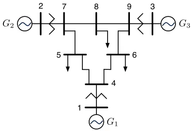
We illustrate the proposed methodology with the stan-dard three-machine-nine-bus Western Electricity Coordina-tion Council (WECC) power system, which is depicted in Fig. 1, it contains three synchronous generating units in buses 1,2 and 3, and load in buses 5, 6 and 8. The machine, network and load parameter values may be found in [18].
We consider one BA area for the WECC power system. As a result the ACE is only a function of the frequency deviation. We choose the frequency bias factor to beb= 0.1
MW/Hz. We formulate the ED process with the DCOPF, as
2 7 8 9 3
5 6
4
1
G1
[image:6.612.337.534.75.211.2]G2 G3
Figure 1: One-line diagram of the WECC three-machine nine-bus power system.
described in (4). The ED process is implemented every 5 minutes. The quantities in this section are expressed in per unit (p.u.) with respect to a 100 MVA base, unless stated otherwise. The load profile is as follows: PL5 +jQL5 =
1.25 +j0.50,PL6+jQL6 = 0.9 +j0.30, andPL8+jQL8=
1.00 +j0.35. The real power flow limits for all lines in the same (opposite) direction are 1 p.u. (−1p.u.). The cost functions for the three generators are (units are in $/MW):
ˆ
c1(PS1) = 0.025P
2
S1+ 10PS1+ 100,cˆ2(PS2) = 0.012P
2 S2+
20PS2+ 120andˆc3(PS3) = 0.010P
2
S3+ 13PS3+ 150. The
minimum (maximum) output in p.u. for each generator are:
0 ≤ PS1 ≤ 1.2, 0 ≤ PS2 ≤ 2 and 0 ≤ PS3 ≤ 1.5. The
ramping characteristics for each unit in MW/min are:κ+1 = 3,κ+2 = 2,κ+3 = 1andκ−1 =−3,κ−2 =−2andκ−3 =−1.
In initial steady state, there is no congestion in the system, thus the uniform LMP for the system is20.01 $/MW. The synchronous generators in buses 1 and 3 are at their upper limits. The dual variables associated with the upper limits for the two generators are ηM
1 = 9.95 $/MW and ηM3 = 6.98 $/MW. The timeframe of the simulations is described as follows: t = 0s a disturbance occurs, t = 60s the ED sends new signals to the generators and the AGC system is implemented every2s. In the first case, we modify the load in bus5 as followsPL5 = 1.7 p.u.. In this case, the results
0 20 40 60 80 100
58.5 59 59.5 60 60.5
f
[H
z]
t[s]
proposed method method A1 method A2
[image:6.612.326.546.584.698.2]0 10 20 30 40 50 60 0
2 4 6 8
c1
[$
]
t[s]
[image:7.612.334.553.73.191.2]proposed method method A1 method A2
Figure 3: Cost associated with AGC service for generator 1, with the three methods.
of the updated ED process, show that congestion arises in the system and the LMPs at each node are λ1 = 24.87,
λ2 = 20.02, λ3 = 13.03, λ5 = 29.02, λ6 = 15.17 and
λ8 = 22.85 in $/MW. We have 6 LMPs because in the
DCOPF formulation buses 1 ≡4,2 ≡7 and 3 ≡9, since they are connected by transformers.
The modification of the load causes a mismatch between generation and demand, and a deviation from the nominal frequency. We use three methods to allocate the AGC signal to restore the frequency to the nominal value: (i) our proposed method, (ii) alternative method A1 and (iii) alternative method A2. We compare the costs and the quality of AGC service for each method. For the WECC system we choose the value of ζ to be 2 $ min/MW2. The calculated values of the marginal cost in $/MW for each generator are ρ1 = 10.06, ρ2 = 20.02 and ρ3 = 13.03. We would
expect that the participation factor for generator1would be the largest; however, since we also consider the network constraints, we end up with ξ1 = 0.3710, ξ2 = 0.1653
andξ3= 0.4637 at first. The participation factors after the
updated ED process are: ξ1 = 0.3220, ξ2 = 0.3012 and
ξ3= 0.3768. Since, at first the LMPs are equal at all nodes,
in method A1, we have thatξi(A1) = 31, fori= 1,2,3. Then,
when the ED signal is updated and there is congestion in the system the participation factors becomeξ1(A1)= 0.2853,
0 20 40 60 80 100
−0.1 0 0.1 0.2 0.3 0.4
PS
1
−
PE D1
[p
.u
.]
t[s]
[image:7.612.76.286.78.191.2]proposed method method A1 method A2
Figure 4: Participation of generator 1 in the AGC system, with the three methods.
0 10 20 30 40 50 60
0 2 4 0 2 4 0
c2
[$
]
t[s]
[image:7.612.70.287.573.686.2]proposed method method A1 method A2
Figure 5: Cost associated with AGC service for generator 2, with the three methods.
ξ2(A1) = 0.3272 andξ3(A1) = 0.3876. For method A2, we
have constant participation factors for the considered period of time, which are equal to ξ1(A2) = 0.5, ξ2(A2) =
1 3 and
ξ3(A2) =
1 6.
The system’s frequency is depicted in Fig. 2. We notice that the AGC system serves its purpose, i.e., restores the frequency to its nominal value, with all three methods. The associated total cost for AGC service in $ for each method are: c= 55.3738,c(A1)= 55.3543andc(A2)= 56.7635for
the considered time period[0,100]sec. The minimum cost is achieved by using method A1, as was expected, however in this case the quality of service (ramping characteristics) is not taken into account. In method A2, the cost is high but the fastest unit is mostly used to meet the AGC demands. In Fig. 3, we depict the cost for AGC service offered from generator 1 for all three methods. We only plot the cost until
60s, because after the new signals are sent from the ED, the participation of the units as well as the associated costs are small. Generator 1 has the highest ramp rate in the system. Thus, as we can see form the graph the cost associated with A2 is the highest. The lowest cost is observed with A1, since the participation of generators based on A1 is uniform and does not consider the ramp rates. The proposed method provides a balance between the two as shown in Fig. 3. A modification of the parameter ζ gives more significance to
0 20 40 60 80 100 0
0.2 0.4 0.6 0.8 1
PC
2
[p
.u
.]
t[s]
proposed method method A1 method A2
Figure 6: The AGC signal for generator 2 PC2, with the
[image:7.612.327.549.575.686.2]0 200 400 600 800 1000 0
1 2 3 4
PC
[p
.u
.]
t[s]
PC1 PC
[image:8.612.76.288.75.193.2]2 PC3
Figure 7: The AGC signal for all generators, with ς = 0.1.
the cost or the quality of the AGC service. The participation of generator 1 in AGC is depicted in Fig. 4. We notice that after the new signal form the ED att= 60s, the AGC signals of all methods are similar and have small values.
In Fig. 5, we depict the cost of AGC associated with gen-erator 2. Both A1 and A2 assign a participation factor of 13, thus the costs associated with A1 and A2 are identical. The proposed method utilizes generator 2 in a lower extent, since the marginal costρ2 is the highest and the ramp rate of the
generator is2MW/min, which is in between the ramp rates of the other two generators. In Fig. 6, we depict the AGC signal to generator 2 PC2. Method A1 uniformly allocates
the AGC signal among the generators, until the ED signal is updated and the LMP at bus2becomes20.02$/MW, which is higher than the LMP at bus3, therefore the participation factor becomes ξ2(A1) = 0.3272<
1
3 and the participation
of generator 3 is greater, withξ3(A1) = 0.3876. The LMP at
bus 1 isλ1= 24.87 $/MW, which is greater than the LMP
at bus 2 λ2 = 20.02$/MW, thusξ1(A1) = 0.2853< ξ2(A1).
However, method A1 neglects the economic signalsηm i and
ηM
i associated with the lower and upper limit constraints for
each generator i. Even if the LMP at bus2 is smaller than that of bus1, the associated benefit of relieving the constraint associated with the upper limit of generator1isηM
1 = 14.81
$/MW. Thus, the marginal cost of generator1is10.06$/MW which is smaller than that of generator 2, which is 20.02
$/MW. That is why the participation factor of our proposed
0 200 400 600 800 1000
−1 0 1 2 3 4
PC
[p
.u
.]
t[s]
PC1 PC
[image:8.612.329.551.76.193.2]2 PC3
Figure 8: The AGC signal for all generators, with ς = 0.5.
0 200 400 600 800 1000
−1 0 1 2 3 4
PC
[p
.u
.]
t[s]
PC1 PC
[image:8.612.331.548.573.686.2]2 PC3
Figure 9: The AGC signal for all generators, withς = 0.8.
method for generator2 ξ2= 0.3012is smaller than that of
method A1: ξ2(A1) = 0.3272 and ξ1 = 0.3220 > ξ1(A1).
Generator 2 has κ+2 = 2, therefore method A2 assigns a
participation factor of 13 to generator2.
We present another case by modifying the system, in order to demonstrate the capabilities of the proposed method, where the generators’ cost functions are not overlapping and the system is not congested. We increase the line flow limits to3p.u. and the generators’ limits to5p.u.. We now select non intersecting cost functions (units are in $/MW):
ˆ
c1(PS1) = 0.010P
2
S1+ 10PS1+ 100,cˆ2(PS2) = 0.014P
2 S2+
15PS2 + 125 and ˆc3(PS3) = 0.025P
2
S3 + 20PS3 + 160.
The ramping characteristics for each unit in MW/min are:
κ+1 = 1, κ+2 = 2, κ+3 = 3 and κ−1 =−1, κ−2 = −2 and
κ−3 =−3. Since the generators limits are much higher than the total load, only the least cost unit is dispatched. In this case, we have PS1 = 3.3 p.u. and PS2 = PS3 = 0. The
system LMP is 10.06 $/MW. A modification in the load occurs at time t = 0s and we have PL5 = 1.7 p.u.. In
this case study we vary the parameter ζ to illustrate the modifications in the AGC signal among the generators. The parameters used for the determination of ζ are ρ¯= 15.02
$/MW and¯κ+= 2MW/min for this particular system. The
reasonρ¯is higher than the LMP is that generators 1 and 2 are at their lower limits. Then we modify the ratioς, i.e., we modify the variability of the net load. The values of ς, for
0 100 200 300 400 500 600
0 0.05 0.1 0.15 0.2 0.25
PS
2
−
PE D2
[p
.u
.]
t[s]
proposed method method A1 method A2
[image:8.612.69.287.585.701.2]0 100 200 300 400 500 600 0
2 4 6 8
c2
[$
]
t[s]
[image:9.612.76.288.78.191.2]proposed method method A1 method A2
Figure 11: Cost associated with AGC service for generator 2, with the three methods.
which the AGC allocations are depicted in Figs 7-9, are0.1,
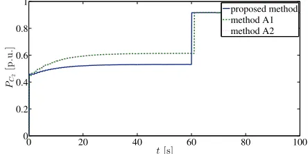
0.5 and0.8 respectively. We notice that as we increase the value of ς the more expensive but faster ramping units are used in regulation. For small values of ς only the cheapest generator, i.e., generator 1, participates in the AGC system, as seen in Fig. 7. Once, we increase the value ofς, we notice that the other two more expensive generators participate in the AGC system, as is depicted in Fig. 8. When, the value of
ςexceeds a certain value, that is0.8in this particular system, only the fastest generator is used in the AGC system, as it may be seen in Fig. 9. We notice in all figures that once the ED sends the new signal, at t= 60s, the entire load is met by generator 1 and the outputs of the other two generators are set to zero.
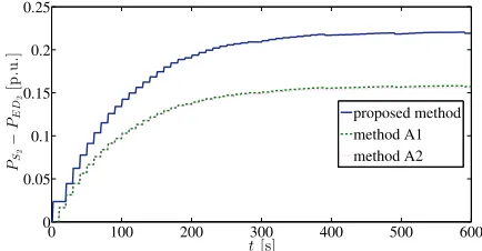
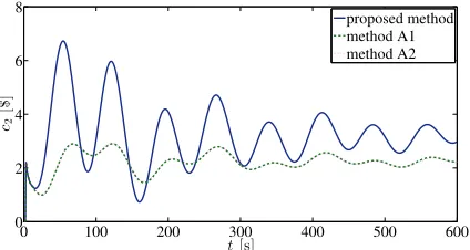
Now, we fix the value ofς to0.5and compare the results of the proposed method with the two alternative methods. As it may be seen from Fig. 10, the two alternative methods assign equal participation of generator 2 in the AGC system equal to 13. For ς = 0.5, the proposed method assigns a higher participation equal to 0.48, since the generator provides a good balance between the cost and the ramp rate. Generator 2 is more expensive than generator 1 but cheaper than generator 3. In addition, its ramp rate is 2
MW/min, which is in between the ramp rates of the other two generators. The cost associated with the AGC service offered by generator 2 is shown in Fig. 11. The cost is higher for the proposed method because the unit is utilized more with the proposed method than with the other two.
V. CONCLUDINGREMARKS
In this paper, we presented a systematic method of al-locating the AGC signal among the generators by taking into consideration the quality of the AGC service as well as economic criteria. In our modeling approach, we include the ED process, we represent the power system’s dynamics and incorporate network and other physical constraints. We use the information from the ED process to determine the marginal cost of increasing/decreasing a generator’s output. We take into account the quality of service, i.e., how fast the generators respond, by including in the objective function
a parameter that quantifies the importance of using fast responsive units in AGC regulation. In the numerical studies, we compared the cost as well as the quality of AGC service among three different allocation methods and illustrated that the proposed methodology provides a good balance between cost and quality of AGC service offered. Furthermore, we modified the value of parameterζmand see its effect on the
AGC allocation.
REFERENCES
[1] (2013, Accessed Apr.) Glossary of terms used in NERC reliability standards. [Online]. Available: http://www.nerc. com/files/Glossary of Terms.pdf
[2] A. Wood and B. Wollenberg,Power Generation, Operation,
and Control. New York, NY: Wiley, 1996.
[3] D. P. Kothari and J. S. Dhillon,Power System Optimization.
PHI Learning Private Limited, 2011.
[4] S. Stoft, Power System Economics: Designing Markets for
Electricity. New York, NY: Wiley-IEEE Press, 2002.
[5] J. Kumar, K. H. Ng, and G. Sheble, “AGC simulator for
price-based operation, part 1: A model,”IEEE Transactions
on Power Systems, vol. 12, no. 2, pp. 527–532, May 1997.
[6] M. Scherer, E. Iggland, A. Ritter, and G. Andersson, “Im-proved frequency bias factor sizing for non-interactive
con-trol,” in Presented at the Cigre session 44, Paris, France,
August 2012.
[7] D. H. Curtice and T. W. Reddoch, “An assessment of load frequency control impacts caused by small wind turbines,”
IEEE Transactions on Power Apparatus and Systems, vol. PAS-102, no. 1, pp. 162–170, 1983.
[8] J. L. Rodriguez-Amenedo, S. Arnalte, and J. C. Burgos, “Au-tomatic generation control of a wind farm with variable speed
wind turbines,” IEEE Transactions on Energy Conversion,
vol. 17, no. 2, pp. 279–284, 2002.
[9] Q. Liu and M. Ilic, “Enhanced automatic generation control
(e-agc) for future electric energy systems,” in IEEE Power
and Energy Society General Meeting, 2012, pp. 1–8.
[10] L. Wang and D. Chen, “Extended term dynamic simulation
for AGC with smart grids,” inIEEE Power and Energy Society
General Meeting, July 2011, pp. 1–7.
[11] D. Apostolopoulou, Y. C. Chen, J. Zhang, A. D. Dom´ınguez-Garc´ıa, and P. W. Sauer, “Effects of various uncertainty
sources on automatic generation control systems,” in IREP
Symposium-Bulk Power System Dynamics and Control -IX, August 2013.
[12] J. M. Arroyo and A. J. Conejo, “Optimal response of a power generator to energy, agc, and reserve pool-based markets,”
[13] I. Ibraheem, P. Kumar, and D. P. Kothari, “Recent philoso-phies of automatic generation control strategies in power
systems,” IEEE Transactions on Power Systems, vol. 20,
no. 1, pp. 346–357, 2005.
[14] H. Bevrani and T. Hiyamag,Intelligent Automatic Generation
Control. Taylor and Francis Group, LLC, 2011.
[15] (2013, Accessed Aug.) Frequency regulation compensation
in the oganized wholesale power markets. [Online].
Available: http://www.ferc.gov/whats-new/comm-meet/2011/ 102011/E-28.pdf
[16] Y. G. Rebours, D. S. Kirschen, M. Trotignon, and S. Rossig-nol, “A survey of frequency and voltage control ancillary
services – part ii: Economic features,”IEEE Transactions on
Power Systems, vol. 22, no. 1, pp. 358–366, 2007.
[17] (2013, Accessed Aug.) Market operations manual. [Online]. Available: http://www.iso-ne.com/rules proceds/isone mnls/ m 11 market operations revision 35 12 01 10.doc
[18] P. W. Sauer and M. A. Pai, Power System Dynamics and
Stability. Upper Saddle River, NJ: Prentice Hall, 1998.
[19] W. Y. Ng, “Generalized generation distribution factors for
power system security evaluations,” IEEE Transactions on
Power Apparatus and Systems, vol. PAS-100, no. 3, pp. 1001– 1005, 1981.
[20] A. S. Debs,Modern Power Systems Control and Operation.
Kluwer Academic Publishers, 1988.
[21] I. Griva, S. G. Nash, and A. Sofer,Linear and Nonliner
Op-timization. Society for Industrial and Applied Mathematics, 2009.
[22] Y. V. Makarov, C. Loutan, M. Jian, and P. de Mello, “Op-erational impacts of wind generation on california power
systems,” IEEE Transactions on Power Systems, vol. 24,
no. 2, pp. 1039–1050, 2009.
[23] (2013, Accessed Aug.) Analysis of ISONE balancing
requirements: Uncertainty-based secure ranges for iso
new england dynamic interchange adjustments.