Continuous and quad-graph integrable models with a boundary: Reflection maps and 3D-boundary consistency

City, University of London Institutional Repository

Citation: Zhang, Cheng (2013). Continuous and quad-graph integrable models with a

boundary: Reflection maps and 3D-boundary consistency. (Unpublished Doctoral thesis, City University London)

This is the unspecified version of the paper.

This version of the publication may differ from the final published

version.

Permanent repository link: http://openaccess.city.ac.uk/3016/

Link to published version:

Copyright and reuse: City Research Online aims to make research

outputs of City, University of London available to a wider audience.

Copyright and Moral Rights remain with the author(s) and/or copyright

holders. URLs from City Research Online may be freely distributed and

linked to.

City Research Online: http://openaccess.city.ac.uk/ [email protected]

Thesis

Continuous and Quad-Graph

Integrable Models with a Boundary:

Reflection Maps and

3

D

-Boundary Consistency

Cheng Zhang

Submitted in accordance with the requirements for the degree of

Doctor of Philosophy

Department of Mathematical Sciences

City University, London

iii

The life was limited,

the knowledg was unlimited. It wouldn’t be wise,

if thee trying to conquer the unlimited with the limited.

v

Acknowledgments

First of all, I would like to express my sincere gratitude to my supervisor Dr. Vincent

Caudrelier, for his advice, guidance and encouragement throughout the course of this

work. Special thanks to Dr. Nicolas Cramp´e for his valuable advice and discussion.

Many thanks to the staff in the Department of Mathematical Sciences at City

Uni-versity London, in particular to Prof. Andreas Fring, Dr. Olalla Castro Alvaredo,

Andrea Cavaglia and Emanuele Levi. Also, I would like to extend my appreciation to my internal examiner Prof. Joe Chuang and external examiner Prof. Alexander

P. Veselov for their extremely careful reading and remarkably precious comments.

vii

Abstract

This thesis is focusing onboundary problems for various classical integrable schemes. First, we consider the vector nonlinear Schr¨odinger (NLS) equation on the half-line. Using a B¨acklund transformation method which explores thefolding symmetry of the system, classes of integrable boundary conditions (BCs) are derived. These

BCs coincide with thelinearizable BCs obtained using the unified transform method

developed by Fokas. The notion of integrability is argued by constructing an explicit generating function for conserved quantities. Then, by adapting amirror image tech-nique, an inverse scattering method with an integrable boundary is constructed in

order to obtain N-soliton solutions on the half-line, i.e. N-soliton reflections. An interesting phenomenon of transmission between different components of vector

soli-tons before and after interacting with the boundary is demonstrated.

Next, in light of the fact that the soliton-soliton interactions give rise to

Yang-Baxter maps, we realize that the soliton-boundary interactions that are extracted

from theN-soliton reflections can be translated into maps satisfying the set-theoretical counterpart of the quantum reflection equation. Solutions of the set-theoretical re-flection equationare referred to asreflection maps. Both the Yang-Baxter maps and the reflection maps guarantee the factorization of the soliton and

soliton-boundary interactions for vector NLS solitons on the half-line.

Indeed, reflection maps represent a novel mathematical structure. Basic notions

such as parametric reflection maps, their graphic representations and transfer maps

are also introduced. As a natural extension, this object is studied in the context

of quadrirational Yang-Baxter maps, and a classification ofquadrirational reflection maps is obtained.

Finally, boundaries are added to discrete integrable systems on quad-graphs. Triangle configurations are used to discretize quad-graphs with boundaries.

Re-lations involving vertices of the triangles give rise to boundary equations that are used to described BCs. We introduce the notion of integrable BCs by giving a

three-dimensional boundary consistencyas a criterion for integrability. By exploring the correspondence between the quadrirational Yang-Baxter maps and the so-called

ABS classification, we also show that quadrirational reflection maps can be used as

a systematic tool to generate integrable boundary equations for the equations from

Contents

1 Introduction 1

1.1 2D soliton theories . . . 2

1.2 Yang-Baxter equation and reflection equation . . . 5

1.3 Yang-Baxter maps . . . 6

1.4 Discrete integrable systems . . . 7

1.5 Outline of thesis . . . 9

I

From the vector NLS equation on the half-line to

re-flection maps

10

2 ISM for the vector NLS equation 11 2.1 From Lax pair to RH problem . . . 11

2.2 Dressing transformations . . . 16

2.3 N-soliton solutions . . . 20

3 The vector NLS equation on the half-line 25 3.1 Deriving integrable boundary conditions . . . 26

3.2 Check of integrability . . . 31

3.3 Mirror image construction . . . 33

3.4 Example of one-soliton reflections . . . 37

4 Factorization of soliton-soliton and soliton-boundary interactions 41 4.1 Factorization ofN-soliton interactions . . . 42

4.2 Factorization ofN-soliton reflections . . . 47

5.2 N-soliton reflections . . . 59

II

Reflection maps: classification and applications

62

6 Set-theoretical reflection equation and reflection maps 63 6.1 Yang-Baxter maps . . . 63

6.2 Reflection maps . . . 66

7 Reflection maps for quadrirational Yang-Baxter maps 71 7.1 Quadrirational Yang-Baxter maps . . . 71

7.2 Deriving reflection maps . . . 75

7.3 Classification of reflection maps . . . 79

8 Quad-graph integrable systems with boundary 82 8.1 3D-consistent equations on quad-graphs . . . 83

8.2 Boundary conditions for quad-graph systems . . . 86

8.3 Integrability: the 3D-boundary consistency . . . 88

8.4 From reflection maps to boundary equations . . . 91

8.5 Boundary equations for A1_δ=0 as an example . . . 95

9 Conclusion 99 Appendices 101 A Unified transform method and linearizable boundary conditions 102 A.1 From Lax pair to global relation . . . 103

A.2 Linearizable boundary conditions . . . 107

B Proof of Eq. (3.25) 109

C Algorithm for constructing paired norming constants 113

D Proof of Prop. 4.2.1 115

E Reflection maps for H_II 118

F Quad-graph equation-Yang-Baxter map correspondence 119

G Boundary equations for the ABS classification 122

Chapter

1

Introduction

Since the birth of the modern theories of integrability dated back to the late 1960s,

integrable systemshave been extensively studied as one of the most attractive fields in mathematical physics. Probably, the most striking feature of integrable systems is that certain nonlinear systems can be exactly solved by mathematical methods and such systems exhibitsoliton solutionsthat are particle-like objects interacting elasti-cally with themselves. Nowadays, these nonlinear systems are qualified as integrable

and believed to be widely involved in our understanding of natural phenomena. The

appearance of integrable systems has been marked in almost every single branch

of physics, and the impact has reached far to areas ranging from fiber optics, that

engineers the transmissions of information and ensures our everyday

communica-tions, through the experiments in atomic physics, aiming to understand the utter

properties of atoms and molecules, to the attempts of speculating some of the most fundamental problems in physics using concepts developed around string theory and

conformal field theory. Numerous mathematical methods have also been developed

and found to have deep connections to different areas of pure mathematics. So far,

integrable systems have become a powerful tool to understand physics and develop

new concepts and methods in mathematical physics.

Amongst the very rich topics in integrable systems, boundary problems arise as one of the fundamental problems in the discipline. Indeed, most of models are

known to be integrable only in the presence of very special boundary conditions

such as periodic boundary conditions. Adding more generic boundary conditions to integrable systems signifies a better description of physics, since real physical systems

naturally involving boundaries. From the point of view of integrability, deriving

integrable boundary conditions—boundary conditions that preserve the integrability property—consists of a highly non-trivial task.

integrable models. We start, in this chapter, by giving a general introduction to the

areas of study that are relevant to the thesis.

1.1

2

D

soliton theories

Two-dimensional (2D) soliton models, namely models possessing soliton solutions, are 2D—one dimensional space plus time—nonlinear partial differential equations that can be exactly solved by means of the inverse scattering method.

Historically, the development of soliton theories also marked the birth of the

integrable theories. The story can be traced back to the late 19th century when the mathematicians in that epoch derived the Korteweg-de Vries (KdV) equation [30, 80] in the context of fluid dynamics. This equation is in the following simple

form for a real field u(x,t):

u_t+u_xxx+6u u_x=0, (1.1) where the subscripts mean the partial derivatives1. After more than a half-century of its introduction, the KdV equation was revived in 1965 by Zabusky and Kruskal [120]. Using a numeric method, they discovered that Eq. (1.1) exhibits particle-like

solutions that interact elastically with themselves. Apparently counter-intuitive, this

particular type of solutions was named as solitons and gave an adequate explanation

to the Fermi-Pasta-Ulam problem [49], a puzzle initiated in numeric experiments. Mathematical foundations for solitons were soon established notably following the

inventions of the inverse scattering method [61] and theLax pair [81] which created an elegant framework to solve the KdV equation. Gradually, soliton solutions were

found in many other models such as the nonlinear Schr¨odinger equation [123], the modified KdV equation [116] and the sine-Gordon equation [7]. The notions of integrability such as infinite conservation laws [90, 81], Hamiltonian structure [60,

122] and B¨acklund transformations [117] were also clarified. Solitons have thus become a characteristic feature of integrable systems.

One-soliton solution of the KdV equation is the following traveling wave function:

u(x,t) = 1

2csech

2

√

c

2 (x−ct−a)

, c,a∈_R, (1.2) wherecis a real parameter controlling both the velocity and the amplitude ofu(x,t). This wave maintains its shape while it travels at constant speed. To understand

soli-ton phenomena, let us look back at the form of (1.1). There are two sources of force

1.1. 2DSOLITON THEORIES 3

coexisting: on one hand, the dispersion, coming from the linear term ut+uxxx that physically tries to extend the wave envelope, and on the other, thedissipation, com-ing from the nonlinear term 6u u_x that basically tries to destroy the wave envelope. Then, the fact that (1.1) exhibits solutions like (1.2) can be understood as a ”magic”

balance between both the dispersion and the dissipation. In other word, to have

wave functions such as (1.2), the nonlinearity is an essential ingredient! Indeed,

observation of such waves had already been reported as ”solitary waves” [102] in the mid-19th century by the Scottish engineer Russell when he studied the motion of water. Next, one can ask the following questions: first, do any other physical

system governed by the KdV equation exist in nature? Second, does the ”magic”

balance between dispersion and dissipation exist for any other nonlinear system?

The answers for both questions are yes. Nowadays, we know that the KdV equation

appears in the context of acoustic waves traveling in crystals. Also, a wide range

of soliton models exist. It is argued that soliton models are, in fact, of universal

character and can be widely applied in describing Nature (see for instance [121]). A

powerful method for solving soliton models, known as the inverse scattering method (ISM) (the ISM will be explained in depth in Chapter 2), exists.

Another universal integrable model is the nonlinear Schr¨odinger (NLS) equation:

i u_t+u_xx−2λ|u|2u=0, λ=±1, (1.3)

where u is a complex-valued field depending on x and t. In the case λ=−1, that

is called focusing case for the nonlinear term −2λ|u|2u with λ=−1 arises as an

attractive ”force”, the NLS equation (1.3) possesses soliton solutions. Its one-soliton

solution can be written in the form

u(x,t) =a e−i(bx+(b2−a2)t+φ0)_{sech(a(x+2bt−∆c)), (1.4)}

wherea,bare parameters controlling the velocity and amplitude ofu(x,t)andφ0,∆c

are parameters characterizing respectively the initial phase and space position. As a single integrable model, the NLS equation has a great impact in both mathematics

and physics. In [123], Zakharov and Shabat first gave soliton solutions to the NLS

equation by generalizing the Lax pair [81]. This just built up the basis for the

later development in [7] in which a powerful framework of the ISM to generate and

solve soliton models, known as the AKNS scheme, was derived. Also, Manakov

generalized the NLS equation to a two-component coupled version [87], known as

Manakov system or vector NLS model, aiming at simulating electro-magnetic field

becoming the governing equation in the filed of fiber optics—solitons were reportedly

observed in experiments [68]—that is of great interest in engineering. The quantum

version of the NLS equation, known as Lieb-Liniger model that is used to describe a

gas of particles moving in one dimension and satisfying Bose-Einstein statistics, was

solved in [84]. This result inspired Yang who gave his famous rational solution of the

Yang-Baxter equation [119] by extending the spinless particles in [84] to particles

with spin. Note that both Manakov and Yang’s ideas lie in adding internal degrees of freedom to a scalar quantity. In the context of soliton theories, this gives rise to the

multi-component soliton models. The ISM for solving classes of multi-component

soliton models was extensively studied, for instance in [110].

Initial-boundary value problems, initiated in the study of partial differential

equa-tions, appear naturally in soliton theories. Since an early attempt [4] in which the

KdV equation on the half-line was considered, half-line problems for soliton models

have attracted much attention from many researchers. An idea of using B¨acklund transformation to construct integrable boundary conditions was first proposed by

Sklyanin in [103]. Later, in [25, 26, 66, 109], the B¨acklund transformation method was applied to the NLS and sine-Gordon equations for deriving integrable

bound-ary conditions. In [50], the NLS model was again treated by using analysis of the

linearized NLS equation. The common result of these two approaches consists in

representing the half-line system by folding a full line system. The vector NLS

equa-tion on the half-line was studied in [67] using an algebraic approach. Recently, a

nice mirror image construction was developed in [27] for the NLS equation, which

led toN-soliton solutions on the half-line.

On the other hand, Fokas has recently developed a powerful method [51, 52,

54], referred to as Fokas method or unified transform method (this method will be discussed in more detail in Appendix A), for treating boundary value problems for soliton equations. Roughly speaking, this method is based on a simultaneous analysis

of both parts of the Lax pair, which translates the initial-boundary conditions into

spectral functions in Fourier space. Then the solutions of the original system can be

obtained using certain inverse transforms from the spectral functions. The unified

transform method can be applied to a large class of boundary problems for soliton

equations ranging from half-line problems [52, 32, 57] and to systems defined on an

1.2. YANG-BAXTER EQUATION AND REFLECTION EQUATION 5

1.2

Yang-Baxter equation and reflection equation

The (quantum) Yang-Baxter equation, introduced separately by Yang [119] in the

context of quantum field theory and by Baxter [17] in the context of statistical

me-chanics, is at the heart of understanding quantum integrable models. The equation

can be written in the following form:

R

12

R

13

R

23=

R

23

R

13

R

12, (1.5)

where

_R

, commonly known as

_R

-matrix, is a matrix acting onV⊗V—V is a vector space—with the understanding that

_R

₁₂ =

_R

⊗_I,

_R

₂₃ =_I⊗

_R

and so on. From a

=

Fig. 1.1 : Yang-Baxter equation

physical point of view, as pointed out in [126], the Yang-Baxter equation describes

the factorization of anN-particle scattering, which is a unique feature displayed by

2Dintegrable systems (see Fig. 1.1). On the other hand from a mathematical point of view, the algebraic structures underlying the Yang-Baxter equation can be seen as

deformations of the usual Lie algebras or their infinite dimensional extensions: the

Kac-Moody algebras [77]. Such deformed algebraic structures are known nowadays

as quantum groups or quantum algebras [75, 76, 43].

In the context of quantum integrable systems with boundaries, there exists, in addition to the Yang-Baxter equation, a second equation: the reflection equation,

also known as the boundary Yang-Baxter equation [42, 104], that is used to encode

the interactions of quantum particles with boundaries. The equation is in the form

R

12

K

1

R

21

K

2=

K

2

R

12

K

1

R

21, (1.6)

where

_K

, also known as

_K

-matrix, is a matrix acting on V. The appearance of

K

in the reflection equation (1.6) can be seen as a certain consistency with the

R

-matrix. Then,

_K

, that describes the particle-boundary scattering, along with

as the factorization of both the particle-particle and particle-boundary scatterings.

2 1

2 1

=

Fig. 1.2 : Reflection equation

1.3

Yang-Baxter maps

One aspect of the Yang-Baxter equation (1.5) is that the

_R

-matrix is an operator

acting on tensor product of vector spaces,i.e.V⊗V, which allows the equation itself to have rich algebraic structures. However, one can ”relax” this property by replacing

V⊗V by S×S, where S is an arbitrary set and × means Cartesian product. This gives rise to the set-theoretical version of the Yang-Baxter equation, first suggested as a subject of study by Drinfeld in [44] (a solution was already obtained earlier by

Sklyanin [105]). Nowadays, solutions of the set-theoretical Yang-Baxter equation are

commonly accepted as Yang-Baxter maps, originating from a suggestion of Veselov [113]. The name rational set-theoretical

_R

-matrices also exists in the literature. With the understanding that

_R

is a map acting on S×S, the theoretical Yang-Baxter equation, which shares the same structure as the usual quantum Yang-Yang-Baxter

equation (1.5), is now read as a compatibility condition of two different ways to do

decompositions of maps.

Different aspects of Yang-Baxter maps have been developed and numerous

con-nections have been established with, for example, Poisson-Lie groups and

alge-bras [118, 70, 46, 86, 101], discrete Lax representation [106] and transfer maps

[113]. Yang-Baxter maps also arise in different contexts in mathematical physics,

such as geometric crystals [45], cellular automaton [107, 69, 58], factorization of multi-component solitons’ scattering [111, 64, 9] and discrete integrable systems

[98, 72, 79]. Note that, although the multi-component soliton theory is a

well-established discipline, it has only been understood, rather recently in [111, 9] for

1.4. DISCRETE INTEGRABLE SYSTEMS 7

scattering (or collision) factorizes into N

2

!

pairwise soliton scatterings, that can

be expressed in terms of Yang-Baxter maps. In [14], effort was put into

classify-ing Yang-Baxter maps in the case S=_CP1, which led to the important concept of

quadrirational maps. Classifications of quadrirational Yang-Baxter maps were also exhausted in [14, 97].

1.4

Discrete integrable systems

Recently, there has been an increasing interest in two-dimensional discrete integrable

systems. Practically, an important motivation comes from the use of computer

and numeric analysis which is naturally involved with discrete variables—soliton

solutions [120] of the KdV equations were first found by using numeric method!

Moveover, all the concepts and methods developed in the continuous theories can be found to have their deep roots in discrete systems. Nowadays, it is believed

that, in many aspects, discrete systems are more fundamental than their continuous

counterpart (see for instance [92]).

Early developments of the discipline lie in discretizing one variable (usually the

time variable) of certain known soliton systems [2, 3, 73, 74]. This corresponds

to semi-discrete systems or differential-difference systems. Discrete equations that

we are considering in this thesis are fully discrete systems or difference-difference

systems, which discretize both the space and time variables. Mainly following [94, 99]

by using the direct linearization method, a number of interesting discrete models were derived (see also [92]).

On the other hand, it is often possible to pass from a continuous equation to a

discrete equation via B¨acklund transformations. B¨acklund transformations in soliton theories are transformations which map solutions of a soliton equation into new

so-w

BT_λ

BTµ

b

w

BTµ

e

w

BT_λ e

b

w=e b

[image:18.596.222.406.604.725.2]

w

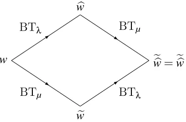
lutions. They are known to satisfy the Bianchi permutability property (see Fig. 1.3).

The most famous example is the discrete potential KdV (dpKdV) equation that can

be obtained using B¨acklund transformations for the KdV equation [117]. The con-struction is illustrated in Fig. 1.3. The field w is defined as w_x=u for u satisfying the KdV equation. Thanks to the permutability property, e

b

w and b e

w are compatible. Relation involvingw, w_e,w_band e

b

w is in the form

(w−e

b

w)(w_b−w_e) +4(λ−µ) =0, (1.7)

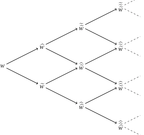
which is the dpKdV equation. In this way, discrete systems can be generated in a

lattice following successive applications of B¨acklund transformation (see Fig. 1.4).

[image:19.596.193.442.307.540.2]

w b w e w e e e w b e e w b b e w b b b w e e w b e w b b w

Fig. 1.4 : Lattice generated by B¨acklund transformations

There exist several notions and tests for integrability of discrete systems. Let

us mention for instance integrable mappings [112], algebraic entropy [23], singular-ity confinement [65] and three-dimensional consistency [91, 29]. The latter will be discussed in Chapter 8. In [29, 13], discrete integrable systems were extended to

quad-graphs,i.e.planar graph of cellular decompositions with quadrilateral faces (in contrast to the square lattice), and a classification of discrete integrable equations was accordingly given [13]. These laid the foundation for important developments

in discrete integrable systems. Some important results have already been achieved,

such as soliton generations [12, 93], Lagrangian structures [85] and discrete ISM [34],

1.5. OUTLINE OF THESIS 9

1.5

Outline of thesis

Following the two different types of the underlying integrable systems that we are

considering in this thesis, namely continuous and discrete, this thesis is naturally

divided into two parts. Motivations and notably notions of integrability will be

clarified in each precise context of this presentation.

In Part I—Chapter 2 - Chapter 5—we study the vector NLS equation on the

half-line. Chapter 2 reviews the ISM that is the basic instrument used throughout Part I.

In Chapter 3, classes of integrable BCs are derived. Soliton solutions on the half-line

are also constructed using a mirror image method. In Chapter 4, we introduce reflec-tion maps that satisfy the set-theoretical counterpart of the reflection equation, in order to prove the factorization of soliton-soliton and soliton-boundary interactions.

Another approach, called space-evolution method, to solve the vector NLS equation

on the half-line, is proposed in Chapter 5. Part II—Chapter 6 - Chapter 8—deals

with reflection maps and quad-graph systems with boundary. We study in detail the set-theoretical reflection equation and reflection maps in Chapter 6. Reflection

maps in the context of quadrirational Yang-Baxter maps are considered in

Chap-ter 7. In ChapChap-ter 8, boundaries are added to quad-graph systems. In particular, we

propose athree-dimensional boundary consistency as a criterion for integrability for quad-graph integrable systems with boundary. Concluding remarks are reported in

Chapter

2

ISM for the vector NLS equation

In this chapter, we review the inverse scattering method (ISM) for the vector NLS

equation, in order to collect results and notations needed in Part I of this thesis. The

main technical complexity of the vector generalization of the NLS model lies in the computation of the N-soliton scattering data that are encoded in a matrix quantity a+(k), in contrast to the scalar NLS case where a+(k) is a scalar. To overcome this difficulty, we use the approach based on theRiemann-Hilbert(RH) formulation. This leads to a powerful framework, by virtue of thedressing transformations, to compute a+(k) and the N-soliton solutions in a compact form. In particular, we put our emphasis on Theorem 2.2.7 which indeed reflects theBianchi permutativity property

in the context of dressing transformations. This theorem will play an important

role when we study the factorization of an N-soliton interaction in the forthcoming chapters. We refer readers to [5, 47, 6, 8] for more detailed presentations of the ISM, and to [124, 125, 47, 16, 62] for the dressing transformations.

2.1

From Lax pair to RH problem

The traditional approach of the ISM consists of three steps: 1) direct scattering

which transforms the soliton equation into a set of scattering data by using the x -part of the Lax pair; 2) time-evolution which makes the scattering data evolved in time by using the t-part of the Lax pair; 3) inverse scattering which reconstructs the solutions of the original soliton equation from the time-evolved scattering data.

With the help of the RH formulation, these three steps can naturally be absorbed

into the RH problem itself.

complex-valued vector field

R(x,t) =



  

r1(x,t)

.. .

r_n(x,t)



  

, (2.1)

we require that the jth component r_j(x,t), j=1, . . . ,n is a smooth enough function that vanishes to zero as x→ ±∞ for all t. This requirement corresponds to the

so-called vanishing boundary conditions1. The vector NLS equation is defined as

iR_t(x,t) +R_xx(x,t)−2λ(R†R)R(x,t) =0, (2.2)

where R†(x,t) is the transpose conjugate of R(x,t) and λ is the (real) coupling

con-stant which can be normalized to λ=±1. Define Q(x,t) as the following (n+1)×

(n+1)matrix-valued field:

Q(x,t) = 0 R(x,t)

λR†(x,t) 0

!

, (2.3)

the vector NLS equation (2.2) can be written as the compatibility condition (Φxt =

Φtx) of the two following linear problems, known as auxiliary problems orLax pair, for an (n+1)×(n+1) matrix-valued function Φ(x,t,k)2:

Φx+ik[Σ3,Φ] =QΦ, (2.4)

Φt+2ik2[Σ3,Φ] =QTΦ, (2.5) where

Σ3=

I_n 0 0 −1

!

, Q_T =2kQ−iQ_xΣ3−iQ2Σ3, (2.6)

with In being the n×n identity matrix. Eq. (2.4) and (2.5) represent respectively the x-part and t-part of the Lax pair.

Remark 2.1.1 The Lax pair for the vector NLS equation is also widely seen in the literature as two operators U and V satisfying the zero curvature condition:

U− ∂

∂x

,V− ∂

∂t

=0, (2.7)

1_{This requirement restricts the classes of solutions that we consider in this thesis, and detailed}

treatments can be seen for instance in [5, 47].

2.1. FROM LAX PAIR TO RH PROBLEM 13

whereU, V are defined as

U=−ikΣ3+Q(x,t), V =−2ik2Σ3+QT(x,t,k). (2.8)

The corresponding auxiliary problems turn out to be

Uψ=ψx, Vψ=ψt. (2.9)

For practical purposes, we work with the auxiliary problems (2.4, 2.5) that are simply related to (2.9) by specifying

ψ(x,t,k) =Φ(x,t,k)e−i(kx+2k

2_t)Σ

3_{. (2.10)}

From Eq. (2.3), one can observe that Qsatisfies

W QW−1=−Q†, (2.11) where

W = −λIn 0

0 1

!

. (2.12)

This implies that, provided thatΦ(x,t,k)is a solution of (2.4, 2.5),WΦ†(x,t,k∗)W−1

satisfies the same equations as Ψ(x,t,k)≡Φ−1(x,t,k) does,i.e.

Ψx+ik[Σ3,Ψ] =−ΨQ, (2.13)

Ψt+2ik2[Σ3,Ψ] =−ΨQT. (2.14) Following the vanishing boundary conditions, we are able to define two Jost solutions

X(x,t,k) andY(x,t,k)of (2.4, 2.5) satisfying

lim

x→−∞

eiφ(x,t,k)Σ3_X(x,t,k)e−iφ(x,t,k)Σ3_=I

n+1, k∈R, (2.15)

lim

x→∞

eiφ(x,t,k)Σ3_Y(x,t,k)e−iφ(x,t,k)Σ3_=I

n+1, k∈R, (2.16)

where

• Volterra integral representations:

X(x,t,k) =I_n+1+

Z x

−∞

e−ik(x−y)Σ3_{Q(y,t)X(y,t,k)e}ik(x−y)Σ3_{dy, (2.18)}

Y(x,t,k) =I_n+1+

Z x

∞

e−ik(x−y)Σ3_{Q(y,t)Y(y,t,k)e}ik(x−y)Σ3_{dy. (2.19)}

• Due to the traceless property of Q(x,t),

detX(x,t,k) =detY(x,t,k) =1. (2.20) • Since bothWΦ†(x,t,k∗)W−1 and Φ−1(x,t,k) satisfy (2.13, 2.14), one gets

W X−1(x,t,k)W−1=X†(x,t,k∗), W Y−1(x,t,k)W−1=Y†(x,t,k∗). (2.21) • X andY can be split into the following ”column” vectors3 forms:

X = (X+,X−), Y = (Y−,Y+), (2.22) where X+, Y+ (resp. X−, Y−) are analytic and bounded in the upper (resp. lower) half k-complex plane.

A straightforward calculation shows that ifΨ1andΨ2are two solutions of (2.4, 2.5),

then they satisfy

Ψ1(x,t,k) =Ψ2(x,t,k)e−iφ(x,t,k)Σ3T(k)eiφ(x,t,k)Σ3, (2.23)

where the (n+1)×(n+1) matrix T depends on the spectral parameter k only. Therefore, we define the matrix S(k) that relates the Jost solutionsX andY as

X(x,t,k) =Y(x,t,k)e−iφ(x,t,k)Σ3_S(k)eiφ(x,t,k)Σ3_{, k∈}

R. (2.24)

It follows from the properties ofX andY thatdetS(k) =1, and S(k)can be split into block matrices of natural sizes4:

S(k) = a

+_{(k) b}−_(k)

b+(k) a−(k)

!

. (2.25)

3_{Here, the left ”column” vector is made of the first left n columns and the right one is made}

of the remaining column. This column vector representation will be constantly used in the rest of this thesis.

2.1. FROM LAX PAIR TO RH PROBLEM 15

Again, a±(k) are understood to be analytic in _C±, where _C+ and _C− are used to denote the upper and lower half k-complex planes respectively. Moreover, one has

W S(k)−1W−1=S†(k∗). (2.26) LetS(k)−1 be written in components as

S(k)−1= c

−_{(k) d}−_(k)

d+(k) c+(k)

!

, (2.27)

where c∓(k) allow for analytic continuations into _C∓. The relation (2.26) can be explicitly translated into

(a±)†(k∗) =c∓(k), b±(k∗) =−λ(d∓)†(k), (2.28)

with the functions defined in the appropriate domains.

Remark 2.1.2 For the scattering system (2.24), there are two equivalent sets: {a±,b±}

and {c±,d±}, known as the minimal set of scattering data [62], which are available to reconstruct R(x,t) in the inverse part of the ISM. Without loss of generality, we choose to work with {a±,b±} in the rest of this thesis.

A crucial observation in the development of the ISM, originated from the work

of Manakov [87] and Zakharov and Shabat [124], is that the scattering system (2.24)

can be formulated as an RH problem and this RH problem is equivalent to the ISM

associated with the Lax pair (2.4, 2.5). We state the following propositions which

are well-known in the soliton theory. Proofs can be found, e.g., in [47, 54].

Proposition 2.1.3 The scattering system defined in (2.24) can be rewritten as the following RH problem

J+(x,t,k)J−(x,t,k) =e−iφ(x,t,k)Σ3_J(k)eiφ(x,t,k)Σ3_{, k∈}

R, (2.29)

and

lim

|k|→∞

J±(x,t,k)→I_n+1. (2.30)

Here J±(x,t,k) are analytic and bounded matrix-valued functions in _C±, defined as

J+(x,t,k) = a

+_{(k) 0}

0 c+(k)

!

(X+,Y+)−1(x,t,k), J−(x,t,k) = (Y−,X−)(x,t,k),

and J(k) is the jump matrix defined as

J(k) = In b

−_(k)

d+(k) 1

!

, k∈_R. (2.32)

In particular, we have

detJ+(x,t,k) =deta+(k), detJ−(x,t,k) =a−(k). (2.33) Proposition 2.1.4 Assume that the above RH problem (2.29, 2.30) has unique so-lutions J±(x,t,k) which are sufficiently smooth for all (x,t)∈_R. Then J+(x,t,k)

(resp. J−(x,t,k) ) satisfies the Lax pair (2.13, 2.14) (resp. (2.4, 2.5)). In particu-lar, J+(x,t,k) gives a uniquely defined Q(x,t) in the form

Q(x,t) = lim

|k|→∞

−ik[Σ3,J+(x,t,k)]. (2.34)

Eq. (2.34) is called reconstruction formula.

Thanks to Prop. 2.1.3 and 2.1.4, the original problem of solving the vector NLS

equation is now translated into the matrix RH problem (2.29, 2.30). Therefore, the

ISM mainly consists of the following two steps: 1) to formulate an RH problem via the scattering system (2.24); 2) to solve the RH problem that will lead to the solu-tions of (2.2) via the reconstruction formula (2.34). Although in general one cannot solve a matrix RH problem explicitly, a powerful method exists inside such

formal-ism for constructing its singular solutions which will correspond to soliton solutions.

This method is precisely the dressing transformations that will be introduced in the

following section.

2.2

Dressing transformations

In the context of soliton theory, dressing transformations were first introduced by

Zakharov and Shabat in [124, 125]. Here, we present the dressing transformations

and their connections to an RH problem in a general context. The application

to the vector NLS case, which consists of a special reduction, will be treated in

the next section. The main result lies in Theorem 2.2.7 which in fact reflects the Bianchi permutativity property. A system of notations, that captures this property

is accordingly introduced. We refer readers to [16] for details and in particular for

the proofs of Prop. 2.2.3 and 2.2.4. The study of matrix RH problems in a more

2.2. DRESSING TRANSFORMATIONS 17

Consider the following matrix RH problem with canonical normalizations:

J

+_(k)

_J

−_{(k) =}

_J

_{(k), k∈}

R, lim

|k|→∞

J

±_{(k)→I, (2.35)}

where

_J

(k) is the jump matrix satisfying det

_J

(k)=6 0 for k∈_R. The matrix

_J

+(k)

(resp.

_J

−(k)) is analytic in _C+ (resp. _C−). This problem has unique regular solutions

_J

₀±(k), and the term ”regular” means that det

_J

₀±(k)6=0 in the appropriate domain. By contrast, we specify the term ”singular” in our context by the following

definitions.

Definition 2.2.1 A matrix functionM(k)is said to be singular atk=k₀ifdetM(k₀) =

0 and if in the neighborhood of k₀

M(k) =M₀+ (k−k₀)M₁+O(k−k₀)2, M−1(k) = N0

k−k0

+N₁+O(k−k₀). (2.36) Definition 2.2.2 An RH problem with zeros or poles at k±_j ∈_C±, j=1, . . . ,N is an RH problem as defined in (2.35) where

_J

±(k) are singular at k±_j, j=1, . . . ,N.

Given these two definitions, one can prove the following.

Proposition 2.2.3 Fixing the subspaces

_V

j≡Im

J

+(k)|_k=k+

j and

U

j≡Ker

J

−_(k)|

k=k−_j,

j =1, . . . ,N determines uniquely the solution of the RH problem with zeroes at

k±_j ∈_C±.

In general, there is no known closed-form formula to solve a matrix RH problem.

However, once the regular solutions are known, it is possible to construct singular

solutions from them.

Proposition 2.2.4 Let

_J

±(k) be the singular solutions at k±₀ ∈_C± with

Im

_J

+(k)

k=k+₀ =

V

0, Ker

J

−_(k)

k=k−₀ =

U

0, (2.37)

and let

_J

₀±(k) be the solution of the same RH problem regular at k₀±. Then

_J

±(k)

can be written as

J

+_{(k) =}

_J

+

0 (k)

I+k

−

0 −k

+

0

k−k−₀ Π0

,

_J

−(k) =

I+k

+

0 −k

−

0

k−k₀+ Π0

J

0−(k). (2.38)

Here Π0 is a projector defined as

KerΠ0=

J

₀+(k+₀)

−1

The form of singular solutions (2.38) introduces what are called dressing factors

(of degree 1) which transform

_J

₀±(k) regular at k₀± into

_J

±(k) singular at k₀±. This gives an algorithm to construct singular solutions

_J

±(k) at distinct k±_j ∈_C±, j=

1, . . . ,N from regular solutions

_J

₀±(k). Precisely, let k±_j ∈_C±, j=1, . . . ,N and the corresponding subspaces

_V

j,

U

j be given, we can use Prop. 2.2.4 repeatedly to

construct

_J

±(k) singular at k±_j recursively from

_J

₀±(k) starting from k±₁, k±₂ up to

k±_N. Consequently,

_J

±(k) can be written as

J

+(k) =

_J

₀+(k)

I+k

−

1 −k

+

1

k−k−₁ Π1

. . .

I+k

−

N−k + N

k−k_N− ΠN

, (2.40)

J

−(k) =

I+k

+ N−k

−

N

k−k_N+ ΠN

. . .

I+k

+

1 −k

−

1

k−k+₁ Π1

J

0−(k), (2.41)

where, for j=1, . . . ,N

KerΠj=

J

₀+(k+_j ) I+

k₁−−k+₁ k+_j −k−₁ Πj−1

!

. . . I+k

−

j−1−k

+ j−1

k+_j −k−_j−1 Π1

!!−1

V

j, (2.42)

ImΠj= I+

k+_j−1−k−_j−1 k−_j −k+_j−1 Πj−1

!

. . . I+k

+

1 −k

−

1

k−_j −k₁+Π1

!

J

0−(k

−

j )

U

j. (2.43) Now comes a fundamental observation: in the above construction, one can iterate the

construction of

_J

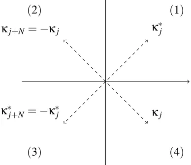
±(k)by using a different order on thek±_j . Let

_S

Nbe the permutation group on the set {1, . . . ,N} and let σ∈

S

N. Denote the image of (1, . . . ,N) under σ

by(σ(1), . . . ,σ(N)) and introduceκ±_j =k±_σ(j). Then, the subspaces corresponding to κ±_j are

V

_σ(j),

U

_σ(j). Repeating the previous procedure, starting from κ±₁ up to κ±_N,

one gets

˜

J

+_{(k) =}

_J

+

0 (k)

I+κ

−

1 −κ

+

1

k−κ−₁ Πσ₁

. . .

I+κ

−

N−κ + N

k−κ−_N Πσ_N

, (2.44)

˜

J

−(k) =

I+κ

+ N−κ

−

N

k−κ+_N Π

σ N

. . .

I+κ

+

1 −κ

−

1

k−κ+₁ Π

σ

1

J

0−(k), (2.45)

where, for j=1, . . . ,N,

KerΠσ_j =

J

₀+(κ+_j) I+κ

−

1 −κ

+

1

κ+_j −κ−₁ Π

σ j−1

!

. . . I+κ

−

j−1−κ

+ j−1

κ+_j −κ−_j−1 Π

σ

1

!!−1

V

σ(j), (2.46)

ImΠσ_j = I+

κ+_j−1−κ−_j−1 κ−_j −κ+_j−1

Πσ_j−1

!

. . . I+κ

+

1 −κ

−

1

κ−_j −κ+₁ Πσ₁

!

J

0−(κ

−

2.2. DRESSING TRANSFORMATIONS 19

V

j= Im ˜

J

+(k)

k=k+_j ,

U

j= Ker ˜

J

−_(k)

k=k−_j , (2.48)

j=1, . . . ,N, so that Prop. 2.2.3 implies that

_J

˜±(k) =

_J

±(k). In turn, this implies that the product of dressing factors in (2.44, 2.45) is equal to the product of dressing

factors in (2.40, 2.41). This construction introduces the notion of dressing factors of

degreeN which transform

_J

₀±(k) into

_J

±(k)singular at k±_j, j=1, . . . ,N. Prop. 2.2.3 also ensures that a dressing factor of degree N factorizes into N dressing factors of degree 1 and that the order of the factorization is irrelevant. Note that this fact actually reflects the Bianchi permutativity property (see Fig. 2.1), as dressing

transformations represent a special type of Darboux-B¨acklund transformations.

J

0±

D1

D₂

D_1,{2}

D_2,{1}

J

±

Fig. 2.1 : Bianchi diagram for dressing transformations

Remark 2.2.5 It is important to realize that this does not mean that the individual dressing factors of degree 1 in a dressing factor of degree N commute. Indeed, in general Πσ_j 6=Πσ(j). The message here is that, in the factorization of a dressing

factor of degree N, the explicit forms of

_J

±(k) are obtained by using the equations governing the projectors as formulated in (2.46, 2.47), and in particular, the order of adding the singularities, in general, modifies the forms of the individual dressing factors. With this in mind, we introduce a notation that will help us to formulate the dressing factors.

Definition 2.2.6 Given

_J

₀±(k) regular solutions of the RH problem (2.35). Let σ∈

S

N be given and write (σ(1), . . . ,σ(N)) = (i1, . . . ,iN). Given k±_j and

V

j,

U

j, j =

1, . . . ,N, a general dressing factor of degree 1 is defined as, for 1≤`≤N,

D_{i`,{i1...i`−1}}(k) =I+k

−

i` −k

+ i`

k−k−_i

`

where

KerΠ<sub>i`</sub>,{i1...i`−1}=

h

D_i1(k+_i

`). . .Di`−1,{i1...i`−2})(k

+ i`)

i−1

J

+

0 (k

+ i`)

−1

V

i`, (2.50) ImΠ<sub>i`</sub>,{i1...i`−1}=

h

D_i1(k−_i

`). . .Di`−1,{i1...i`−2}(k

−

i`)

i−1

J

0−(k

−

i`)

U

i`. (2.51)

Finally, the dressing factor of degree N is denoted as D₁...N(k).

Note that in the case `=1, we denote D_i1,{}(k)≡D_i1(k). The indices in the sub-script specify the order of adding the singularities, and thus determine the forms of

dressing factors. This convention will be adopted in the rest of the thesis for any

quantity involving sets of indices as subscripts. Along with this definition and the understanding from the above discussion, we have proved the following.

Theorem 2.2.7 A dressing factor of degree N can be decomposed into N!equivalent products of N dressing factors of degree 1

D1...N(k) =Di1(k). . .DiN,{i1...iN−1}(k), (2.52) where (i₁, . . . ,i_N) is an arbitrary permutation of (1, . . . ,N).

2.3

N

-soliton solutions

In this section, we consider only thefocusingcase of the vector NLS equation, which corresponds toλ=−1 in (2.2), for we are only concerned with soliton solutions.

Coming back to the Prop. 2.1.3 and 2.1.4 in which an RH problem and its

relation to the Lax pair are clearly established, there are two more steps needed to make dressing transformations fully adapted to the vector NLS equation: 1)

taking account of the(x,t)-dependence;2) making the reduction, as the vector NLS equation consists of a special reduction of the ISM [89].

As to 1), dressing transformations are still valid for parameter-dependent RH problems [16]. Precisely, we work with (x,t)-dependent subspaces

_V

j(x,t),

U

j(x,t),

j=1, . . . ,N which are simply related to

_V

j,

U

j, j=1, . . . ,N by

V

j(x,t) =ψ(x,t,k+_j )

V

j,

U

j(x,t) =ψ(x,t,k−_j )

U

j. (2.53) Here, ψ, known as undressed Lax pair solution, is solution of (2.9) withU,V

satis-fying the zero curvature condition, for the solutions of the RH problem, constructed

2.3. N-SOLITON SOLUTIONS 21

As to 2), consider the RH problem defined in Prop. 2.1.3 with zeros at kj∈C±,

j=1, . . . ,N. Because of (2.28), which is a consequence of the reduction symmetry (2.11), one can get the following relations concerning the singular pointsk±_j and the corresponding subspaces

_U

j(x,t),

V

j(x,t), j=1, . . . ,N:

k+_j = (k−_j )∗≡kj∈C+,

V

j⊥(x,t) =

U

j(x,t), (2.54) where

_V

_j⊥ represents the orthogonal complement of

_V

j.

Then, by evaluating J±(x,t,k) defined in Prop. 2.1.3 at their singular points i.e.

k_j and k∗_j according to (2.54), one gets

U

j(x,t) =span (

e−iφ(x,t,k∗j)Σ3 βj

−1

!)

, (2.55)

whereβj∈Cn is a nonzero vector. Here, we adopt the following conventions: fixing

k_j∈_C+; choosing the nonzero vectorβj∈Cn as thenorming constant5associated to

kj. Note that Eq. (2.55) implies that the projectors involved in the dressing factors are rank-one orthogonal projectors, which is consistent with the vector nature of the

underlying system.

Having specified these notions, we come to the construction of an N-soliton solu-tion of the vector NLS equasolu-tion. Informasolu-tion concerning soliton solusolu-tions lies in the

zeros ofdeta+(k). This is translated into an RH problem with zeros, via Prop. 2.1.3. The usual assumption is thatdeta+(k)has a finite number of simple zeros located in

C+. Denote these points kj∈C+, j=1, . . . ,N as presented in (2.54). Consequently,

a−(k) has the same number of simple zeros in _C−, located at k∗_j. We make a fur-ther assumption that the field R(x,t) in the vector NLS equation (2.2) belongs to a certain functional space of exponentially fast decreasing functions6 . Then b+(k)

can be analytically continued up to the strip{k∈C; 0≤Imk≤K}whereK controls the decrease ofR(x,t), withK≥max{Imk_j;j=1, . . . ,N}. This applies also tob−(k), withb−(k)being analytic in the strip {k∈C;−K≤Imk≤0}. This allows us to take the following definitions:

βj≡b−(k∗j), βj(x,t)≡βje−2iφ(x,t,k

∗

j)_{, (2.56)}

where the vectors βj are the norming constants as introduced in (2.55). Now the norming constantsβj of the system are associated to the scattering functionsb−(k),

5_{Norming constants are the proportionality coefficients between the bound states of the Jost}

solutions, and in general are only defined up to certain normalizations.

and the space-time evolution of the former is characterized by βj(x,t) as shown on the right-hand side of (2.56).

We call {k_j,βj}, j=1, . . . ,N a set of N-soliton scattering data. Therefore, N -soliton scattering data are obtained by specifying the quantities a+(k)and b−(k)at the singular points. In the pure soliton systemi.e. b±(k) =0, for k∈_R(also known as reflectionless conditions), the unique regular solutions of the RH problem (2.29, 2.30) are J₀±(x,t,k) =I_n+1, which correspond to Q(x,t) =0. Provided that the N

-soliton scattering data{k_j;βj}, j=1, . . . ,N are given, one can completely determine singular solutions of the RH problem with zeroes at k±_j , j= 1, . . . ,N, thanks to dressing transformations. The resulting N-soliton solution is obtained by using the reconstruction formula (2.34).

More precisely, given {k_j;βj}, j=1, . . . ,N, it follows directly from the construc-tion of dressing factors (see Def. 2.2.6) that a dressing factor of degree1 reads

D_{ij,{i1...ij−1}}(x,t,k) =I_n+1+

k∗_i

j−kij

k−k∗_i

j

!

Π_ij,{i1...ij−1}(x,t), (2.57)

and enjoys the property

D−_ij,1_{i1...i

j−1}(x,t,k) =D

†

ij,{i1...ij−1}(x,t,k

∗_{). (2.58)}

Here the index set(i1, . . . ,iN)is the image ofσ∈

S

Nacting on(1, . . . ,N)as introduced in Def. 2.2.6. The projector Πij,{i1...ij−1} is defined as

Π_{ij,{i1...ij−1}}(x,t) =

ζ_{ij,{i1...ij−1}}ζ†_i

j,{i1...ij−1}(x,t)

ζ†_ij,{i

1...ij−1}ζij,{i1...ij−1}(x,t)

, (2.59)

where

ζ_ij,{i1...ij−1}(x,t) =D

†

i1...ij−1(x,t,kj)e

−iφ(x,t,k∗_j)Σ3 βij

−1

!

. (2.60) In particular, the reconstruction formula (2.34) turns out to be

Q(x,t) =

N

∑

j=1

i(k_j−k∗_j)[Σ3,Πj,{1,...,j−1}(x,t)]. (2.61)

An N-soliton solution is thus completely determined by Π_{ij,{i1...ij−1}}, j =1, . . . ,N.

Using an elegant method introduced in [47], one comes to the following proposition

which gives the N-soliton solutions in a compact form.

2.3. N-SOLITON SOLUTIONS 23

Given {kj;βj}, j =1, . . . ,N, and let βj;` be the `th component of βj. Define the

following (n+1)×(n+1) matrix:

M

`(x,t) =

      

M(x,t)



  

β1;`(x,t) .. . βN;`(x,t)



  

1 · · · 1

0        , (2.62)

where M(x,t) is an n×n matrix of entries M_kl(x,t) defined as

M_kl(x,t) = β

†

l(x,t)βk(x,t) +1

k_k∗−k_l . (2.63)

Then, an N-soliton solution of the vector NLS equation (2.2) is of the form

r_`(x,t) =2idet

M

`

detM (x,t), (2.64)

where r<sub>`</sub>(x,t) is the `th component of R(x,t) as defined in (2.3).

As an illustration, we construct explicitly a one-soliton solution by taking k₀=

1

2(u0+iv0), v0>0 and β0 as scattering data. Applying Prop. 2.3.1 yields

R(x,t) =p0v0

e−i(u0x+(u20−v20)t)

cosh(v0(x+2u0t−∆x0))

≡p0q0(x,t), (2.65)

where

∆x0=

ln|β0|

v0

, p0=

β0

|β0|

. (2.66)

The main feature here is that a vector one-soliton is simply a vector p0 times a

scalar one-soliton solution q0(x,t). The unit vector p0 is the polarization of the

soliton, −2u0 its velocity, v0 its amplitude and ∆x0 is the position of the maximum

of the envelope of the soliton att=0.

The final step aims at determining the matrix a+(k) in the pure N-soliton case. This can be done by taking the limits x→ ±∞ of the dressing factor D1,...,N(x,t,k), and it turns out thata+(k)is a dressing factor of degree N as well. Precisely, given

{k_j;βj}, j=1, . . . ,N, and let (i1, . . . ,iN) be image of σ∈

S

N on (1, . . . ,N). Define a dressing factor of degree N as

where,

d_{ij,{i1...ij−1}}(k) =I_n+

k∗_i

j−kij

k−k∗_i

j

!

π_ij,{i1...ij−1}, (2.68)

πij,{i1...ij−1}=

ξ_{ij,{i1...ij−1}}ξ†_ij,{i1...i

j−1}

ξ†_i

j,{i1...ij−1}ξij,{i1...ij−1}

, ξij,{i1...ij−1}=d

†

{i1...ij−1}(kij)βij. (2.69)

Then,a+(k) is in the form

a+(k) =di1...iN(k), deta

+_{(k) =} N

∏

j=1

k−k_j k−k∗_j

!

. (2.70)

The left-hand side of (2.70) correspond to the trace formulae that is well-known in the scalar NLS case. In contrast, due to the matrix nature ofa+(k), it can only be constructed using both the singular points kj and the associated norming constants βj. This reveals the complexity of vector solitons’ interactions.

It is useful to introduce the matrix

_A

j defined as

A

j

deta+(k_j)0 =klim→kj

(k−k_j)(a+(k))−1, deta+(k_j)0= ddeta

+_(k)

dk

k=kj

. (2.71) Indeed, the matrix

_A

j contains the information of the residues of (a+(k))−1 at kj and comes only from the vector nature of the system. It will appear for instance

when taking the transpose conjugate of the norming constants βj as

Chapter

3

The vector NLS equation on the half-line

In this chapter, we study the vector NLS equation on the half-line, namely to restrict

the system tox≥0by adding a boundary at the origin. The main objectives are the following: 1)to derive integrable boundary conditions;2)to formulate an ISM in the presence of such boundaries;3)to obtainN-soliton solutions on the half-line. These will lay the foundations for a deeper understanding of interactions of vector solitons

with an integrable boundary, which will be the topic of the forthcoming chapters.

As pointed out in Introduction, soliton models on the half-line have been

inves-tigated by various researchers over the years. Here, we generalize the notions and

methods, developed in [50, 26, 27] for the (scalar) NLS case. First, we use afolding technique[26], which is based on a B¨acklund transformation, to derive two classes of boundary conditions. Integrability is argued by constructing an explicit generating

function for the conserved quantities. Then, by extending the system to the full line [50], a (nonlinear) mirror image method [27] is used to put the ISM into use.

Lastly, we construct theN-solion solutions on the half-line. Again severe complexity appears due to the vector nature of the system, and such a construction is shown in

Appendix C. Interestingly, a phenomenon of transmission between different modes

of polarization is demonstrated.

These results are reported in [37] and partly in [38]. In addition, in Appendix A,

we use the unified transform methoddeveloped by Fokas (see e.g. [54]) to construct the so-called linearizable boundary conditions for the vector NLS equation on the half-line. Remarkably, we see that this class of boundary conditions coincides with the integrable boundary conditions that we derived from the B¨acklund transforma-tion method. In Appendix B, we provide a justificatransforma-tion of the use of the mirror

image method as the correct way to ”build up” the integrable boundaries. To the

best of the authors’ knowledge, this argument is lacking in the literature.

the half-line is precisely the following initial-boundary value problem:

i∂R

∂t + ∂2R

∂x2 −2λRR

†_{R=0, x,t∈[0,}

∞), (3.1)

R(x,0) =R₀(x) , R(0,t) =g₀(t), R_x(0,t) =g₁(t). (3.2) Here, we assume that the functionsR₀,g₀andg₁live in appropriate functional spaces so as to ensure that the calculations are meaningful1. In particular, we require that

R decays at infinity.

3.1

Deriving integrable boundary conditions

We use the B¨acklund transformation method introduced in [66, 25, 26]. The idea lies in exploiting the folding transformation R(x,t)→R(−x,t) which is a (parity) symmetry of the NLS equation itself. Contrary to the scalar case [26], here it is

important to study both the x-part and the t-part of the auxiliary problem (Lax pair).

Consider a B¨acklund matrix L(x,t,k) relating the auxiliary problem (2.4, 2.5) for Φ to the same auxiliary problem forΦe, with the potential Q replaced by a new potential Qe, by the equation

e

Φ(x,t,k) =L(x,t,k)Φ(x,t,k). (3.3)

It is well-known thatL, also known as a gauge transformation of the auxiliary prob-lem, satisfies the following equations:

L_x+ik[Σ3,L] =Q Le −L Q, (3.4)

L_t+2ik2[Σ3,L] =Qe_TL−L Q_t, (3.5) where Qe_T is the new potential written in terms of Qe as Q_T (2.6). We look for a solution in the following form:

L(x,t,k) =kIn+1+A(x,t), (3.6)

under the symmetry constraint Qe(x,t) =Q(−x,t). Precisely, we write the matrix A

3.1. DERIVING INTEGRABLE BOUNDARY CONDITIONS 27

in the natural block form2

A₁(x,t) A₂(x,t)

A₃(x,t) A₄(x,t)

!

. (3.7)

To solve A(x,t), first, we insert (3.6) in (3.4) which comes from the x-part of the auxiliary problem. This yields

2iA₂(x,t) =R(−x,t)−R(x,t), (3.8a)

−2iA₃(x,t) =λ

R†(−x,t)−R†(x,t)

, (3.8b)

and

A_1x(x,t) =R(−x,t)A₃(x,t)−λA2(x,t)R†(x,t), (3.9a)

A2x(x,t) =R(−x,t)A4(x,t)−A1(x,t)R(x,t), (3.9b)

A_3x(x,t) =λ

h

R†(−x,t)A₁(x,t)−A₄(x,t)R†(x,t)i, (3.9c)

A4x(x,t) =λR†(−x,t)A2(x,t)−A3(x,t)R(x,t). (3.9d)

It follows from (3.8) that

A₃(x,t) =λA†₂(x,t). (3.10)

Combining (3.8) and (3.9b, 3.9c), and fixing x=0, one gets the following boundary conditions:

R_x(0,t) =−i(A4(0,t)In−A1(0,t))R(0,t), (3.11a)

R†_x(0,t) =iR†(0,t)(A₁(0,t)−A₄(0,t)I_n). (3.11b) The compatibility between (3.11a) and (3.11b) is ensured by

A1(0,t)−A4(0,t)In=−(A1(0,t)−A4(0,t)In)†. (3.12) Defining a matrixH≡ −i(A1(0,t)−A4(0,t)In), Eq. (3.12) imposesHto be a hermitian matrix. Now, the boundary condition reads

Rx(0,t) +HR(0,t) =0. (3.13) Note that at this stage, we have boundary conditions that depend on time a pri-ori. We remove this time dependence by requiring A1(0,t) and A4(0,t) to be

time-2_{It means thatA}

independent. Thus, H is time independent. It is apparent that Eq. (3.13) is

the vector generalization of the usual Robin boundary condition in the scalar case (r_x(0,t) +αr(0,t) =0,α∈_R). The fact thatH is hermitian is the analog ofα being

real. Let us denote A₄(0) =β. What we have obtained so far reads

L(0,k) =kI_n+1+

βIn+iH 0

0 β

!

, (3.14)

with L independent of t atx=0.

The hermiticity property of H guarantees that H is diagonalizable by a unitary matrixV

H =V DV†, (3.15)

where D=diag{d₁, . . . ,d_n} with d_j∈_R, j=1, . . . ,n. Note that the transformation

R(x,t)7→V†R(x,t) =R0(x,t)leaves the vector NLS equation invariant and in the new basis the boundary condition takes the simple, diagonal form

R0_x(0,t) +DR0(0,t) =0. (3.16) This shows that, in the presence of a boundary described by H, the vector NLS equation has a preferred polarization basis determined by the boundary. In the following, we work in this basis and drop the0. Then,

L(0,k) =kIn+1+

βIn+iD 0

0 β

!

. (3.17)

To complete the characterization of L(0,k), we need to use the t-part of the auxiliary problem. Inserting (3.14) in (3.5), one gets

e

Q_T(0,k)L(0,k)−L(0,k)Q_T(0,k) =0. (3.18) Due to Qe_T(0,k) =Σ₃Q_T(0,−k)Σ₃, this reads

3.1. DERIVING INTEGRABLE BOUNDARY CONDITIONS 29

Combining Eq. (3.16) with (3.19) yields

(2iβIn−D)DR(0,t) =0, (3.20a)

R†(0,t)(2iβIn−D)D=0, (3.20b)

RR†(0,t)D=DRR†(0,t). (3.20c) The compatibility of the first two equations imposes that β is purely imaginary:

β≡iα,α∈R, unlessR(0,t) =0—this Dirichlet boundary condition for all the

com-ponents is formally obtained when all the dj are infinite. Then, the first equation shows that eitherd_j=0 ord_j=−2αorRj(0,t) =0. Finally, the last equation reads

djRjR∗k(0,t) =dkRjR∗k(0,t), j,k=1, . . . ,n. (3.21) In general, this means that dj=dk ≡d, i.e. D=dIn is proportional to the identity matrix. The particular case Rj(0,t) = 0 for some j requires some attention. In this case, either R_jx(0,t) is also zero and d_j=d as before, or in general R_jx(0,t)6=

0, meaning that d_j =∞ is different from the common value d and we must have

d_j+2α=0. So this case occurs when formallyα=−∞.

To summarize the results, we have the two following possible boundary

condi-tions: (1) Robin boundary condition

R_x(0,t)−2αR(0,t) =0, α∈_R; (3.22)

(2) a mixture of Neumann and Dirichlet boundary conditions

R_j(0,t) =0, j∈M, (3.23a)

R_kx(0,t) =0, k∈ {1, . . . ,n} \M, (3.23b) whereM is an nonempty subset of{1, . . . ,n}. In fact, either the case thatMis empty or M={1, . . . ,n} just represents a subcase of the Robin boundary condition (3.22) as α can vary from 0 to ±∞. In terms of L(0,k), this result is more conveniently

written by considering

L

(x,t,k) = 1

k+iαL(x,t,k).

Then, the previous two cases correspond to

L

(0,k) =

k−iα k+iαIn

1

!

, or

_L

(0,k) =



    

σ1

. ..

σn

1



    

, (3.24)

whereσj=−1, j∈M and σj=1, j∈ {1, . . . ,n} \M,M being an nonempty subset of

{1, . . . ,n}. The sign+(resp. −) ofσjcorresponds toRjx(0,t) =0(resp. Rj(0,t) =0). Remark 3.1.1 Eq. (3.19) is precisely the relation that is imposed in the unified transform method to obtain the linearizable boundary conditions (with the identi-fication Σ3

L

(0,k)≡N(k) (A.38) as presented in Appendix A). Thus, the class of

linearizable boundary conditions in Fokas’ language is directly connected, in our context, to the boundary conditions (3.22) and (3.23) via a special B¨acklund trans-formation.

Having derived these boundary conditions, we now move on to clarify the

follow-ing argument. Although the system that we are considerfollow-ing is restricted to x≥0, both the fields Q(x,t) and Qe(x,t) are actually living on the full line. Provided that

e

Q(x,t) =Q(−x,t), the boundary is ”astutely” built up atx=0by the presence of both

Q(x,t) and Qe(x,t), which are related by the B¨acklund matrix L. As shown in the previous chapter, such a system can be characterized by the scattering system (2.24)

with the appearance of the matrixS(k)relating Jost solutions. Let

_B

(k)≡Σ3

L

(0,k)

where

_L

(0,k) is defined in (3.24), then S(k) satisfies the following relation:

W S†(k∗)W−1=

_B

(k)S(−k)

_B

(−k), (3.25) whereW is defined in (2.12). The proof of this relation is establish in Appendix B.

Remark 3.1.2 The proof of the relation (3.25) lies in the fact that

_L

(0,k) can be regarded as a dressing factor of degree1with singular points±iα, α∈_R. Physically, such dressing factor represents a static soliton located at x=0 with amplitude pro-portional toα. Therefore, our system on the half-line in the presence of the boundary condition (3.22) or (3.23) can be nicely interpreted as a picture of two fields R(x)

and Re(x) (Re(x) =R(−x)) living on the full line, plus a static soliton located at the