Rochester Institute of Technology
RIT Scholar Works
Theses
Thesis/Dissertation Collections
8-12-2005
A numerical method for determining
photoconductor mobilities
Carol Panepinto
Follow this and additional works at:
http://scholarworks.rit.edu/theses
This Thesis is brought to you for free and open access by the Thesis/Dissertation Collections at RIT Scholar Works. It has been accepted for inclusion in Theses by an authorized administrator of RIT Scholar Works. For more information, please [email protected].
Recommended Citation
A
Numerical
Method
for
Determining
Photoconductor
Mobilities
Carol
Panepinto
A
Numerical
Method
for
Determining
Photoconductor
Mobilities
Carol
Panepinto
A Numerical Method for Determining Photoconductor
Mobilities
By
Carol Panepinto
Report submitted for final fulfillment of
requirements for Masters Degree in Applied and
Industrial Math
Approved by
Advisor
Committee Member
Committee Member
Dr. Maurino Bautista
iDr. Patricia Diute
Dr. David Ross
Department of Mathematics and Statistics
Rochester Institute of Technology
RIT DML Electronic Thesis &
Dissertation
(
ETD)
Thesis/Capstone Project
Author Permission Statement
I, , hereby grant the nonexclusi ve license to the Rochester Institute of Technology Digital Media Library (RIT DML) to archive and provide electronic access to my thesis/Capstone project in perpetuity.
I hereby certify that, if appropriate, I have obtained and attached written permission statements from the owners of each third party copyrighted matter to be included in my thesis/Capstone project. I certify that the version I submitted is the same as that approved by my advisor and/or committee.
I hereby grant to the Rochester Institute of Technology and its agents the non-exclusive license to archive and make accessible my thesis/Capstone project in whole or in part in all forms of media. I understand that my work, in addition to its bibliographic record and abstract, will be available to the world-wide community of scholars and researchers through the RIT DML.
I retain all other ownership rights to the copyright of my thesis/Capstone project. I also retain the right to use in future works (such as articles or books) all or part of my thesis/Capstone project. The Rochester Institute of Technology does not require registration of copyright for thesis/Capstone projects
Signature of author: .--_ _ _ _ _ _ _ _ _ _ _ _ _ _ _ _ _ _ _ _ _ _ _ _ _ Date:
?
//:;'/0
s:
Degree:~mU-'S>L-....-..-..o6,j""~
... _ _
.
~_
Table
ofContents
ABSTRACT 4
INTRODUCTION 5
GLOSSARY OF VARIABLES AND THEIR UNITS 6
PROBLEM DEFINITION AND PHYSICAL DESCRIPTION 9
ELECTRIC FIELD 12
MOTIVATION FOR USING METHOD OF CHARACTERISTICS 20
METHOD OF CHARACTERISTICS: MATHEMATICAL DETAILS 21
SOLUTION 23
RESULTS & CONCLUSIONS 25
SUMMARY 26
ACKNOWLEDGEMENTS 26
APPENDIX A SAMPLE RESULTS 27
APPENDIX B MATLAB CODE 35
APPENDIX C TOOLS UTILIZED 83
REFERENCES 84
ABSTRACT
A photoconductor'
s mobility is a measure of the speed at
which electrons migrate through the material under the
influence of an electric field. The mobility determines how
long a packet of charge takes to go through the
photoconductor. It also determines how much and in what
manner the E-field changes during the packet transit. The
problem in which we are interested is inferring the
m'obility of a photoconductor from time-of-flight
measurements, that is, from measurements of the current
produced per unit time by a known charge packet.
Mathematically, the problem is an initial-boundary value
problem for a nonlinear, non-local, hyperbolic conservation
law that characterizes the E-field in the photoconductor.
In this paper, we discuss the mathematical formulation of
this problem, its solution using the method of
characteristics, and the application of the solution to the
INTRODUCTION
In this project, we are interested in finding the mobility
of a specific photoconductor material. Mobility is a
property that indicates how easily electrons flow within a
photoconductor. Mobility is velocity/E-field, whose units
are cm'/V-sec. Because of the range of values in this
project, the units are in um2/V-msec. A photoconductor is a
material that conducts charge when light is present but
acts as a dielectric or insulator in the dark.
Electric field and charge density inside the photoconductor
can be represented by a partial differential equation that
depends on mobility, and mobility itself depends on
electric field. By solving the PDE for electric field for
different mobilities, and by comparing to measured transit
time and current, we can infer the mobility of a particular
GLOSSARY OF VARIABLES AND THEIR UNITS
P Beta
Constant used in calculation of mobility, unique to the
material
Units: -Jpm/V
Typical value for this project: .0015^/'pmlV
Charge
Density-Measure of charges per unit length in this project. Since
the charges form a sheet inside the photoconductor
initially, and the direction of travel is in only one
dimension, the units are charges per length and not volume.
Units: coulombs/micron
Range for photoconductors : 102
to 10J coulombs /cm or .01
coulombs /micron to . 1 coulombs /micron
C(t)
dE(x,t)
, for all x. Net rate of increase in E-field relative
dt
to time.
Units: V/micron-msec
Current Density j
Amount of current produced at the charge side of the
material per unit time. The measured current occurs when
the charges reach the far side of the material. Current
density can be measured and is proportional to the charge
density at the charge side.
E-field or E
Measure of voltage drop per unit length in this project
Units: Volts/micron
Range for photoconductors: If the initial voltage is 500V
over 25 microns, the E-field before light injection is 20
volts/micron.
e Relative Permittivity
A measure of the ability of a material to resist the
formation of an electric field within it.
Typical value for photoconductor: Relative permittivity=3^0 ;
s0 =
permittivity in free space =
8.85x
10"12 (F/m).
L or length
Measure of the width of photoconductor material or length
that the charge packet must travel
Units: microns
Range for photoconductor: 25-30 microns
L! Mobility
Measure of how easily electrons travel through a material
under the influence of an electric field
Units: cm2/V-sec
Range for photoconductors: 10~5cm2/volt-second or
1 microns'/volt-msec.
Ll0 Mobility Value for Material
Starting value for mobility which is unique to the
material, and independent of E-field
Units: microns2/V-msec
Typical value for photoconductor: . OOOlcmVvolt-sec or
Transit Time
The time it takes the charge packet to travel across the
photoconductor.
Units: L/ (u (E (x,t) ) E (x,t) ) =L2/ (u (E (x,t) ) VO)= milliseconds
Typical time for this project: Less than 300 msec usually
1-5 msec.
V or Voltage
Measure of charge potential
Units: Volts or millivolts
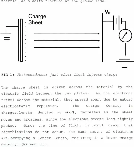
PROBLEM DEFINITION AND PHYSICAL DESCRIPTION
Figure 1 is a schematic of a photoconductor that has a
constant voltage at one plate and is grounded at the other
plate. The material receives energy from a light flash.
As a result of the energy input, a sheet of electrons is
injected at the ground side of the material. Initially the
sheet of electrons defines the charge density inside the
material as a delta function at the ground side.
Charge
Sheet
Vf
FIG 1: Photoconductor just after light injects charge
The charge sheet is driven across the material by the
electric field between the two plates. As the electrons
travel across the material, they spread apart due to mutual
electrostatic repulsion. The charge density in
charges/length, denoted by n(x,t) , decreases as the sheet
moves and broadens, since the electrons become less tightly
packed. Since the time of flight is short enough that
recombinations do not occur, the same amount of electrons
are occupying a longer length, resulting in a lower charge
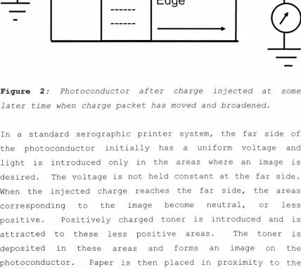
[image:12.490.27.460.215.719.2] [image:12.490.26.462.219.697.2]Figure 2 illustrates the charge packet widening as it moves
across the material. Since the total number of charges in
the packet remains constant while inside the material, the.
charge density, n(x,t) , decreases over time.
Charge
Packet
Figure 2: Photoconductor after charge injected at some
later time when charge packet has moved and broadened.
In a standard xerographic printer system, the far side of
the photoconductor initially has a uniform voltage and
light is introduced only in the areas where an image is
desired. The voltage is not held constant at the far side.
When the injected charge reaches the far side, the areas
corresponding to the image become neutral, or less
positive. Positively charged toner is introduced and is
attracted to these less positive areas. The toner is
[image:13.490.31.459.316.699.2] [image:13.490.37.458.499.715.2]photoconductor and by introducing a negative charge to the
back of the paper, the toner then gets drawn away from the
photoconductor and is deposited on the paper in the desired
image areas. After heating the paper and toner, usually
under pressure, the toner melts on and into the paper and a
ELECTRIC FIELD
For this one-dimensional problem, charge density, n(x,t) , is
the spatial derivative of the E-field. Poisson'
s equation
states that V'V= hi. Since this is
a one-dimensional
d2V dE(x,t)
problem, =kn{x,t)
, which is the one-dimensional
dx dx
version of Poisson' s equation V2V=
kn(x,t) with k = \.
E-field, which is the change in voltage/unit distance, is
constant before energy is introduced to the material.
After the sheet of electrons is injected, E-field becomes a
step function at the ground side of the material and the
original E-field is changed. Figure 3 illustrates this
behavior.
X
FIG 3: E-field before charge injection (a) and just after
charge injection (b) .
dV _
E-field is the spatial derivative of voltage, =
E(x,t) , and
ox-, x E(x,t)
n(x,t) = . Before the light flash, the voltage
drop ox
across the photoconductor is constant 4(a) and so E-field
is constant 4(b). There is no charge density. This
relationship is shown in figure 4 .
V
(a)
X
(b)
X
FIG 4: Voltage (a) and E-field (b) before charge injection.
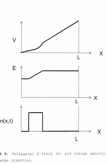
After the electrons are injected and have traveled across
the material for some time, the voltage drop is not a
linear function anymore; it has become parabolic in the
region of the charge as in figure 5(a). The E-field is
changed; its graph in figure 5(b) has a constant slope in
the region of the charge. Outside the charge area, the
[image:16.490.57.456.54.690.2]spread from the initial delta function and the charge
density is lower.
V
>
X
A
A\
n(x,t)
L
L
*
X
*
X
FIG 5: Voltage (a) E-field (b) and charge density (c) after
[image:17.490.47.390.86.612.2]Note that voltage is the integral of E-field with respect
to position between the two plates of the photoconductor
and is constant since the total change in voltage is
constant. This relationship is represented by the equation
_.
MATHEMATICAL DESCRIPTION
When the charges are contained within the photoconductor
material, the number of charges between the plates is given
by the equation:
L
I n(x,t)dx=number
ofcharges o
The instantaneous change over time in the number of charges
in, a small region, Ax, is given by,
i, .'
(n(x,t)Ax)=
-(p(E(x,t))E{x,t)(n(x +Ax,t)-n(x,/))
where p(E(x,t))E(x,t) is the average velocity of the charges.
Qividing both sides by Ax and rearranging, the result is
the conservation law:
^^
+|-
p(E(x,t))E(x,t)n(x,t)=0(
1)
dt ox
When some charges reach the far side of the photoconductor,
an external current occurs. The total electrostatic force
on a charge depends on the location and velocity of the
charge. (Feynman [2]). The current density, j in
charge/mic2-msec, moves through a surface that is
perpendicular to current flow.
Current density, j, is equal to charge density times
velocity, n(x,t)V . Current is the integral of the normal
component of flow through all the elements of the surface and is represented by
_
=
where m is the unit vector normal to the surface. If there
is a net current out of a closed surface, the charge inside
must decrease by the same amount because of the
conservation of charge. Therefore
f
\.mds =(3)
The charge inside is equal to
[
ndx . Since j=V and theLength
average drift velocity is constant, applying the del
operator in the direction of current flow gives
<9n <9n dx dn dn dn ,A.
Vj=Vov = v= = or v = . (4)
dx dx dt dt dx dt
Velocity is the product of mobility and E-field;
V=
p(E(x,t))E(x,t) . Rearranging terms yields the same
conservation law as in the condition where where all the
charges are contained within the material:
<*^
+JLp(E(x,t))E(x,t)n(x,t)
=0dt dx
In Eq. (1), p(E(x,t)) is the mobility of the material, which
can be thought of as velocity/unit E-field. The
Poole-Frenkel equation states p(E{x,t)) =
p0e^E(xJ)
, where p0 and /3
are constants that are unique to the material.
(Borsenberger [11])
Since ^-=
n{x,t) , after integrating both sides of Eq.(i; dx
from zero to x with respect to x , the equation can be re
written as
^>+MWM<*,0^
=*>(5)
This equation can be integrated term-by-term with respect
to x from 0 to L, where L is the width of the
photoconductor material:
5 r
dt
\E(x,t)dx+
f
p(E(x,t))E(x,t)dx=c(t)L
{ dx
(6)
Since the integral of (x,r)with respect to x is V{t) , or
voltage, the equation then becomes:
d
-V{t)+
\p{E{x,t))E(x,t)dx
= Lc{t)dt
(7)
^ince voltage does not change with time the first term
drops out and the equation then reduces to:
dE
C OtL
p(E{x,t))E(x,t) dx= Lc(t) dx
(8)
Equation (5) is similar to a standard initial boundary
value problem for a hyperbolic conservation law:
^^
+p(E(x,t))E(x,t)^^-=0, 0<t, 0<x
W
dt dx
with the initial condition
and the boundary condition.
E(x,0)=
g(x)
dE
The problem for this project is similar to the above but
has an extra unknown, c(t) , and an extra non-local condition.
The result is this problem, which appears to be well posed:
dE(x^+p(E(x,t))E(x,t)^^-
=c(t), 0<t, 0<x
dt dx
with initial condition:
and the boundary condition:
and the extra non-local condition :
E(x,0)=
g(x)
dF
(0,0=
c(0 dt
\L
MOTIVATION FOR USING METHOD OF CHARACTERISTICS
This problem is best solved using the method of
characteristics. Finite difference and finite element
methods work well with smooth functions, but this function
is not smooth. Finite difference and finite element
methods would set up a grid for time and space and try to
break the wave into spatial increments and treat the entire
E-field as a function of position at each time step.
Because the initial E-field is a step function, no matter
how large or small the pieces of E-field are sliced, Axis
zero initially. The derivative of E-field with respect to
position using these initial values is undefined and charge
density is a delta function. Ax changes over time as the
charges spread out and cannot be quantified. The method of
characteristics uses the change in x with respect to time
to determine characteristic curves. Then along the curves,
E-field changes linearly with respect to time. The error
using finite difference and finite element methods is
proportional to
d2V dn
dx2
dx
=charge density.
Initially, charge density is a delta function at the ground
plate, which would make the error large and the error bound
infinite using finite difference or finite element methods.
The method of characteristics looks at pieces of charge
only within the charge packet, on the characteristics, and
solves each section independently over time. Outside of the
charge packet we know that the charge density is zero and
METHOD OF CHARACTERISTICS: MATHEMATICAL DETAILS
By using the method of characteristics, we reduce the
original partial differential equation to a large system of
ordinary differential equations with t as the independent
variable. We define characteristic curves, along which the
E-field changes only with respect to time. The slopes of
these characteristic curves equal the velocities of the
charges as they travel through the material. On the
characteristic curves the PDE for E-field reduces to an
ODE.
In equation 8 we solved for c(t)
1 c(t)=
L
}Moe E-dx
E{x=L)
p0 \EeprEdE
(.v=0l
If we make the substitution,
u = 4e
the equation becomes
(t) = j[p0J2u3e^"du
Integration by parts results in
*>-t
-l^"j+6u-3/3u2+/32u3
_Ml
L
(10)
2
+6U-3/?2+V
(H)
We then define the characteristic curves by,
dx
dt
(12)
Along these characteristic curves,
dE dE dxdE dE ^dE , .
= + = +pE =
c{t) dt dt dt dx dt dx
Then along such a curve,
dE
dt L
2 eprE
J__.+6w_3/?
u2 p2 3Ai/rar/)
KUnill)
(14)
The problem defines a rarefaction wave; the characteristic
curves do not intersect because their slopes increase as a
function of mobility and E-field.
The system of differential equations to be solved is then:
f
=pE,=p0e^E,
dE;
dt
1 2
-efiJI{-+6^E-3/3E+
'\
0<x<LL/33
p 1"""
L fi- P
+
k
"k-L -x,
k
\xk~ xk-\J
I, xk>L
8Ej ~dt (0,t)
= c(t)
Ei(x,0)=V(t>
L
J E(x,t)dx=V(t)--0
_______ L
SOLUTION
To solve the system of ODEs, we used Matlab's ODE45 Solver,
which integrates the individual differential equations over
time simultaneously. This solver uses a Runga-Kutta 4-5
method with variable time step. The output was set for
evenly spaced time intervals.
By solving for E-field over time with a range of mobility
values, results can be compared to measured current and
time of flight to determine the mobility that matches the
measured results.
In this project, the parameters varied were: amount of
initial E-field displacement caused by charge injection,
and the mobility constants pQ and P . The program was run
initially with nominal values of p0=
(1 . 0micron2/volt-msec)
and P=
(0 . 0 0 1 5-JprnI V ) , and an E-field displacement from
20V/micron to OV/micron at the ground side. The ranges for
the variable changes are shown in Table 1:
Sample Initial
E-high
V/mic
Initial
E-low
(V/mic)
^0
(micron'/volt-msec)
P
(jpm/V )
1 20 0 1.0 0.0015
2 20 10 1.0 0.0015
3 20 0 1.0 0.02
4 20 0 1.2 0.0015
[image:26.490.31.462.67.698.2]Mobility was increased slightly by changing p from 0.0015
to 0.02 with very little change in the duration of time of
flight or the magnitude of E-field during that time. Much
larger changes in /? would be necessary change mobility
enough to see much of a difference in behavior. p0 was
then changed from 1.0 to 1.2, creating a larger change in
mobility, and creating a greater change in response. The
time of flight decreased as expected with higher mobility,
and the charges spread more as their movement within the
material was less restricted.
RESULTS & CONCLUSIONS
Using the method of characteristics, the initial partial
differential equation was reduced to a system of ordinary
differential equations. This system of ODEs was then
solved numerically using Matlab' s ode45 solver.
As expected, when mobility values increase, the time it
takes the charge packet to reach the far side of the
photoconductor is reduced. As more energy is introduced
resulting in a larger disturbance of E-field, the time for
the packet to travel to the other side increases. When
less energy is introduced, the packet takes less time to
travel across, and does not broaden as much since there are
SUMMARY
For this problem E-field can be determined at any position
and time by solving the PDE with the method of
characteristics. Mobility can be inferred by looking at a
range of solutions for various mobilities and finding a
match with measured experimental values. Further
research
on this problem might include:
Looking at materials that are not homogeneous
Looking at the problem in 2 or 3 dimensions
ACKNOWLEDGEMENTS
At this time I would like to acknowledge the many people
who have contributed in so many ways to make this project
possible. First, many thanks to my committee of Dr.
Bautista, Dr. Diute, and Dr. Ross for their help, guidance,
and encouragement along the way. Thank you to everyone in
the Department of Mathematics and Statistics for all the
help and for making this program possible, especially Dr.
Maggelakis and Dr. Shahmohamad. Thank you to former
colleague from Xerox, Dr. Surendar Jeyadev, for bringing
this problem to my attention and for meeting with my
committee to explain the details. Thank you also to other
former Xerox co-workers, Dr. James Feng and Shawn Rowan for
their help along the way in clarifying certain details and
concepts. Finally thank you to Denise Lake and Andrew
APPENDIX
ASAMPLE
RESULTS
SAMPLE 1
Nominal Conditions
Resultswith p0 =1 micronsVV-msec and /?= .0015
Initial E fieldaftercharge injection0-20 V/msec
E fieldandChargeDensityatinitial, 1/4, 1/2, 3/4,andtotalof2.5msec
40i i40i 140i 140, ,40i
0 10 20 0 10 20 0 10 20 0 10 2D 0 10 2D
4U 4U 4U 40 40
30 30 30 30 30
20 20 20 20 2D
10
n
10
n i . i . 10
n " 1 10
0
10
n
[image:30.490.82.411.144.392.2] [image:30.490.41.411.426.700.2]0 10 20 0 10 20 0 10 20 0 10 2D 0 10 2D
FIG. Al: E-fieldandChargedensityatseveraltimesteps as chargetravels
_ 1.5
-Characteristic Curves
10 15
X Position in Microns
20
FIG. Al.l: Thecharacteristic curvesform a rarefactionfan.
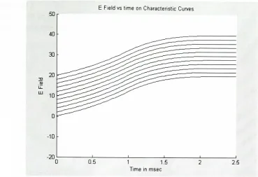
E FieldvstimeonCharacteristicCurves
1 1.5
Time inmsec
FIG. A1.2: The change in Efieldas afunction oftime isa constant which depends on
time. Therefore, at each timestep thechange inE-fieldis the same, resulting inparallel
[image:31.490.42.411.40.293.2]SAMPLE 2
Resultswith p0 =1 microns2/V-msec and /?= .0015
Initial Efieldaftercharge injection 10-20V/msec
E fieldandChargeDensityatinitial, 1/4, 1/2, 3/4,andtotalof2.5msec
40 40 , 40 40 : 40
20 20 20 20
-20 -20
--20---20 --20
0 10 20 0 10 20 0 10 20 0 10 20 0 10 20
40
30
20
10
0'f
40
30
20
-i 40
30
20
40
30
20
-40
30
20
10 10 10 10
0 -n 01 =
0 ___ n
[image:32.490.83.413.100.344.2]0 10 20 0 10 20 0 10 20 0 10 20 0 10 20
FIG A2: Less disturbance of initialEfieldresults in a shortertimeforcharges to move through thematerialthanFIG. Al. Mobilitycoefficients are same as FIGAl
CharacteristicCurves 2.5
<d 1.5
co
E
M 1
0.5
10 15
X Position in Microns
20 25
[image:32.490.72.415.355.624.2]E FieldvstimeonCharacteristic Curves
cu 50
40
30
20
10--10
-20
0.5 1 1.5
Timeinmsec
[image:33.490.47.411.39.294.2]2.5
FIG. A2.2: E-fieldchanges less as in time sincethere is less initialdisturbanceand the
SAMPLE 3
Resultswith p0=\.0 microns /V-msecand /?=0.02
Initial E field after chargeinjection 0-20 V/msec
E fieldandChargeDensityatinitial, 1/4, 1/2, 3/4,andtotalof2.5msec 40
r-40- -40
r--1 40 40, '
20 20 20 20
-20 !-20 -20 -20
0 10 20 0 10 20 0 10 20 0 10 20
40 40
30 30
20 20
10 10
0 C
0
) 10 20 Q[=
[image:34.490.66.411.51.335.2]0 10 20 0 10 20 0 10 20 0 10 20
FIG A3: Results are almost thesame as FIGAl since mobility is not changed much by
thischangein P
CharacteristicCurves
10 15
X Positionin Microns
20
FIG A3.1: Rarefaction fan is similar to nominal condition fan because change in
[image:34.490.36.420.367.706.2]E FieldvstimeonCharacteristicCurves
2
1 1.5
Time inmsec
FIG A3.2: Efieldshows similar chage as afunction oftimeas nominal conditions since
[image:35.490.69.409.37.288.2]SAMPLE4
Resultswith p0 =1
.2 microns2/V-msec and P =.0015
Initial E fieldafter chargeinjection 0-20V/msec
E fieldandChargeDensityatinitial, 1/4, 1/2, 3/4,andtotalof2.5msec
40 40 40 40 -i40
20 20 20 20
-20 -20 20 -20 -20
0 10 20 0 10 20 0 10 20 0 10 20 0 10 20
40
-40 40 40
30 30 30 30
20 20 20 20
10 10 10 10
0 I 0 0_ .. .
0
[image:36.490.80.414.71.334.2]0 10 20 0 10 20 0 10 20 0 10 20 0 10 20
FIG. A4: Mobilityincreasedbychanging p0from 1.0to 1.2
OtherM'ise initialconditions are thesame asFIG. Al. Increasein mobilityresults inless
timeforcharge toreach thefarsideofthephotoconductor. Chargesspread more
travelingacross material
2.5
1.5
E
H 1
0.5
Characteristic Curves
10 15
XPositionin Microns
20 25
[image:36.490.53.412.409.675.2]E FieldvstimeonCharacteristicCurves 50
40
30
20
CU
-10
-20
0.5 1 1.5 2 2.5
[image:37.490.82.411.60.324.2]Timeinmsec
APPENDIX B MATLAB CODE
Matlab's ODE solvers require an initial condition, the type
of solver to be used, the variable of integration, and a
function that defines the differential equations to be
solved. Since this problem is looking at pieces of the
charge sheet over time, each piece is solved for
individually.
Before the charge sheet is generated, the E-field is
constant and is equal to the known voltage divided by the
photoconductor width. After the light flash, the E-field
is disturbed at the ground-side of the material,
proportionally to the energy introduced. For initial
values, there are a set of zeros representing the ground
position for each piece of charge and a set of evenly
spaced values for E-field spanning the range achieved with
a known energy introduced. The initial values for the
solver are stored in an array containing values of zero for
x and a range of corresponding E values .
The solution at each time step is a row in the solution
matrix containing the next set of x values and E values.
After the initial condition, the E-field between the ground
side and the trail edge of the charge packet is the same as
the value at the trailing edge. Before the leading edge of
the packet reaches the charge side of the material, the
E-field between the leading edge and the charge side is the
When the trailing edge of the packet reaches the charge side, all the charges are neutralized and the E-field is back where it started before the introduction of energy.
Charge density is calculated by numerically taking the
derivative of E with respect to x.
The first file, proj .m, is the code to run the program. It
calls the ODE solver, creates initial values, and generates the output graphs. The second file, Projsol.m, defines the system of ODEs and integrates them for each time step.
M file proj .m
% Carol Panepinto MS Project August 2005
% This file contains the set of commands that defines initial
conditions in the matrix,
% calls the ODE solver, and generates the output graphs
o.
% clear variable values before running code
clear all
%initials: elements representing x when the charge is injected at time
zero
initials = zeros(1
, 201) ;
O o
%set up row vector for loop size
Q. "5
index = linspace(1,201,201);
o o
lenter values for initial E field range
highE = input('input highest initial value for E when charge is
% Set up loop to create the evenly spaced range of initial E values
for i = index
initials2(i) = lowE + i*
( (highE-lowE) /201); %initials2: elements representing E when the charge is injected
end
% combine initial x and E values into one column vector called inits Q
"5
inits=[initials, initials2] '
; % inits: initial x and E values
o
o
% input total time and calculate evenly spaced time steps for output
time = input('input total time for
the charges to travel in msec=? ') tspan =
linspace(0, time,100) ; %tspan: evenly spaced time
increments for output based on total time
% call the function solver using
% inputs of initial x and E and values and the tirnespan. store the output in a matrix called
% sol with a column of t(time) values and columns for the calculated x and E values
% each column of x and E values corresponds to one charge piece over time
[t,sol]=ode45(@Projsol, tspan, [inits]);
% retrieve values for last time step and plot x vs. E -fill in values after
% trail edge and before lead edge if necessary
figure(5)
hold on
soll00=[0 sol(100, 1:201) 25 sol(100,202) sol ( 100,202:402) sol(100,402) ] ;
subplot (2,5,5), plot (sol100(1:203),sol100(204:406))
% retrieve values for first time step and plot x vs. E-fill in values
after
% trail edge and before lead edge if necessary figure (5)
hold on
soll=[0 sol(l, 1:201) 25 sold,202) sol(1,202:402) sold,402)];
subplot (2, 5, 1) , plot (soil(1:203) , soil( 204:406) )
axis ( [0 25 -20 40] )
% retrieve values for 1/4 time and plot x vs. E-fill in values after
% trail edge and before lead edge if necessary figure (5)
hold on
i
sol25=[0 sol (25, 1:201) 25 sol(25,202) sol(25,202: 402) sol (25,402)] ; subplot (2, 5,2) , plot (sol25(1:203) , sol25 (204:406) )
axis ( [0 25 -20 40] )
% retrieve values for 1/2 total time and plot x vs. E-fill in values after
% trail edge and before lead edge if necessary figure (5)
hold on
sol50=[0 sol (50, 1:201) 25 sol(50,202) sol (50, 202:402) sol(50,402)] subplot (2,5, 3) , plot (sol50 (1:203) , sol50 (204:406) )
axis ( [0 25 -20 40] )
% retrieve values for first time step and plot x vs. E-fill in values after
% trail edge and before lead edge if necessary
figure(5)
hold on
sol75=[0 sol(75,1:201) 25 sol(75,202) sol(75, 202: 402) sol (75, 402) ] ,
[image:41.490.37.445.69.498.2]% set up index to plot position vs. time at some time steps
% to see some of the characteristic lines
index10=1 inspace(1,201, 11) ; for q = indexlO
% plot x vs. t to get dx/dt = mu*E figure(2)
hold on
plot (sol (:,q) , t) % plot x vs. t
axis ( [0 25 0 time] )
end
% set up index and plot time vs. E field at some time steps
% to see E field change over time on the characteristic curves
for r = indexlO
% plot t vs. E figure(4 )
hold on
plot (t, sol (:, (r+201) ) )
axis([0 time
lowE-(highE-lowE) highE+1.
5*
(highE-lowE) ] )
end
% Label Graphs o
o
figure(2)
xlabelf'X Position in Microns')
ylabel('Time in msec') title('
Characteristic Curves')
hold off
figure (4)
xlabel('Time in msec')
ylabel ('E Field'
)
title('E Field vs. time on Characteristic Curves'
hold off
% numerically calculate the derivative of E with respect to x to get
charge
% density at first time step
figure (5)
dE=diff (sol(2,202: 402) ) . /diff (sol (2,1:201) ) ;
[image:42.490.44.409.72.727.2]% set up matrix containing x values corresponding to positions
% between the photoconductor plates and charge density values with zero
% values outside the charge packet positions
dl=[0 xd(l) xd xd(200) 25 0 0 dE 0 0] ;
% Plot Derivative (Charge Density) vs. Position at initial time step
subplot (2,5,6), plot (dl (1:204) ,dl (205:408) )
axis ( [0 25 0 40] )
figure (5)
% numerically calculate the derivative of E with respect to x to get
charge
%i density at 1/4 way through total time
idE25=diff(sol (25,202:402) ) ./diff(sol(25, 1:201) ) ;
xd25=sol (25,2:201) ;
% set up matrix containing x values corresponding to positions
% between the photoconductor plates and charge density values with zero
% values outside the charge packet positions
d25=[0 xd25(l) xd25 xd25(200) 25 0 0 dE25 0 0];
% Plot Derivative (Charge Density) vs. Position 1/4 way through total
time
subplot(2,5,7), plot(d2 5 (1:204),d2 5 (205:408))
axis( [0 25 0 40] )
figure(5)
% numerically calculate the derivative of E with respect to x to get
charge
% density at 1/2 way through total time
dE50=diff (sol(50,202:402) ) . /diff(sol (50,1:201) ) ;
xd50=sol (50,2:201) ;
d50=[0 xd50(l) xd50 xd50(200) 25 0 0 dE50 0 0];
% Plot Derivative (Charge Density) vs. Position at 1/2 way through
time
subplot(2,5,8) , plot (d50 (1:204) , d50(2 05:408) )
axis( [0 25 0 40] )
figure (5)
% numerically calculate the derivative of E with respect to x to get
charge
% density at 3/4 way through total time
d75=[0 xd75(l) xd75 xd75(200) 25 0 0 dE75 0 0] ;
* Plot
Derivative (Charge Density) vs. Position at 3/4 way through
time
subplot(2,5,9), plot(d75(1:204),d75 (205:408) ) axis ( [0 25 0 40] )
% % % %calculate derivative of E with respect to x to get n at final time
% step
figure(5)
% numerically calculate the derivative of E with respect to x to get
charge
% density at final time step
dE500=diff (sol(100,202:402) )./diff(sol(100,1:201) ) ; xd500=sol(100,2:201) ;
d500=[0 xd500(l) xd500 xd500(200) 25 0 0 dE500 0 0];
% Plot Derivative (Charge Density) vs. Position at final time step subplot(2,5, 10), plot(d500 (1:204) ,d500(205:408) )
axis ( [0 25 0 40] )
% Label Large Graph containing subplots of E-field and
% charge density at different time steps
figure(5)
subplot(2,5,3)
title(['E field and Charge Density at initial, 1/4, 1/2, 3/4, and total of ' num2str(time) ,
'
msec'])
% make movie of E field vs. position at each time step
set(gca, 'nextplot' , '
replacechildren' )
for s=l:100
figure (6) ;
solmov=[0 soils,1:201) 25 sol(s,202) sol (s, 202:402) sol(s,402)]
plot(solmovd:203), solmov(204: 406) ) ;
axis([0 25 lowE-(highE-lowE) highE+ (highE-lowE) ] ) ;
xlabel('Position in Microns') ylabel('E-field Volts/Micron')
title(['E-field as Charges Move Over
'
num2str(time), '
msec'] EFrame(s)=getframe;
end
% Run Movie of E-field over all time steps
movie(EFrame, 1)
%. make movie of charge density vs. position at each time step
[image:44.490.34.448.386.689.2]for t=l:100 figure(7) ;
warning off MATLAB:divideByZero
dEmov=diff(sol(t,202: 402))./diff(sol (t, 1:201) ) ;
xdmov=sol (t,2 :201) ;
dmov=[0 xdmov(1) xdmov xdmov(200) 25 0 0 dEmov 0 0] ;
plot(dmov (1:204 ) ,dmov( 205:408) ) ; axis ([0 25 0 highE*2] ) ;
xlabel ('Position in Microns')
ylabel ('Charge Density Coulombs/Micron')
title(['
Density as Charges Move Over '
num2str (time) , '
msec'])
DenFrame (t)=getfrarae;
end
% Run movie of charge density at all time steps
movie(DenFrame, 1]
File Projsol.m
% Carol Panepinto MS Project August 2005
%This file defines the function that describes the derivatives with respect to time:
% dx/dt=mu*E,and dE/dt=c(t) It then stores
% the results of integration in a matrix called sol
function charge =
projsol2 (t, sol)
% L is the width of the photoconductor L=25;
% b is one of the constants of the material and muO is the other constant
% per the Poole Frenkel equation
b=.0015;
t
mu0=1.0;
% the following constants for the calculation of dE/dt are pre
calculated to
[image:45.490.33.437.12.722.2]cl=(-6)/b; % -6/b
c2=(-3)*b; %-3b
c3=bA2; %b"2
% set N initially equal to the index corresponding to the lead edge
% of the E field
N=402;
% set up loop to check for the first time x>L and if this occurs, % set the corresponding index for E equal to one less than the index
for E
% where x>L and call this index N
index3 =
[1:201] ;
for m=index3
if sol (m)>=L
N=m+201-1;
break
else
end
end
% set up an array containing dx/dt and dE/dt
% if N is less than or equal to the index for the first E
value (trailing edge),
% then the trail edge has gone past the width of the material
% let the x values continue but set the corresponding E values to zero
% since all charges are gone from the material
if N <= 202
charge=[[muO.* (sol(202:402) ) . *exp(b. *sqrt(sol (202:4 02)) ) ] ; [zeros (201, 1)
]] ;
% if N is greater than the index of the first E value(trail edge) and
less than
% the index of the last (lead edge) E value, this means that the lead
edge
% has entered the far side and the E field will be calculated for the
% charge area between the far side and the trail edge. Since N
corresponds
% to a region where x is slightly less than L, the short area between this
% charge area and the charge plate is added to what is calculated for the
% whole charge area with the derived equations. The rate of change in
% of the E field is constant at each time step
elseif N < 402 & N > 202
charge =
[ [muO. *
(sol ( 202:4 02) ) . *exp (b. *sqrt(sol( 202:402) ) ) ] ;
[ ( (mu0*exp(b*sqrt (sol(N) ) ) ) *
(sol (M)-sol (N-l) ) * (L-sol (M-201) ) / (sol (N-201)-sol
(N-202) ) ) /L+ (cO*
(exp(b*sqrt(sol (N) ) ) )* (cl+6*sqrt (sol
(N) )+c2*sol (N)+c3*sqrt (sol(N) "3) )
)-(cO* (exp(b*sqrt
(sol (202) ) ) )*
(cl+6*sqrt(sol(202) ) +c2*sol(202)+c3*sqrt (so 1(202)A3)));
( (mu0*exp(b*sqrt(sol(N) ) ) ) * (sol (N)-sol
(N-l) ) * (L-sol
(N-201) ) /(sol
(N-201)-sol
(N-202) ) ) /L+ (cO*
(exp(b*sqrt (sol (N) ) ) ) * (cl+6*sqrt (sol
(N) )+c2*sol (N)+c3*sqrt ('sol(N) A3) )
)-jc(5*
(exp(b*sqrt(sol (202))))* (cl+6*sqrt
(sol (202) )+c2*sol (2 02)+c3*sqrt(so l'(202) A3) ) ) ;
( (mu0*exp(b*sqrt(sol (N))))*(sol(N)-sol (N-l) ) *
(L-sol (N-201) ) /(sol
(N-201)-sol
(N-202) ) ) /L+(cO*
(exp(b*sqrt (sol(N) ) ) )* (cl+6*sqrt (sol
(N) )+c2*sol (N)+c3*sqrt (sol(N) A3) )
)-(cO*(exp(b*sqrt (sol (2
02) ) ) )* (cl+6*sqrt (sol
(202) )+c2*sol(202)+c3*sqrt (so l'(202)A3) ) ) ;
( (mu0*exp(b*sqrt (sol (N)) ) )* (sol (N)-sol
(N-l) )*(L-sol
(N-201) ) / (sol
(N-201)-sol
(N-202) ) )/L+ (cO*
(exp(b*sqrt (sol(N) )) ) * (cl+6*sqrt (sol
(N) )+c2*sol (N)+c3*sqrt (sol(N) A3) )
)-(cO* (exp(b*sqrt (sol (2
02) ) ) )*
(cl+6*sqrt (sol (202) )+c2*sol(2 02)+c3*sqrt (so
1(202)A3)));
( (mu0*exp(b*sqrt (sol(N) ) ) )*(sol
(N)-sol(N-l) )* (L-sol (N-201) ) / (sol
(N-201)-sol
(N-202) ) ) /L+ (cO*
(exp(b*sqrt (sol(N) ) ) )*
(cl+6*sqrt (sol (N) )+c2*sol (N)+c3*sqrt (sol(N)A3) )
)-(cO*(exp(b*sqrt (sol (202))))* (cl+6*sqrt (sol
(202) )+c2*sol(2 02)+c3*sqrt(so
1(202)A3) ) );
( (mu0*exp(b*sqrt (sol (N) ) )) *
(sol (N)-sol (N-l))*
(L-sol (N-201)) /(sol
(N-201)-sol
(N-202) ) ) /L+ (cO*
(exp(b*sqrt (sol (N) ) ) ) * (cl+6*sqrt (sol
(N) )+c2*sol (N)+c3*sqrt
(sol(N)A3) ) )-(cO*
(exp(b+sqrt (sol(202) ) ) ) * (cl+6*sqrt (sol
(202) )+c2*sol (202) +c3*sqrt(so 1(202)A3) ) );
( (mu0*exp(b*sqrt(sol(N) ) ) ) *
(sol(N)-sol(N-l) ) * (L-sol (N-201) )/
(sol(N-201)-sol
(N-202) ) ) /L+(cO* (exp(b*sqrt (sol
(N) ) ) ) * (cl+6*sqrt (sol
(N) )+c2*sol (N)+c3*sqrt
(sol(N)A3) )
)-(cO* (exp(b*sqrt (sol (202))))* (cl+6*sqrt (sol
(202) )+c2*sol (202)+c3*sqrt (so
1(202)A3) ) ) ;
( (mu0*exp(b*sqrt(sol(N) ) ) )* (sol (N)-sol
(N-l) ) * (L-sol (N-2
01) ) / (sol
(N-201)-sol
(N-202) ) ) /L+ (cO* (exp(b*sqrt
(sol (N) ) ) )* (cl+6*sqrt (sol
(N) )+c2*sol(N)+c3*sqrt
(sol(N) A3) )
)-(cO*
(exp(b*sqrt(sol(202))))*
(cl+6*sqrt(sol (202) )+c2*sol (202)+c3*sqrt(so
1(202)A3) ) ) ;
( (mu0*exp(b*sqrt(sol (N) ) ) ) * (sol (N)-sol (N-l
)) * (L-sol (N-201
(N-(cO*
(exp(b*sqrt(sol (202) ) ) )* (cl+
6*sqrt (sol (202) )+c2*sol (202)+c3*sqrt(so 1(202)A3)));
( (muO*exp(b*sqrt (sol(N) ) ) )*
(sol(N)-sol (N-l) ) * (L-sol
(N-201) ) /(sol
(N-201)-sol (N-202) ) )/L+(cO*
(exp(b*sqrt (sol (N) ) ) ) * (cl+6*sqrt
(sol (N) )+c2*sol (N)+c3*sqrt (sol (N) A3) ) )
-(cO*
(exp(b*sqrt(sol (202) ) ) ) *
(cl+6*sqrt (sol (202) )+c2*sol(202)+c3*sqrt(so
1 (202)A3) ) ) ;
( (mu0*exp(b*sqrt (sol(N) ) ) )*
(sol (N) -sol (N-l) ) *
(L-sol (N-201) )/(sol
(N-201)-sol
(N-202) ) )/L+(cO*
(exp(b*sqrt (sol(N) ) ) ) *
(cl+6*sqrt(sol (N) ) +c2*sol(N)+c3*sqrt (sol(N) A3) )
)-(cO*
(exp(b*sqrt (sol (202) ) ) ) *
(cl+6*sqrt(sol (202) )+c2*sol (202)+c3*sqrt(so 1(202)A3)));
( (mu0*exp(b*sqrt (sol(N) ) ) ) *
(sol (N)-sol (N-l) ) * (L-sol (N-2
01 ) ) /(sol
(N-201) -sol
(N-202) ) ) /L+ (cO* (exp(b*sqrt
(sol (N) ) ) ) *
(cl+6*sqrt (sol(N) ) +c2*sol(N)+c3*sqrt
(sol(N) A3) )
)-(cO*
(exp(b*sqrt(sol (202) ) ) ) * (cl+6*sqrt (sol
(202) )+c2*sol (202)+c3*sqrt(so 1(202)A3)));
( (mu0*exp(b*sqrt(sol (N) ) ) )*
(sol (N)-sol(N-l) ) *
(L-sol(N-201) )/ (sol
(N-201) -sol (N-202) ) )/L+(c0*
(exp(b*sqrt (sol (N) ) ) ) * (cl+6*sqrt (sol
(N) )+c2*sol (N)+c3*sqrt (sol(N)A3))
)-(cO*
(exp(b*sqrt (sol (202) ) ) )* (cl+6*sqrt
(sol(202) )+c2*sol(202)+c3*sqrt(so 1(202)A3)));
( (mu0*exp(b*sqrt (sol (N) ) ) ) * (sol
(N)-sol(N-l)) * (L-sol
(N-201) ) /(sol
(N-201)-sol (N-202) ) ) /L+ (cO*
(exp(b*sqrt (sol (N) ) ) ) *(cl+6*sqrt (sol
(N) )+c2*sol (N)+c3*sqrt (sol(N) A3) )
)-(cO*
(exp(b*sqrt (sol (202))))*
(cl+6*sqrt (sol(202) )+c2*sol (202)+c3*sqrt (so 1(202)A3)));
( (mu0*exp(b*sqrt (sol(N) ) ) ) *
(sol(N)-sol(N-l) ) * (L-sol (N-201) ) / (sol (N-201)-sol
(N-202) ) )/L+ (cO*(exp(b*sqrt (sol
(N) ) ) )*
(cl+6*sqrt (sol (N) )+c2*sol (N)+c3*sqrt
(sol(N) A3) )
)-(cO*(exp(b*sqrt (sol (2
02) ) ) ) *(cl+6*sqrt (sol
(202) )+c2*sol (202)+c3*sqrt (so 1(202) A3) ) );
( (mu0*exp(b*sqrt (sol(N) ) ) ) *
(sol(N) -sol(N-l) )* (L-sol(N-201) )/(sol (N-201)-sol
(N-202) ) ) /L+ (cO*
(exp(b*sqrt (sol (N) ) ) )* (cl+6*sqrt (sol
(N) )+c2*sol (N)+c3*sqrt
(sol(N)A3) )
)-(cO*(exp(b*sqrt (sol (202))))* (cl+6*sqrt (sol
(202) )+c2*sol(202)+c3*sqrt(so 1(202) A3) ) ) ;
( (mu0*exp(b*sqrt (sol (N) ) ) ) * (sol
(N)-sol(N-l) )* (L-sol(N-201) )/(sol (N-201)-sol
(N-202) ) ) /L+(cO* (exp(b*sqrt (sol
(N) ) ) ) *
(cl+6*sqrt (sol (N) )+c2*sol(N)+c3*sqrt
(sol(N) A3) )
)-(cO* (exp(b*sqrt (sol(202))))* (cl+6*sqrt (sol
(202) )+c2*sol(202)+c3*sqrt (so 1(202) A3) ) );
( (mu0*exp(b*sqrt(sol (N) ) ) )*(sol (N)-sol (N-l
) ) *
(L-sol (N-201) ) /(sol (N-201)-sol
(N-202) ) )/L+ (cO* (exp(b*sqrt
(sol (N) ) ) ) * (cl+6*sqrt (sol
(N) )+c2*sol(N)+c3*sqrt (sol(N) A3) )
)-(cO* (exp(b*sqrt (sol (202))))* (cl+6*sqrt
(sol (2 02) )+c2*sol (2 02)+c3*sqrt(so
1(202) A3) ) ) ;
(N-202) ) )/L+(cO* (exp(b*sqrt
(sol(N) A3) ) )-(cO*
(exp(b*sqrt (sol (202)
1(202) A3) ) ) ;
( (muO*exp(b*sqrt (sol (N
201)-sol
(N-202) ) ) /L+(cO* (exp(b*sqrt
(sol(N)A3) ) )-(cO*
(exp(b*sqrt(sol (202)
1 (202) A3) ) ) ;
( (mu0*exp(b*sqrt (sol (N
201)-sol
(N-202) ) ) /L+(cO*
(exp(b*sqrt
(sol(N) A3) ) )-(cO* (exp(b*sqrt
(sol(202)
l.'(202) A3) ) ) ;
{ (mu0*exp(b*sqrt (sol (N
2oi)-soi
<n-202) ) ) /L+(cO* (exp(b*sqrt
(sol(N) A3) ) )-(cO*
(exp(b*sqrt (sol(202)
1(202) A3) ) ) ;
( (muO*exp(b*sqrt(sol(N
201)-sol
(N-202) ) )/L+(cO* (exp(b*sqrt
(sol(N) A3) ) )-(cO*
(exp(b*sqrt (sol(202)
1(202)A3) ) );
( (mu0*exp(b*sqrt (sol (N
201)-sol
(N-202) ) ) /L+(cO*
(exp(b*sqrt (sol(N) A3) )
)-(cO*
(exp(b*sqrt (sol (202)
1(202) A3) ) ) ;
( (mu0*exp(b*sqrt (sol (N 201)-sol
(N-202) ) )/L+ (cO* (exp(b*sqrt
(sol(N)A3) )
)-(cO* (exp(b*sqrt (sol
(202)
1(202) A3) ) ) ;
( (mu0*exp(b*sqrt (sol (N
201)-sol
(N-202) ) )/L+ (cO* (exp(b*sqrt
(sol(N) A3) )
)-(cO* (exp(b*sqrt (sol
(202)
1(202)A3) ) );
( (mu0*exp(b*sqrt (sol (N 201)-sol
(N-202) ) ) /L+(cO* (exp(b*sqrt
(sol(N) A3) )
)-(cO* (exp(b*sqrt (sol
(202)
1 (202) A3) ) ) ;
( (mu0*exp(b*sqrt (sol (N 201)-sol
(N-202) ) ) /L+(cO*
(exp(b*sqrt
(sol(N) A3) )
)-sol (N) ) ) )* (cl+6*sqrt
(sol (N) )+c2*sol (N)+c3*sqrt
) )*
(cl+6*sqrt (sol (202) ) +c2*sol (202)+c3*sqrt (so
) ) )*
(sol(N)-sol (N-l) )* (L-sol (N-201) ) / (sol
(N-sol (N) ) ) ) *
(cl+6*sqrt (sol (N) )+c2*sol (N)+c3*sqrt
) )*
(cl+6*sqrt (sol(202) )+c2*sol (2 02)+c3*sqrt (so
) ) )* (sol
(N)-sol(N-l) ) * (L-sol (N-201) )/(sol
(N-sol (N) ) ) ) * (cl+6*sqrt
(sol (N) )+c2*sol(N)+c3*sqrt
) )*
(cl+6*sqrt(sol (202) )+c2*sol (202)+c3*sqrt (so
) ) ) * (sol (N)-sol
(N-l) ) * (L-sol
(N-201) ) /(sol
(N-sol(N) ) ) ) *
(cl+6*sqrt (sol(N) ) +c2*sol (N)+c3*sqrt
) ) * (cl+6*sqrt
(sol(202) ) +c2*sol(202) +c3*sqrt (so
) ) ) * (sol
(N)-sol (N-l) )* (L-sol(N-201) )/(sol
(N-sol (N) ) ) ) * (cl+6*sqrt (sol(N) )+c2*sol (N)+c3*sqrt
) )*(cl+6*sqrt (sol
(202) )+c2*sol(202)+c3*sqrt (so
))) * (sol
(N)-sol(N-l) ) * (L-sol(N-201) ) /(sol
(N-sol(N) ) ) ) * (cl+6*sqrt (sol
(N) )+c2*sol (N)+c3*sqrt
) ) * (cl+6*sqrt (sol
(202) )+c2*sol(202)+c3*sqrt (so
) ) ) * (sol
(N)-sol(N-l) ) * (L-sol(N-201) ) / (sol
(N-sol (N) ) ) )* (cl+6*sqrt (sol (N) )+c2*sol (N)+c3*sqrt
) ) * (cl+6*sqrt (sol
(202) )+c2*sol (202)+c3*sqrt (so
) ) )*
(sol (N)-sol(N-l) )* (L-sol
(N-201) ) / (sol
(N-sol (N) ) ) ) * (cl+6*sqrt (sol(N) )+c2*sol(N)+c3*sqrt
) ) * (cl+6*sqrt (sol
(202) )+c2*sol(202)+c3*sqrt (so
) ) )* (sol (N)-sol
(N-l) )* (L-sol (N-2
01) )
/(sol(N-sol (N) ) ) )* (cl+6*sqrt (sol
(N) )+c2*sol (N)+c3*sqrt
) ) * (cl+6*sqrt (sol
(202) )+c2*sol(202)+c3*sqrt(so
))) *(sol
(N)-sol(N-l) ) * (L-sol (N-201) )/ (sol
(N-sol(N) ) ) ) * (cl+6*sqrt (sol
(N) ) +c2*sol(N)+c3*sqrt
( (muO*exp(b*sqrt (sol (N)) ) )* (sol
(N)-sol(N-l) )*(L-sol(N-201) ) / (sol
(N-201)-sol
(N-202) ) )/L+ (cO*
(exp(b*sqrt (sol(N) ) ) ) * (cl+6*sqrt
(sol (N) )+c2*sol(N)+c3*sqrt (sol (N)A3) ))
-(cO*
(exp(b*sqrt (sol (202) ) ) )*
(cl+6*sqrt(sol (202) )+c2*sol ( 202)+c3*sqrt(so
1(202)A3)));
( (mu0*exp(b*sqrt (sol(N) ) ) ) * (sol
(N)-sol(N-l) ) * (L-sol (N-201) ) / (sol
(N-201)-sol
(N-202) ) ) /L+(cO*
(exp(b*sqrt (sol(N) ) ) ) *
(cl+6*sqrt(sol(N) )+c2*sol (N)+c3*sqrt
(sol(N) A3) ) )-(cO*
(exp(b*sqrt (sol (202))))* (cl+6*sqrt
(sol(202) )+c2*sol (202)+c3*sqrt(so
1(202)A3)));
( (mu0*exp(b*sqrt (sol(N) ) ) ) *
(sol (N)-sol (N-l)) *
(L-sol(N-201) ) /(sol (N-201)-sol
(N-202) ) )/L+ (cO*
(exp(b*sqrt(sol (N) ) ) ) * (cl+6*sqrt
(sol (N))+c2*sol(N) +c3*sqrt
(so
vsqrt
so
(sol (N)A3) ) )-(cO*
(exp(b*sqrt (sol(202))))*
(cl+6*sqrt (sol (202) )+c2*sol (202)+c3*sqrt 1(202)A3)));
( (mu0*exp(b*sqrt(sol (N) ) ) )*(sol
(N)-sol(N-l) )* (L-sol (N-201) ) /(sol
(N-201)-sol
(N-202) ) ) /L+ (cO*
(exp(b*sqrt (sol(N) ) ) ) *
(cl+6*sqrt (sol (N) ) +c2*sol(N)+c3*sqrt (sol(N) A3) )
)-(cO*
(exp(b*sqrt(sol (202) ) ) )* (cl+6*sqrt (sol
(202) )+c2*sol(202)+c3*sqrt(so
1(202)A3) ));
( (mu0*exp(b*sqrt(sol (N) ) ) )* (sol
(N)-sol (N-l) )* (L-sol(N-201) ) /(sol (N-201)-sol
(N-202) ) )/L+(c0*(exp(b*sqrt(sol(N) ) ) )*(cl+6*sqrt (sol
(N) )+c2*sol(N)+c3*
(sol(N) A3) ) )-(cO*
(exp(b*sqrt (sol (202) ) ) )*(cl+6*sqrt
(sol(202) )+c2*sol(202)+c3*sqrt 1(202) A3) ) ) ;
( (mu0*exp(b*sqrt (sol(N) ) ) ) *
(sol(N)-sol (N-l)) *(L-sol (N-201
)) /
(sol(N-201)-sol
(N-202) ) )/L+ (cO* (exp(b*sqrt (sol
(N) ) ) ) *
(cl+6*sqrt (sol (N) )+c2*sol (N)+c3*sqrt
(sol(N) A3) )
)-(cO* (exp(b*sqrt (sol (2
02) ) ) )* (cl+6*sqrt (sol
(202) )+c2*sol (202)+c3*sqrt (so
1(202)A3) ) );
( (mu0*exp(b*sqrt (sol(N) ) ) ) * (sol
(N)-sol(N-l) )* (L-sol (N-201 201)-sol
(N-202) ) ) /L+(cO* (exp(b*sqrt (sol
(N) ) ) ) *
(cl+6*sqrt(sol (N))+c2*sol(N)+c3*sqrt
(sol(N) A3) )
)-(cO* (exp(b*sqrt (sol(202))))* (cl+6*sqrt (sol
(202) )+c2*sol(202)+c3*sqrt(so
1(202) A3) ) ) ;
( (mu0*exp(b*sqrt (sol (N) ) ) ) *
(sol (N)-sol (N-l) )* (L-sol (N-201) ) /(sol(N-201)-sol
(N-202) ) ) /L+(c0* (exp(b*sqrt (sol
(N) ) ) ) * (cl+6*sqrt (sol
(N) )+c2*sol (N)+c3*sqrt
(sol(N) A3) )
)-(cO* (exp(b*sqrt (sol (2
02) ) ) )*(cl+6*sqrt(sol
(202) )+c2*sol( 202 ) +c3*sqrt(so
1(202)A3) ) );
( (mu0*exp(b*sqrt(sol (N) ) ) ) * (sol (N)-sol (N-l
))* (L-sol (N-201
)) /(sol
(N-201)-sol
(N-202) ) )/L+(c0* (exp(b*sqrt (sol
(N) ) ) ) * (cl+6*sqrt (sol (N) )+c2*sol (N)+c3*sqrt (sol(N) A3) )
)-(cO* (exp(b*sqrt (sol (2
02) ) ) ) * 1 (202) A3) ) ) ;
.) ) /
(sol(N
-(cl+6*sqrt (sol (202) )+c2*
02) A3) ) ) ;
(mu0*exp(b*sqrt (sol (N) ) ) )* (sol )-sol
(N-sol(202)+c3*sqrt(so
. (N)-sol (N-l) )
* (L-sol
(N-201) ) /(sol(N
201)-sol
(N-202) ) )/L+(cO* (exp(b*sqrt
(sol (N
(sol(N) A3) )
(cO*
(exp(b*sqrt (sol(202))))*(cl+6*: 1(202)A3) ) );
sqrt (sol (202) )+c2*sol (202)+c3*sqrt (so
(muO*exp(b*sqrt (sol (N) ) ) )*
(sol (N)-sol (N-l) )* (L-sol (N-201) ) /(sol
(N-201)-sol (N-202) ) )/L+ (cO*
(exp(b*sqrt (sol (N) ) ) ) * (cl+6*
sqrt (sol(N) )+c2*sol(N)+c3* sqrt
(sol(N) A3) )
)-(cO*
(exp(b*sqrt (sol ( 202 ) ) ) ) *
(cl+6*
sqrt(sol (202) )+c2*sol (202)+c3*sqrt (so
K202)A3)));
( (mu0*exp(b*sqrt (sol (N) ) ) ) * (sol
(N)-sol (N-l) )* (L-sol (N-201) )
/(sol(N-201)-sol
(N-202) ) ) /L+ (cO*
(exp(b*sqrt(sol (N) ) ) ) * (cl+6*
sqrt (sol(N) )+c2*sol (N)+c3*sqrt (sol (N) A3) )
)-(cO*
(exp(b*sqrt (sol (202) ) ) ) * (cl+6*
sqrt (sol(202) )+c2*sol (202)+c3*
sqrt (so
1(202)A3)));
( (mu0*exp(b*sqrt (sol(N) ) ) ) *
(sol(N)-sol (N-l))* (L-sol
(N-201) )/(sol
(N-201)-sol
(N-202) ) ) /L+ (cO*(exp(b*sqrt
(sol (N) ) ) )* (cl+6*
sqrt (sol (N) )+c2*sol(N) +c3*sqrt
sqrt(sol (202) )+c2*sol (202)+c3*sqrt (so
N-l) ) *
(L-sol(N-201) )/ (sol
(N-ZUl)-SOI IIN
-202) ) ) /L+(cO*
(exp(b*sqrt (sol (N) ) ) )* (cl+6*
sqrt(sol(N) ) +c2*sol(N)+c3*sqrt (isol(N) A3) )
)-(cO*
(exp(b*
sqrt (sol (202) ) ) ) * (cl+6*sqrt (sol
(202) )+c2*sol(202)+c3*
sqrt(so 1 (202) A3) ) ) ;
( (muO*
exp(b*sqrt (sol (N) ) ) ) *
(sol(N) -sol(N-l) ) * (L-sol(N-201) ) /(sol
(N-201)-sol
(N-202) ) ) /L+ (cO*
(exp(b*
sqrt(sol(N) ) ) ) * (cl+6*
sqrt(sol (N) )+c2*sol (N)+c3*sqrt
(sol(N) A3) ) )-(cO*
(exp(b*
sqrt (sol(202))))*
(cl+6*sqrt (sol (202) )+c2*sol(202)+c3*sqrt (so
1(202)A3)));
( (muO*
exp(b*sqrt(sol (N) ) ) ) *
(sol (N)-sol(N-l) )* (L-sol(N-201) ) /(sol
(N-201)-sol
(N-202) ) )/L+(c0*
(exp(b*sqrt (sol (N) ) ) ) *(cl+6*
sqrt(sol (N) )+c2*sol (N)+c3*sqrt
(sol(N) A3) ) )-(cO*
(exp(b*
sqrt (sol(202) ) ) ) * (cl+6*
sqrt(sol(202) )+c2*sol(202)+c3*
sqrt (so 1 (202)A3) ) ) ;
( (muO*
exp(b*sqrt (sol(N) ) ) )*
(sol(N) -sol(N-l) ) * (L-sol(N-201) ) /(sol
(N-201)-sol
(N-202) ) ) /L+(cO*
(exp(b*
sqrt(sol (N) ) ) ) * (cl+6*
sqrt (sol(N) )+c2*sol (N)+c3*sqrt (sol(N) A3) )
)-(cO
'
.sdl(N)A3) )
)-(cO*
(exp(b*
sqrt (sol(202) ) ) ) * (cl+6* 1 (202)A3) ) ) ;
( (mu0*exp(b*sqrt(sol (N) ) ) )* (sol
(N)-sol (N-l) ) *
201)-sol
(N-N) "J) ) )
-exp(b*sqrt(sol(202) ) ) ) *(cl+6 1(202) A3) ) ) ;
sol (N)-sol(N-l) ) * (L-sol
(N-^u^; jj 1 1 ;
( (mu0*exp(b*sqrt (sol (N) ) 201)-sol
(N-sqrt (sol(202) )+c2*sol (202)+c3*
sqrt (so
(N-201) ) /(sol
(N-^U J.I-_4_l_
(141-202) ) )/L+ (cO*
(exp(b*
sqrt(sol (N) ) ) ) *
(cl+6*
sqrt(sol (N) )+
(sol(N)A3) )
)-(cO*
(exp(b*
sqrt(sol(202
sqrt
sqrt (so
sol (N-Hc2*sol(N)+c3
, , .
,
* (cl+6*sqrt (sol
(202) )+c2*sol (202) +c3*
1(202)A3) ) ) ; ( (muO*
exp(b*sqrt(sol(N) ) ) ) *
(sol(N)-sol (N-l)) * (L-sol (N-201
))/ (
201) -sol
(N-202) ) )/L+(cO*
(exp(b*
sqrt (sol(N) ) ) ) * (cl+6*sqrt(sol
(N) )+c2*sol(N)+c3*sqrt
(sol(N) A3) ) )-(cO*
(exp(b*
sqrt(sol (202) ) ) )* (cl+6*
sqrt (sol(202) )+c2*sol (202) +c3*sqrt (so 1(202) A3) ) ) ;
( (muO* (b*
sqrt (sol (N) ) ) )*
( (N) (N-l) ) * (L-sol(N-201
(N-202) ) )/L+(cO*
(exp(b*sqrt(sol
(N) ) ) ) * (cl+6*
sqrt (sol (N) )+c2*sol(N)+c3*sqrt
(sol(N) A3) ) )-(cO*
(exp(b*
sqrt(sol (202) ) ) ) * (cl+6*
sqrt (sol (202) ) +c2*sol (202)+c3*
sqrt (so
1(202) A3) ) ) ;
( (muO*
exp(b*sqrt(sol (N) ) ) )* (sol (N
)-sol (N-l) ) * (L-sol (N-2
01) ) / (sol (N-201)-sol
(N-202) ) )/L+(c0*
(exp(b*sqrt (sol (N) ) ) ) * (cl+6*
sqrt(sol(N) )+c2*sol (N)+c3*sqrt
(sol(N)A3) ) )-(cO*
(exp(b*
sqrt (sol(202) ) ) )* (cl+6*sqrt
(sol(202) )+c2*sol(202) +c3*sqrt(so
1(202)A3)));
( (muO*
exp(b*sqrt (sol (N) ) ) )* (sol (N)-sol
(N-l) )* (L-sol
(N-201) ) /(sol
(N-201)-sol
(N-202) ) ) /L+(c0*
(exp(b*
sqrt (sol (N) ) ) )* (cl+6*
sqrt (sol (N) )+c2*sol (N)+c3*sqrt
(sol(N) A3) ))-(cO*
(exp(b*
sqrt (sol (202))))*(cl+6*
sqrt (sol(202) )+c2*sol(202)+c3*
sqrt (so
1(202) A3) ) );
( (mu0*exp(b*sqrt (sol (N) ) ) ) *
(sol (N)-sol(N-l) ) * (L-sol(N-201) )/ (sol
(N-201)-sol
(N-202) ) ) /L+(cO*
(exp(b*
sqrt (sol(N) ) ))* (cl+6*
sqrt (sol(N) )+c2*sol (N)+c3*sqrt
(sol(N) A3) ) )-(cO*
(exp(b*
sqrt(sol (2 02) ) ) )* (cl+6*
sqrt(sol (202) )+c2*sol (202)+c3*sqrt(so
1 (202) A3) ) ) ;
( (mu0*exp(b*sqrt (sol (N) ) ) )*
(sol (N)-sol (N-l)) * (L-sol(N-201) ) / (sol
(N-201)-sol
(N-202) ) )/L+(cO*
(exp(b*
sqrt (sol(N) ) ) )* (cl+6*
sqrt(sol(N) )+c2*sol (N)+c3*sqrt
(sol(N) A3) ) )-(cO*
(exp(b*
sqrt(sol (202) ) ) ) *
(cl+6*
sqrt(sol (202) )+c2*sol (202)+c3*
sqrt(so
1(202) A3) ) );
( (muO*
exp(b*sqrt (sol (N) ) ) )*(sol (N)-sol (N-l
)) * (L-sol
(N-201) ) / (sol
(N-201)-sol
(N-202) ) )/L+(cO*
(exp(b*
sqrt (sol(N) ) ) ) * (cl+6*sqrt(sol
(N) )+c2*sol (N)+c3*sqrt
(sol(N) A3) ) )-(cO*
(exp(b*sqrt (sol (202))))* (cl+6*
sqrt(sol (202) )+c2*sol (202)+c3*
sqrt(so
1(202)A3) ) );
( (mu0*exp(b*sqrt (sol (N) ) ) )*
(sol (N)-sol (N-l) ) * (L-sol
(N-201) )/ (sol
(N-201)-sol
(N-202) ) ) /L+(cO*
(exp(b*sqrt(sol
(N) ) ) )* (cl+6*
sqrt(sol(N) )+c2*sol(N)+c3*sqrt
(sol(N) A3) ) )-(cO*
(exp(b*sqrt (sol
(202) ) ) ) *(cl+6*sqrt(sol
(202) )+c2*sol (202)+c3*
sqrt(so
1(202) A3) ) );
( (muO*
exp(b*sqrt (sol (N) ) ) )* (sol (N)-sol (N-l
))* (L-sol (N-201
))/ (sol
(N-201)-sol
(N-202) ) ) /L+ (cO*
(exp(b*
sqrt(sol (N) ) ) ) * (cl+6*
sqrt(sol (N) )+c2*sol (N)+c3*sqrt
(sol(N) A3) ) )-(cO*
(exp(b*sqrt(sol(202) ) ) )* (cl+6*
sqrt(sol (202) )+c2*sol (202)+c3*
sqrt (so
1(202)A3) ) ) ;
( (muO*
exp(b*sqrt (sol(N) ) ) )* (sol (N)-sol (N-l )) *
(L-sol(N-201) ) /(sol
(N-201)-sol
(N-202) ) ) /L+ (cO*
(exp(b*sqrt (sol
(N) ) ) ) * (cl+6*
sqrt (sol(N) )+c2*sol(N)+c3*sqrt
(sol (N)A3) )
)-(cO*
(exp(b*sqrt(sol (202))))* (cl+6*sqrt (sol
(202) )+c2*sol(202)+c3*
sqrt (so
1 (202) A3) ) ) ;
( (mu0*exp(b*sqrt(sol (N) ) ) )* (sol(N)-sol(N-l))* (L-sol
(N-201) ) /(sol
(N-201) -sol
(N-202) ) ) /L+(c0* (exp(b*
sqrt (sol (N) ) ) )* (cl+6*sqrt (sol
(N) )+c2*sol (N)+c3*sqrt
(sol (N)A3) )
)-(cO*
(exp(b*sqrt(sol (202) ) ) )*
(cl+6*
sqrt (sol (202) )+c2*sol(202)+c3*
sqrt(so
( (mu0*exp(b*sqrt (sol (N
201)-sol
(N-202) ) )/L+(cO*
(exp(b*
sqrt
(sol (N) A3) ) )-(cO*
(exp(b*
sqrt (sol(202)
1(202) A3) ) );
( (muO*exp(b*sqrt (sol (N
201)-sol
(N-202) ) ) /L+(cO*
(exp(b*sqrt
(sol(N) A3) ) )-(cO*