Application of the b-spline collocation method to a geometrically non-linear beam problem

Rochester Institute of Technology

RIT Scholar Works

Theses Thesis/Dissertation Collections

2-1-2010

Application of the b-spline collocation method to a

geometrically non-linear beam problem

Jason Magoon

Follow this and additional works at:http://scholarworks.rit.edu/theses

This Thesis is brought to you for free and open access by the Thesis/Dissertation Collections at RIT Scholar Works. It has been accepted for inclusion in Theses by an authorized administrator of RIT Scholar Works. For more information, please [email protected].

Recommended Citation

Application of the B-spline Collocation Method to a

Geometrically Non-Linear Beam Problem

By

Jason Magoon

A Thesis Submitted in Partial Fulfillment of the Requirement For Master of Science Degree in Mechanical Engineering

Approved by:

Dr. Hany Ghoneim - Thesis Adviser ________________________ Department of Mechanical Engineering

Dr. Steven Weinstein ________________________

Department Head of Chemical Engineering

Dr. P.Venkataraman ________________________

Department of Mechanical Engineering

Dr. Alan Nye ________________________

Associate Department Head of Mechanical Engineering

Department of Mechanical Engineering Rochester Institute of Technology

Permission to Reproduce the Thesis

Application of the B-spline Collocation Method to a

Geometrically Non-Linear Beam Problem

I, JASON MAGOON, hereby grant permission to the Wallace Memorial Library of Rochester Institute of Technology to reproduce my thesis in the whole or part. Any reproduction will not be for commercial use or profit.

Abstract

ACKNOWLEDGEMENTS

Above all, I would like to thank my wife, Jill, for her unwavering love, support and patience over the past 10 years of part time study. Without her encouragement and moral support, I would definitely not be a Masters of Science degree candidate.

I also would like to thank my grandmother, Harriet Schilling, for believing in me when nobody else in my life did. As a 16 year old high school drop out, I had very few options. She took me in and showed me that with hard work and determination, any goal is attainable.

I would sincerely like to thank Dr. Hany Ghoneim for his support, knowledge and extremely positive attitude. I am very grateful that he accepted my request and became my adviser for this research. Without his guidance and vision, this research project would not have turned out as well as it has.

Table of Contents

Abstract………...……..iii

Acknowledgements………....v

Table of Contents……….………….vi

List of Figures………..vii

List of Tables ………..…………viii

1 Introduction………...………… 1

2 B-spline Background…………...………..9

2.1 Introduction………...………..9

2.2 B-spline Curve Components………..11

2.2.1 Knot Vectors……….….…………12

2.2.2 Basis Functions……….……… 13

2.2.3 Control Points……….………..……… 18

2.3 Derivatives……… 20

3 One-Dimensional B-spline Collocation………...… 22

3.1 Example 1A……….. 24

3.2 Example 1B……….. 29

3.3 Example 2………. 39

3.4 Example 3………. 44

3.5 Discussion on Accuracy of B-spline Approximation…………... 51

4 Two-Dimensional B-spline Collocation………....…. 55

4.1 Example 4……….……… 58

4.2 Example 5……….……… 68

5 Non-Linear Beam Problem……….….…….. 78

5.1 Geometrically Non-Linear Beam Problem..………. 81

6 Conclusions and Discussion………92

List of Figures

Figure 1: Defining Polygon with Five Vertices……….……. 9

Figure 2: Basis Functions for k = 3………... 14

Figure 3: Basis Functions for k = 4………... 15

Figure 4: Basis Functions for the Interval: 2 1 0≤_t < _{………...… 16}

Figure 5: Basis Functions for the Interval: 1 2 1 < ≤_{t ……… 17}

Figure 6: Basis Functions for the Interval: 0≤_t<1_{……… 18}

Figure 7: Basis functions for third order B-spline approximation……… 25

Figure 8: B-spline solution plotted with the exact solution……….. 28

Figure 9: Basis functions for third order B-spline approximation with two intermediate Knot Vector points……….. 31

Figure 10: B-spline solution plotted with the exact solution……… 38

Figure 11: 5thOrderB-spline solution plotted with the exact solution……….………....38

Figure 12: B-spline solution plotted with the exact solution……… 42

Figure 13: 7thOrderB-spline solution plotted with the exact solution……….………....43

Figure 14: Euler-Bernoulli Beam Example Diagram……….….. 44

Figure 15: Basis functions for sixth order B-spline approximation……….. 45

Figure 16: B-spline solution plotted with the exact solution……….... 50

Figure 17: Plane Heat Transfer Problem……….. 58

Figure 18: Basis Functions for the ‘u’ Parameter………. 60

Figure 19: Basis Functions for the ‘w’ Parameter……… 60

Figure 20: 2-D B-spline Solution Contour Plot……… 66

Figure 21: ANSYS Solution……….…… 66

Figure 22: 2-D B-spline Solution Contour Plot for 5th Order Approximation…………..67

Figure 23: Plane Heat Transfer Problem……….. 68

Figure 24: 2-D B-spline Solution Contour Plot………..…….. 76

Figure 25: ANSYS Solution………. 77

Figure 26: Cantilevered Beam with vertical end loading……….…… 81

Figure 27: Basis functions for fourth order B-spline approximation with one Intermediate Knot Vector points……… 83

List of Tables

Table 1: Table of collocation points for Example 1a……….28

Table 2: Table of collocation points for Example 1b………37

Table 3: Table of collocation points for Example 2………..42

Table 4: Table of collocation points for Example 3………..50

Table 5: Over Damped Solution Comparison………51

Table 6: Over Damped Solution Time Comparison………..51

Table 7: Under Damped Solution Comparison for λ =2_……….52

Table 8: Under Damped Solution Comparison for λ =4_{………...…………. 53}

Table 9: Under Damped Solution Time Comparison for λ =4_{………….……….. 53}

Table 10: Under Damped Solution Comparison for λ =16_{………. 54}

Table 11: Under Damped Solution Time Comparison for λ =16_{………... 54}

Table 12: Ordinate Coordinates Calculated with Matlab ‘fsolve’ Command………….. 87

Table 13: Comparison of the B-spline solutions versus the Frisch-Fay solutions….…....89

Table 14: Ordinates Coordinates for Fifth Order B-spline………...……….89

Table 15: Comparison of the 5th Order B-spline solution vs. the Frisch-Fay solutions....89

1

Introduction

Engineers are researching solutions to resolve many of today’s technical challenges. Numerical techniques are used to solve the mathematical models in engineering problems. Many of the mathematical models of engineering problems are expressed in terms of partial differential equations. Two of the most popular techniques for solving partial differential equations are the Finite Element Method and the Finite Difference Method. The Finite Element Method involves dividing the domains into a finite number of sub domains called elements and placing nodes at predetermined locations around the elements boundary. The Finite Element Method finds the solution at each of the nodes very accurately. The elements, along with the nodes, form the mesh, which can be refined to provide any level of accuracy desired. An advantage of the Finite Element Method is that each element can have its own distinct geometry of varying complexities. This is extremely useful in solving complicated problems with unusual geometrical shapes or boundaries. Another one of the computational techniques used to solve mathematical models today is the Finite Difference Method. In the Finite Difference Method, a solution is derived at a finite number of points by approximating the derivatives at each of them. The accuracy of this method is based on the refinement level of the grid points where the solution is being evaluated.

that the B-spline Collocation Method procedure is simpler and easy to apply to many problems involving differential equations. This technique has been used in fluid flow problems with a great deal of success and more recently, some research has been conducted using the technique on computational aero acoustic [47] and biology [30] problems. However, for problems with complex geometries with curved boundaries, the Finite Element Method is still the computational technique of choice for most researchers.

This thesis explores the B-spline Collocation Method procedure in depth and lays the foundation for future research necessary to apply it to computational mechanics problems. In order to show the simplicity and accuracy of the B-spline Collocation Method, the deflection of a geometrically non-linear, cantilevered beam was calculated using the B-spline Collocation Method and compared to a known solution [10] found in the literature. To get to that point, a few steps needed to be completed.

1. The properties of B-spline curves and surfaces were thoroughly researched.

2. A thorough review of the research literature available for the B-spline Collocation Method, as well as, Geometrically Non-linear problems was conducted.

3. A comprehensive, step-by-step procedure was developed and extensively documented for applying the B-spline Collocation Method to the solution of Boundary Value problems.

4. A symbolic Matlab code was developed that can be easily extended to solve many Boundary Value problems.

deal of information on the properties of B-spline curves and surfaces was found in the Rogers [40], deBoor [6], Farin [9] and Prautzsch [35] books.

As stated previously, a great deal of research has been done in the past decade on applying the B-spline Collocation Method to fluid flow problems. A collocation method is based on evaluating the accuracy of a differential equation at a finite set of collocation points. This fluid flow research has yielded multiple methods for the determination of the collocation points. Fairweather and Meade [8] present a summary of the spline collocation methods for boundary value problems with an outstanding compilation of references. Their summary states that there are four types of spline collocation methods used in engineering research. They are:

1. Nodal which satisfies the differential equation at each distinct knot location (nodes) on which the spline is defined.

2. Orthogonal which satisfies the differential equation by collocating at the roots of orthogonal polynomials in each subinterval of the partition for which the spline is defined.

3. Extrapolated/Modified is a modified nodal method that achieves an optimal rate of convergence on a uniform partition.

4. Collocation-Galerkin combines the advantages of spline collocation with the advantages of the Galerkin finite element analysis methods [8].

points. The Gaussian points are the zeroes of the appropriate degree Legendre polynomials over the normalized knot interval. Johnson [18] compared using nodal and orthogonal collocation with nodal collocation at the Greville Abscissa points. He determined that using the Greville Abscissa was more convenient and did not result in a loss of accuracy. He also devised a method, called the Boundary Residual method [19], for including the pressure terms in the Navier-Stokes equation. Mazzia, Sestini and Trigiante [33] analyzed the convergence of multiple methods that have the collocation points coinciding with the knot points. This approach was validated by Saka and Dag [41], when they compared the B-spline results with the computed results of the Burgers’ equation and modified Burgers’ equation. Ramadan, El-Danaf and Alaal [36] use seventh order B-splines with collocation points uniformly distributed to solve the nonlinear Burgers Equation. Jator and Sinkala [17] devised a method where the collocation points form a strictly increasing sequence of points in the domain. Khattak and ul-Islam [26] compared the B-spline basis functions with a Radial basis function and had very similar results.

Another area where a much research has been done is mesh creation and refinement for two dimensional problems. Guzman and Morillo [13] use B-splines to define the domain of an unstructured mesh. Karim and Moser [43] defined an algorithm for two dimensional B-splines that allows the local refinement of the mesh in areas where it is required. Mesh refinement helps approximate the boundary layer of fluid flow problems by allowing an increase, or decrease if necessary, of node points in the region.

highest order differentials. This is a problem that arises in the boundary layer and therefore the boundary conditions cannot be satisfied in the governing differential equation. One of the more recent researchers, Kadalbajoo, et al, uses piecewise-uniform mesh points as collocation points. Kadalbajoo with Yadaw [20] used that collocation method to approximate a solution for a two parameter, singularly perturbed, convection-diffusion boundary value problem. With Kumar [21], Kadalbajoo used the same collocation strategy on a problem with an additional small delay factor. On another singularly perturbed convection-diffusion problem, Kadalbajoo, with coauthor Gupta [22] used that same piecewise-uniform mesh collocation strategy. Kadalbajoo and Arora [23] approximate the solution to a singularly perturbed problem by redefining the problem to include artificial viscosity, which is determined later. In order to solve a time dependant problem, Kadalbajoo, Awasthi and Gupta [24] use the piecewise-uniform collocation strategy on a singularly perturbed, linear convection-diffusion problem. Kadalbajoo and Aggaewal [25] approximate the solution of a self adjoint, singularly perturbed boundary value problem. To solve a problem that arises in biology, Lin, Li and Cheng [30] use B-splines to solve a singularly perturbed boundary value problem, with the use of wavelet functions. Rao and Kumar [37] used an optimization technique to select collocation points on a self adjoint, singularly perturbed boundary value problem. They compared a third order with two intermediate points with a solution from a paper using a seventh order smooth B-spline. Using a nodal collocation scheme, Rao and Kumar [38] also approximated the solution of a self adjoint, singularly perturbed boundary value problem in the space of an exponential B-spline.

placed arbitrarily, which allows them to avoid using mapping functions currently used in Computational Aero-Acoustics. Ghoneim [11] applies the B-spline collocation method with the smoothest open-uniform knot vector, orthogonal collocation points and Greville Abscissa for the control points to get the solution for the axial stretching of a composite hyperbolic structure. Ghoneim and Santos [12] applies the same method to approximate the axial stretching of a composite barrel shaped shell structure. Hou, Yin and Wang [14] applied the B-spline collocation method, using equal distance nodes as collocation points, to a variable thickness conical shell. Wu, Chung and Huang [49] use a Radial Spline Collocation method that does not require the collocation points to be equally spaced. This increases the accuracy when there are discontinuities in the load distribution, geometry or material properties of the beam. Sun [44] uses orthogonal, cubic, B-spline collocation for solving the equations of linear elasticity

One of the contributions of this thesis was to thoroughly document the B-spline Collocation Method in a very simple and easy to follow format. The example problems were solved in a step by step manner that any individual studying engineering or mathematics can follow and use the same technique to solve additional problems. The other contribution of this thesis was to apply the B-spline Collocation Method to solve a geometrically nonlinear beam problem. This will eliminate the need for the use of the elliptical integrals, which can be difficult to work with, in the solution of the large deflection problem. The work of Johnson [18], utilizing the Greville Abscissa as collocation points, is expanded upon and shown to be a far simpler approach than the elliptical integrals approach.

solution by Fay [10], in Chapter 2 of his book ‘Flexible Bars’. In his solution, Frisch-Fay goes through a very complex process to reach his solution. The B-spline solution developed here is found to be very accurate and far simpler to solve.

2

B-spline Background

2.1 Introduction

A spline is a continuous piecewise curve used to approximate a solution to a mathematical problem. A spline curve is dependant upon a relationship between the basis function and the vertices of a defining polygon. The B-spline curve has its own type of basis function, known as the B-spline basis, to establish the relationship with the defining polygon.

That relationship for the B-spline curve, P (t), is defined by the equation

∑

+

=

= 1

1

, ( ) )

(

n

i

k i iN t

B t

P ,

where B are the position vectors of the n + 1 defining polygon vertices and _i N_i,k(t) are the

normalized basis functions. The order ‘k’ of the basis function results in a polynomial of

degree, n, where n = k - 1. This equation will be discussed in detail later in the chapter. One

property of the B-spline curve is that it must lie entirely within the convex hull of the

defining polygon, as shown in Figure 1.

Other types of splines are used in the mathematical and engineering fields. Another

popular type of spline, the Bezier spline, uses the Bernstein basis function to establish the

relationship. However, the B-spline basis function has a few advantages over the Bernstein

basis function. One advantage is that the order (k) of the basis function can be reduced,

resulting in a curve with a lower degree (k-1), without affecting the approximations accuracy.

This can be accomplished by changing the number of vertices in the defining polygon with

the addition of intermediate points to the knot vector. Another advantage is that the B-spline

curves behave in a non-global manner, with each vertex, Bi, associated to a unique basis

function. This means that each vertex affects only the shape of the curve over a range of

values where the basis function has a value greater than zero. That behavior is helpful when a

local refinement to the function is necessary.

Some very important properties of the B-spline curve that will help solve and

troubleshoot problems are:

• P(t) is a polynomial of degree k – 1 on each interval x_i ≤t< x_i+1

• P(t) and its derivatives of order 1,2 ,…,k – 2 are all continuous over the entire curve

• The sum of the B-spline basis functions for any parameter value ‘t’ can be shown to

be ( ) 1

1

1

, ≡

∑

=

n

i k i t

N

• Each basis function is positive or zero for all parameter values

• Except for k=1 each basis function has one maximum value

• The maximum order in the smoothest of the curves is equal to the number of defining

polygon vertices

• The curve does not oscillate about any straight line more often than its defining

• The curve generally follows the shape of the defining polygon

• The curve is transformed by transforming the defining polygon vertices

• The curve lies within the convex hull of its defining polygon

• Ck-2 continuous at each transition point, called knot points, and Ck-1 continuous

elsewhere

2.2

B-spline Curve Components

In order to calculate B-spline curves three things are required:

1. Knot Vectors.

2. Basis Functions.

3. Control Points.

Once the knot vector is selected and the basis functions and control points are

calculated, the B-spline curve can be derived. The resulting B-spline curve, P(t)

approximates the solution to a predefined boundary value problem that can be locally

controlled by the location of the vertices of the defining polygon. The B-spline curve is given

by the equation:

∑

=

= 1

1

, ( ) )

(

n

i

k i iN t

B t

P t_min ≤t <t_max, 2≤k≤n+1 (1)

where Bi are the position vectors of the n + 1 defining polygon vertices. In the B-spline curve

calculation, the basis functions that are used are only the ones that represent the highest

order, k. A typical expansion of a third order, (k = 3) B-spline curve would look like this:

∑

=

= 1

1

, ( ) )

(

n

i

k i iN t

B t

P

) ( )

( )

( )

(t B₁N_1,3 t B₂N_2,3 t B₃N_3,3 t

2.2.1 Knot Vectors

The selection of the knot vectors is very important to the creation of the B-spline.

Their selection determines the order of the resulting polynomial and the size of intervals that

each B-spline basis function represents. In addition, the smoothness of the curve is

determined by the choice of the knot vector. The knot vector chosen must provide sufficient

resolution to approximate the solution of the mathematical problem.

There are 3 different types of knot vectors used. They are:

1. Uniform: Individual knot values are evenly spaced.

2. Open-Uniform: Multiplicity of knot values at ends equal to the order of the

B-spline curve and internal knot values are evenly spaced.

3. Non-Uniform: Unequally spaced and/or multiple internal knot values.

In this thesis, open-uniform knot vectors are used exclusively to calculate B-spline curves

and basis functions. The number of control points and basis functions when the open-uniform

knot vector is used is equal to (k + m), where ‘k’ is the order and ‘m’ is the number of

internal points in the knot vector. When there are no internal knot points, the B-spline basis

reduces to the Bernstein basis, rendering the smoothest curve. In this special case, the

resulting B-spline curve is a Bezier curve. Some examples with the corresponding order (k)

and number of internal points in the knot vector (m) are;

[0 0 0 1 1 1] k = 3, m = 0

[0 0 0 1 2 2 2] k = 3, m = 1

[0 0 0 0 1 1 1 1] k = 4, m = 0

[0 0 0 0 1 2 3 3 3 3] k = 4, m = 2

In order to make the algorithm simpler and faster to solve, they also can be

components of the vector by the largest value ‘h’ in the knot vector. However, note that this

normalization will have to be accounted for in the collocation process.

Example: [0 0 0 1 2 2 2] h = 2, k = 3

[0 0 0 ½ 1 1 1] Normalized

2.2.2 Basis Functions

Once the knot vector has been selected, the B-spline basis function can be calculated.

The B-spline basis functionNi,k(t) is defined by a recursive relationship that is known as the

Cox-deBoor recursion formula.

otherwise x t x t

N_i,1 i i 1

0 1 )

( ≤ < +

  

= (2)

1 1 , 1 1

1 , ,

) ( )

( ) ( ) ( ) (

+ +

− + +

− +

−

− − +

− − =

i k i

k i k i

i k i

k i i k

i

x x

t N t x x

x

t N x t t

N (3)

Where ‘i’ is a counter and ‘k’ is the order of the basis function. The values of xi are elements

of the predetermined knot vector that satisfies the relationshipxi ≤ xi+1. The basis functions

and the knot vector are defined in terms of the parameter ‘t’, which is a coordinate in

parametric space and may or may not coincide with any of the Cartesian coordinates. The

parameter t will vary from tmin to tmax along the B-spline curve. Also during calculation, the

convention of 0/0 = 0 must be adopted for the recursion to work. Their calculation is

completely driven by the predetermined knot vector. The order (k) of the basis functions

corresponds to an approximating B-spline polynomial of (k-1) degrees.

Here is an example for the following knot vector [0 0 0 1 1 1], with k = 3, using the

otherwise x t x t

N_i,1 i i 1

0 1 )

( ≤ < +

   =

1 1 , 1 1

1 , ,

) ( )

( ) ( ) ( ) (

+ +

− + +

− +

−

− − +

− − =

i k i

k i k i

i k i

k i i k

i

x x

t N t x x

x

t N x t t N

0 ) (

1 , 1 t =

N ; N_2,1(t)=0; N_3,1(t)=1; N_4,1(t)=0;

0 ) (

2 , 1 t =

N ; N2,2(t)=1−t; N3,2(t)=t; N4,2(t)=0;

2 3

,

1 (t) (1 t)

N = − ; N_2,3(t)=2t(1−t); 2 3

, 3 (t) t

N = ; N_4,3(t)=0

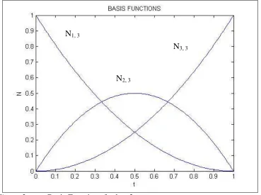
By plotting all three of the k = 3 basis functions, which are shown in Figure 2, a great

deal of information can be derived. Notice that at any value of t, the sum of all of the basis

functions is equal to a value of one. Also notice the degree of the basis function curves. The

curves of these basis functions are 2nd degree, which corresponds to the 3rd order B-spline.

Another property to observe is that the first basis function,N_1,k(t), always starts at a value of

one and ends at a value of zero, for the functions with no intermediate points in the knot

vector. Conversely, the last basis function, Ni,k(t), starts at a value of zero and ends at one.

The intermediate basis function starts and ends at values of 0, respectively.

Figure 2 Basis Functions for k = 3 N1, 3

N2, 3

Here is an example for the following knot vector [0 0 0 0 1 1 1 1] , with k = 4, using

the Cox-deBoor recursion relationship in equations (1) and (2):

0 ) (

1 , 1 t =

N ; N2,1(t)=0; N3,1(t)=0; N4,1(t)=1; N5,1(t)=0;

0 ) (

2 , 1 t =

N ; N_2,2(t)=0; N_3,2(t)=1−t; N_4,2(t)=t; N_5,2(t)=0;

0 ) (

3 , 1 t =

N ; N_2,3(t)=(1−t)2; N_3,3(t)=−2t(t−1); N_4,3(t)=t2; N_5,3(t)=0;

3 4

,

1 (t) (1 t)

N = − ; N2,4(t)=3t(t−1)2; ( ) 3 ( 1)

2 4

,

3 t =− t t−

N ; N4,4(t)=t3; N5,4(t)=0

By plotting all four of the k = 4 basis functions, which are shown in Figure 3, all of

the same information and properties from the previous k = 3 example still apply. Notice now

that both of the intermediate functions start and end at values of 0. Also notice the curves of

these basis functions are 3rd degree, which corresponds to the 4th order B-spline.

Figure 3 Basis Functions for k = 4 N1,4

N4,4

In order to show the differences of the basis functions when intermediate points are

put into the knot vector, here is an example calculating the basis functions for the following

knot vector [0 0 0 ½ 1 1 1], with k = 3. The basis functions are broken up into two equal

intervals because it is an open-uniform knot vector. The Cox-deBoor recursion relationship

in equations (1) and (2), now should be calculated twice, once for each interval.

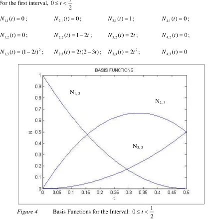
For the first interval,

2 1 0≤t <

0 ) (

1 , 1 t =

N ; N2,1(t)=0; N3,1(t)=1; N4,1(t)=0;

0 ) (

2 , 1 t =

N ; N2,2(t)=1−2t; N3,2(t)=2t; N4,2(t)=0;

2 3

,

1 (t) (1 2t)

N = − ; N_2,3(t)=2t(2−3t); 2 3

,

3 (t) 2t

N = ; N_4,3(t)=0

Figure 4 Basis Functions for the Interval:

2 1 0≤t <

The plots of the first interval basis functions, in Figure 4, show some different

characteristics from the plots with no intermediate points. Notice now that the second and

third functions end at the intermediate knot vector point value. N1, 3

N2, 3

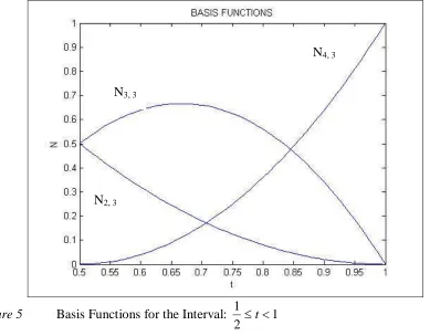
For the second interval, 1 2

1 < ≤t

0 ) (

1 , 1 t =

N ; N2,1(t)=0; N3,1(t)=0; N4,1(t)=1; N5,1(t)=0;

0 ) (

2 , 1 t =

N ; N2,2(t)=0; N3,2(t)=2−2t; N4,2(t)=2t−1; N5,2(t)=0;

0 ) (

3 , 1 t =

N ; N2,3(t)=2(t−1)2; ( ) 6 8 2 2

3 ,

3 t =− t + t−

N ; N4,3(t)=(1−2t)2; N5,3(t)=0

The plots of the second interval basis functions are shown in Figure 5. Notice now

that the second and third basis functions start at the intermediate knot vector point value and

end at a value of zero. Also notice that the first basis function is gone in this interval and a

fourth one was added. As was the case earlier for the last basis functions, its values start at

zero and end at one.

Figure 5 Basis Functions for the Interval: 1 2

1 _{≤ <}

t

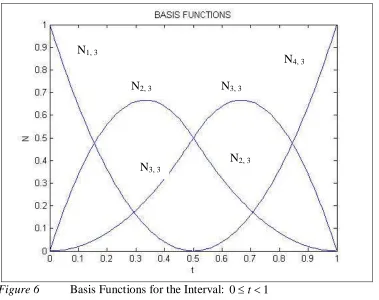
By combining the graphs of the two intervals, as seen in Figure 6, the main advantage

of using intermediate points in the knot vector can be seen. All of the second degree basis

functions join together at the interval line and form pseudo third degree basis functions. The N2, 3

N4, 3

joined together functions increase the overall accuracy, an advantage typical of a higher order

function, while not increasing the order of the basis functions.

Figure 6 Basis Functions for the Interval: 0≤t<1

Generally, the higher the order of the basis functions, the longer the computation time

associated with the problem. In addition to the increased time, the higher order also makes

the solution of under damped problems more susceptible to spurious oscillations. Therefore,

the addition of intermediate points in the knot vector can help by dividing the basis functions

into smaller piecewise segments. The smaller piecewise segments have the beneficial effect

of increasing the resolution of the approximation without increasing the order of the

functions.

2.2.3 Control Points

Once the knot vectors and basis functions have been determined, the last remaining

element needed to create the B-spline curve is the position vector, Bi. The coordinates that

make up these vectors are referred to as control points and they locate the vertices of the N1, 3

N2, 3 N3, 3

N4, 3

defining polygon. The control points are selected in order to yield an accurate approximation

to the desired curve.

The method used in this thesis to locate the abscissa control points is the Greville

Abscissa approach. If the abscissa values of the control points are restricted to lie at the

Greville Abscissa for the B-spline curve, the parametric coordinate ‘t’ is constrained to the

‘x’ Cartesian coordinate. The formula for calculating these coordinates is:

) ...

( 1

1

1 + −

+ + +

+

= i i i n

i t t t

n

x For i=0, 1,…,g-n (4)

where ‘n’ is the degree of the basis functions, or k – 1 and ‘g’ is the total number of knots in

the knot vector.

Example: [0 0 0 1 1 1] k = 3; n = 2; m = 6

0 ) 0 0 ( 2 1 ) ( 2 1

1 0

0 = t +t = + =

x

0 ) 0 0 ( 2 1 ) ( 2 1

2 1

1 = t +t = + =

x

2 1 ) 1 0 ( 2 1 ) ( 2 1

3 2

2 = t +t = + =

x

1 ) 1 1 ( 2 1 ) ( 2 1

4 3

3 = t +t = + =

x

1 ) 1 1 ( 2 1 ) ( 2 1

5 4

4 = t +t = + =

x

If calculated properly, there will always be two repeating values at the ends, one of which

can be dropped for the purposes of the B-spline curve derivation. In this example, x and ₀

4

2.3

Derivatives

Once the computation of the knot vectors, basis functions and control points is

completed, the B-spline curves can be calculated. Since computing the B-spline curve to

approximate the solution of a boundary value problem is the goal of this technique,

calculating the derivatives of the B-spline curve is necessary. The equations for the first two

derivatives, with respect to the parameter ‘t’ are:

∑

=

= 1

1 '

, ( ) )

( '

n

i

k i iN t

B t

P (5)

∑

=

= 1

1 '' , ( ) )

( ' '

n

i

k i iN t

B t

P (6)

Also notice once again, that the basis functions that are used are only the ones that represent

the highest order, k. When using B-spline curves and their derivatives to approximate the

solution to Boundary Value Problems, typically the boundary conditions are with respect to

Cartesian coordinates. Since the B-spline curves are functions of the parametric coordinate

system and B-spline derivatives are with respect to parametric coordinates, they must be

converted to the Cartesian coordinate system. In addition, the normalizing of the knot vector

done earlier must also be accounted for. For the first order, the derivative of the basis

function with respect to ‘x’ is:

x t N_ik

∂ ∂ _, ( )

    ∂ ∂ ∂

∂ =

x t t

t N_ik

* ) ( ,

(7)

It was stated earlier that when the Greville Abscissa are used to compute the control points

the Cartesian coordinate ‘x’ is constrained to the parametric coordinate ‘t’. That is, x = h * t,

or

    =     ∂ ∂

h x

t 1

into equation (7), the expression for the first derivative of the basis function with respect to

the Cartesian coordinate system becomes:

    ∂ ∂ = ∂ ∂ = • h t t N x N

N_i,k i,k i,k( )* 1 (8)

Consequently the first derivative of the B-spline function with respect to the Cartesian

coordinate system then becomes:

    =

∑

Similarly, the second derivative of the basis function can be shown to be:

2 2 , 2 , 1 ) (               ∂ ∂ = • • h t t N

N_ik ik (10)

The second derivative of the B-spline function with respect to the Cartesian coordinate

system then becomes:

2 1 1 '' , 1 ) ( ) (     =

∑

In general, it can be shown that:

a a k i a a k i h t t N N               ∂ ∂

= , ( ) 1 ) ( , (12) a n i a k i i h t N B t P     =

∑

N is the ‘a’th derivative with respect to Cartesian coordinate‘x’ and N, (t)

a k

i is the

3

One Dimensional B-spline Collocation

The B-spline collocation method involves the determination of knot vectors and

control points such that the differential equation, or boundary value problem, is satisfied to

some tolerance at a finite set of collocation points. These collocation points reside on the

Cartesian abscissa axis. The selection of these points appears to be arbitrary [18] and

throughout the literature there are many different ways used to select these collocation points.

As discussed previously, the four main types of spline collocation are the Nodal, Orthogonal,

Extrapolated/Modified and Collocation-Galerkin approaches. There have been many

variations of these four types used in the literature to solve mathematical models.

For this thesis, a variation on the Nodal type, called the Greville Abscissa approach

[18-19], has been selected and the collocation points are located at the Greville Abscissa

points along the Cartesian abscissa axis. Since these points have already been calculated and

the selection of the collocation points is arbitrary, the Greville Abscissa points are a logical

selection for the collocation points. Additional benefits of using this approach were

previously discussed when calculating the derivatives of the B-spline curves.

Once the collocation method has been selected, the one dimensional B-spline

collocation method to approximate a differential equation or boundary value problem

solution involves following a few steps.

1. Select the appropriate knot vector

2. Calculate all required basis functions, using equation (2) and (3)

3. Calculate abscissa coordinates for the required control points, using the Greville Abscissa

equation (4)

5. If necessary, use the boundary conditions to solve for end ordinate values of control

points

6. Substitute B-spline curves and the derivatives into differential equation or boundary

value problem

7. Calculate the remaining interior ordinate coordinates of the control points by evaluation

of the differential equation at the corresponding abscissa of the collocation points

In order to quantify the approximation results, the error has been calculated at each

collocation point using the relative error formula:

100 * 1

% _

  

 

− =

Exact BSpline

ERR (14)

A statistical sampling method has been employed in order to quantify a baseline value for the

overall approximation procedure. The statistical method chosen for use is the Root Mean

Squares method. This technique is used throughout industry for tolerance analysis. The

formula for the Root Mean Squares method is:

(

)

∑

= N

i ERR i

N RMS

1

2 % *

1

(15)

A baseline value for a successful approximation has been set at RMS < 0.5% for the entirety

of this research. One of the objectives of this research is to compare the speed and accuracy

of the B-spline Collocation Method with two different techniques. The first is by increasing

the number of internal points in the knot vector and the second is by increasing the

approximation to a higher order. In order to accomplish this, the B-spline Collocation

Method solution is compared to analytical solutions that can be easily computed. If an

analytical situation is not available, selecting convergence criteria would be more applicable

when calculating the solution at the collocation points. To ensure an even higher level of

their values converge. The residuals are the solution errors at points in addition to the

collocation points. If an even higher level of accuracy is required, increase the density of the

evaluating points that are calculated.

Three types of one-dimensional problems were evaluated for this thesis in order to

calculate the effectiveness of the B-Spline Collocation Method. The approximations of both

over-damped and un-damped, second order boundary value problems, as well as, a fourth

order, Euler-Bernoulli beam problem have been evaluated. Please note that to get to the

solution of each problem, one must go through the same 7 steps mentioned previously.

3.1

Example 1A

Over Damped, Second Order ODE Approximated with a Third Order B-spline, with No Intermediate Knot Vector Points

P’’ + 2P’ + P = 0 For 0< x<1 Where P’ =

x

∂ ∂

Boundary Conditions: P(0) = 0, P(1) = 1

1. The first step in the B-spline collocation method is to select the appropriate knot vector

that provides the resolution required for the problem. A third order, open-uniform knot

vector has been selected.

[0 0 0 1 1 1]

2. The second step is to calculate all required basis functions using equations (2) and(3).

otherwise x t x t

N_i,1 i i 1

0 1 )

( ≤ < +

   =

1 1 , 1 1

1 , ,

) ( )

( ) ( ) ( ) (

+ +

− + +

− +

−

− − +

− − =

i k i

k i k i

i k i

k i i k

i

x x

t N t x x

x

t N x t t N

0 ) (

1 , 1 t =

N ; N_2,1(t)=0; N_3,1(t)=1; N_4,1(t)=0;

0 ) (

2 , 1 t =

N ; N2,2(t)=1−t; N3,2(t)=t; N4,2(t)=0;

2 3

,

1 (t) (1 t)

N = − ; N2,3(t)=2t(1−t);

2 3

, 3 (t) t

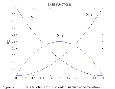
By plotting the k = 3 basis functions, the generated curves can be used to verify that the

calculated basis functions comply with the criteria discussed in the previous chapter. In

Figure 7, it can be seen that indeed they do meet the required criteria and it is safe to

move on to the next step.

Figure 7 Basis functions for third order B-spline approximation

3. The next step is to calculate the abscissa coordinates for the control points. Since the

Greville Abscissa approach has been chosen, use equation (4) to calculate the Greville

Abscissa for required control points.

) ...

( 1

1

1 + −

+ + +

+

= i i i n

i t t t

n

x For i=0, 1,…,m-n

0 ) 0 0 ( 2 1 ) ( 2 1

1 0

0 = t +t = + =

x

0 ) 0 0 ( 2 1 ) ( 2 1

2 1

1 = t +t = + =

x

N1, 3

N2, 3

2 1 ) 1 0 ( 2 1 ) ( 2 1 3 2

2 = t +t = + =

x 1 ) 1 1 ( 2 1 ) ( 2 1 4 3

3 = t +t = + =

x 1 ) 1 1 ( 2 1 ) ( 2 1 5 4

4 = t +t = + =

x

As discussed in the previous chapter, the repeating values of x₀ =0 and x₄ =1 should be

dropped. That leavesx₁ =0,

2 1

2 =

x and x₃ =1 as the abscissa coordinates for the

control points.

4. The fourth step is to calculate the appropriate B-spline curve equations and the required

derivatives for the boundary conditions that need to be met. Since the third term of the

differential equation and both boundary conditions involve the B-spline curve, it must be

calculated. The B-spline curve must be calculated, by using equation (1).

∑

B t P ) ( ) ( ) ( )

(t B1N1,3 t B2N2,3 t B3N3,3 t

P = + +

[

]

[

]

[ ]

3 2

2

1 (1 ) 2 (1 )

)

(t B t B t t B t

P = − + − +

Since the second term of the differential equation involves the first derivative, the first

derivative of the B-spline equation must be calculated, using equation (5).

∑

B t P ) ( ' ) ( ' ) ( ' ) (

' t B₁N_1,3 t B₂N _2,3 t B₃N _3,3 t

P = + +

[

]

[

]

[ ]

B t

P'( )= ₁ 2( −1) + ₂ (2−4 ) + ₃ 2

The first term of the differential equation involves the second derivative. The second

∑

=

= 1

1 '' , ( ) )

( ' '

n

i

k i iN t

B t

P

) ( '' )

( '' )

( '' )

(

'' t B₁N _1,3 t B₂N _2,3 t B₃N _3,3 t

P = + +

[ ]

[

]

[ ]

(

'' t B₁ B₂ B₃

P = + − +

5. The next step is to use the boundary conditions to solve for end ordinate values of control

points. Since the Greville Abscissa were used as control points, the parametric coordinate

‘t’ is constrained to the Cartesian coordinate ’x’ and it becomes a direct substitution. The

boundary conditions were P(0) = 0 and P(1) = 1. When the B-spline curve,

[

]

[

]

[ ]

3 2

2

1 (1 ) 2 (1 )

)

(t B t B t t B t

P = − + − + , is evaluated at the boundaries, the following

external ordinate values are calculated to be:

P(0) = 0B1 = 0y1 =0

P(1) = 1 B3 = 1y3 =1

6. The sixth step is to substitute B-spline curve and the derivatives into the differential

equation, P’’ + 2P’ + P = 0, we get

[ ]

[

]

[ ]

{

}

{

[

]

[

]

[ ]

}

{

[

]

[

]

[ ]

}

Now using the ordinate values from the previous step, the differential equation reduces

to:

{

[

] [ ]

}

{

[

] [ ]

}

{

[

]

[ ]

}

2 2

2 − + + B − t + t + B t −t +t =

B

7. The seventh step is to calculate the remaining internal ordinate coordinates of the control

points by evaluation of the previously reduced differential equation,

[

] [ ]

{

}

{

[

] [ ]

}

{

[

]

[ ]

}

coordinates. At‘t’ = ½, the remaining internal ordinate coordinate is calculated to be:

Now that all of the coordinates for the control points have been calculated, they can be

substituted into the B-spline curve equation,

[

]

[

]

[ ]

2

1 (1 ) 2 (1 )

)

(t B t B t t B t

P = − + − + to give

the final equation for the B-spline approximation. Since the B-spline curve is in terms of the

parametric coordinate system and the desired result is an equation in the Cartesian coordinate

system, a bit of manipulation is required. As stated earlier, using the Greville Abscissa allows

a direct substitution of the ‘x’ and‘t’ parameters. The B-spline function approximation

equation then becomesP(x)=0.82353

[

]

[ ]

Now a comparison of the B-spline function approximation and the exact solution,

P(x) = 2.718*x*e−x, must be done to determine the accuracy of the collocation method. The first step to determining the accuracy is to evaluate both the B-spline function approximation

and the exact solution at the collocation points. Next, calculate the relative error percentage,

by using equation (14) for each collocation point. These values have been listed in Table 1.

Point Approximate Exact %Error

0 0 0 0

0.5 0.85714 0.82428 3.99

1 1 0.9999 0.001

Collocation Point Evaluation

Table 1 Table of collocation points for Example 1a

Once all of the relative error percentage calculations have been done, the Root Mean Squared

Error must be computed, by using equation (15).

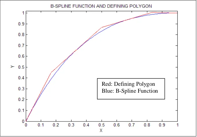
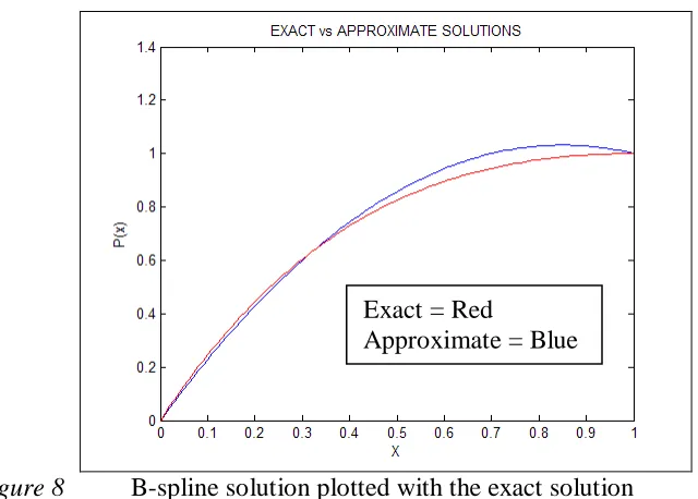
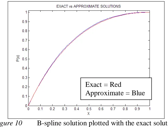
Figure 8 B-spline solution plotted with the exact solution

The RMS Error of 2.3% is greater than the 0.5% baseline, previously established. By

plotting the two functions for the entire range, as seen in Figure 8, the areas where refinement

is necessary can be determined. One method of refinement is to increase the order of the

B-spline Basis Functions. Another method is to add a collocation point within the range where

the highest error percentage is. By a visual inspection of Figure 8, it can be seen that the

largest difference between the two functions is within the range of 0.6 < x < 0.8. The next

example (1b) shows what will happen when two additional collocation points are added. In

order to add two collocation points, two intermediate points are added to the knot vector.

3.2

Example 1B

Over Damped, Second Order ODE Approximated with a Third Order B-spline, with Two Intermediate Knot Vector Points

P’’ + 2P’ + P = 0 For 0< x<1

Boundary Conditions: P(0) = 0, P(1) = 1

1. Once again, the first step is to select the appropriate knot vector. A third order,

open-uniform knot vector with two intermediate points has been selected.

[0 0 0 1/3 2/3 1 1 1]

Exact = Red

2. The next step is to calculate all of the required basis functions for each range of values of

the parameter ’t’ using equations (2) and (3).

otherwise x t x t

N_i,1 i i 1

0 1 )

( ≤ < +

   = 1 1 , 1 1 1 , , ) ( ) ( ) ( ) ( ) ( + + − + + − + − − − + − − = i k i k i k i i k i k i i k i x x t N t x x x t N x t t N 3 1 0≤t<

0 ) (

1 , 1 t =

N ; N2,1(t)=0; N3,1(t)=1; N4,1(t)=0;

0 ) (

2 , 1 t =

N ; N_2,2(t)=1−3t; N_3,2(t)=3t; N_4,2(t)=0;

2 3

,

1 (t) (1 3t)

N = − ; (4 9 )

2 3 ) ( 3 , 2 t t t

N = − ;

2 9 ) ( 2 3 , 3 t t

N = ; N4,3(t)=0

3 2 3 1 < ≤t 0 ) ( 1 , 2 t =

N ; N3,1(t)=0; N4,1(t)=1; N5,1(t)=0;

0 ) (

2 , 2 t =

N ; N3,2(t)=2−3t; N4,2(t)=3t−1; N5,2(t)=0;

2 ) 3 2 ( ) ( 2 3 , 2 t t

N = − ; (6 6 1)

2 3 ) ( 2 3 ,

3 − +

−

= t t

t N ; 2 ) 3 1 ( ) ( 2 3 , 4 t t

N = − ; N5,3(t)=0

1 3 2 < ≤t 0 ) ( 1 , 2 t =

N ; N3,1(t)=0; N4,1(t)=0; N5,1(t)=1;

0 ) (

2 , 2 t =

N ; N3,2(t)=0; N4,2(t)=3−3t; N5,2(t)=3t−2;

0 ) (

3 , 2 t =

N ; 2 ) 1 ( 9 ) ( 2 3 , 3 − = t t

N ; (9 14 5)

2 3 ) ( 2 3 ,

4 − +

−

= t t

t

N ; 2

3 ,

5 (t) (2 3t)

N = −

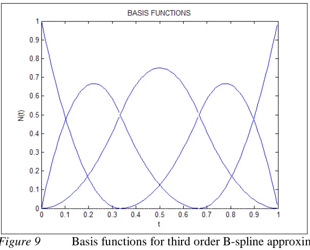
By plotting the k = 3 basis functions for each interval together, as shown in Figure 9, it can

Figure 9 Basis functions for third order B-spline approximation with two intermediate Knot Vector points

3. The third step is to calculate all of the abscissa coordinates values for the required control

points, using the Greville Abscissa formula, equation (4).

) ...

( 1

1

1 + −

+ + +

+

= _{i i i n}

i t t t

n

x For i=0, 1,…,m-n

0 ) 0 0 ( 2 1 ) ( 2 1 1 0

0 = t +t = + =

x 0 ) 0 0 ( 2 1 ) ( 2 1 2 1

1 = t +t = + =

x 6 1 ) 3 1 0 ( 2 1 ) ( 2 1 3 2

2 = t +t = + =

x 2 1 ) 3 2 3 1 ( 2 1 ) ( 2 1 4 3

3 = t +t = + =

x 6 5 ) 1 3 2 ( 2 1 ) ( 2 1 5 4

4 = t +t = + =

x 1 ) 1 1 ( 2 1 ) ( 2 1 6 5

5 = t +t = + =

x 1 ) 1 1 ( 2 1 ) ( 2 1 7 6

6 = t +t = + =

Once again, the two repeating values at the ends should be dropped and that will

leavex₁ =0,

6 1 2 = x , 2 1 3 = x , 6 5 4 =

x and x5 =1 as the abscissa coordinates for the

control points.

4. The fourth step is to calculate the appropriate B-spline curve equations and the required

derivatives for the boundary conditions that need to be met. Since the third term of the

differential equation and both boundary conditions involve the B-spline curve, it must be

calculated for each range of the parameter‘t’. The B-spline curve must be calculated, by

using equation (1).

For

3 1

0≤t <

∑

+ = = 1 1 , ( ) ) ( n i k i iN t

B t P ) ( ) ( ) ( )

(t B₁N_1,3 t B₂N_2,3 t B₃N_3,3 t

P = + +

[

]

≤t

∑

+ = = 1 1 , ( ) ) ( n i k i iN t

B t P ) ( ) ( ) ( )

(t B2N2,3 t B3N3,3 t B4N4,3 t

P = + +

      − +    − _{− +} +       − = 2 ) 3 1 ( ) 1 6 6 ( 2 3 2 ) 3 2 ( ) ( 2 4 2 3 2 2 t B t t B t B t P

For 1

3 2

<

≤t

∑

+ = = 1 1 , ( ) ) ( n i k i iN t

B t P ) ( ) ( ) ( )

(t B₃N_3,3 t B₄N_4,3 t B₅N_5,3 t

P = + +

[

]

5 2

4 2

3 (9 14 5) (2 3)

2 3 2 ) 1 ( 9 )

(t B t B t t B t

P _+ _− − + _+ −

Since the second term of the differential equation involves the first derivative, the first

derivative of the B-spline equation must be calculated for each range of the parameter‘t’,

using equation (5).

For

3 1

0≤t <

∑

+ = = 1 1 ' , ( ) ) ( ' n i k i iN t

B t P ) ( ' ) ( ' ) ( ' ) (

' t B1N1,3 t B2N 2,3 t B3N 3,3 t

P = + +

[

]

[

]

[ ]

t

P'( )= 118 −6 + 2 6−27 + 3 9

For 3 2 3 1 <

≤t

∑

+ = = 1 1 ' , ( ) ) ( ' n i k i iN t

B t P ) ( ' ) ( ' ) ( ' ) (

' t B2N 2,3 t B3N 3,3 t B4N 4,3 t

P = + +

[

]

[

]

[

]

) (

' t =B2 t− +B3 − t +B4 t−

P

For 1

3 2

<

≤t

∑

+ = = 1 1 ' , ( ) ) ( ' n i k i iN t

B t P ) ( ' ) ( ' ) ( ' ) (

' t B3N 3,3 t B4N 4,3 t B5N 5,3 t

P = + +

[

]

[

]

[

]

) (

' t =B₃ t− +B₄ − t +B₅ t−

P

The first term of the differential equation involves the second derivative. The second

derivative of the B-spline curve can be calculated for each range of the parameter‘t’, using

equation (6).

For

3 1

0≤t <

∑

+ = = 1 1 '' , ( ) ) ( ' ' n i k i iN t

B t P ) ( '' ) ( '' ) ( '' ) (

'' t B₁N _1,3 t B₂N _2,3 t B₃N _3,3 t

P = + +

[ ]

[

]

[ ]

(

'' t B₁ B₂ B₃

For 3 2 3 1 <

≤t

∑

+ = = 1 1 '' , ( ) ) ( ' ' n i k i iN t

B t P ) ( '' ) ( '' ) ( ' ' ) (

'' t B₂N _2,3 t B₃N _3,3 t B₄N _4,3 t

P = + +

[ ]

[

]

[ ]

(

'' t B₂ B₃ B₄

P = + − +

For 1

3 2 _{≤ <}

t

∑

+ = = 1 1 '' , ( ) ) ( ' ' n i k i iN t

B t P ) ( ' ' ) ( ' ' ) ( '' ) (

'' t B3N 3,3 t B4N 4,3 t B5N 5,3 t

P = + +

[ ]

[

]

[ ]

(

'' t B₃ B₄ B₅

P = + − +

5. The next step is to use the boundary conditions to solve for end ordinate values of control

points. Since the Greville Abscissa were used as control points, the parametric coordinate

‘t’ is constrained to the Cartesian coordinate ’x’ and it becomes a direct substitution. The

boundary conditions were P(0) = 0 and P(1) = 1. Since the B-spline curve is a function

over multiple ranges, the appropriate range must be used when calculating the external

ordinate values.

For

3 1

0≤t <

[

]

     +     ₋ + − = 2 9 ) 9 4 ( 2 3 ) 3 1 ( ) ( 2 3 2 2 1 t B t t B t B t P

P(0) = 0B1 = 0y1 =0

For 1

3 2

<

≤t ₄ 2 ₅

[

]

2

3 (9 14 5) (2 3 )

2 3 2 ) 1 ( 9 )

(t B t B t t B t

P + −

   − _{− +} +       − =

P(1) = 1B5 = 1y5 =1

6. The sixth step is to substitute B-spline curves and the derivatives into original differential

For

3 1 0≤t <

[ ]

[

]

[ ]

{

}

{

[

]

[

]

[ ]

}

[

]

2 9 ) 9 4 ( 2 3 ) 3 1 ( 2 3 2 2 1 =             +     ₋ +

− t B t t B t

B

Now using the ordinate values from the previous step, the differential equation for this range

reduces to:

[

]

[ ]

{

}

{

[

]

[ ]

}

2 9 ) 9 4 ( 2 3 9 27 6 2 9 ) 27 ( 2 3 2 3 2 3 2 =             +     ₋ + + − + +

− B B t B t B t t B t

B For 3 2 3 1 < ≤t

[ ]

[

]

[ ]

{

}

{

[

]

[

]

[

]

}

0 2 ) 3 1 ( ) 1 6 6 ( 2 3 2 ) 3 2 ( 2 4 2 3 2 2 =             − +    − _{− +} +     

 − t

B t t B t B

For 1

3 2

< ≤t

[ ]

[

]

[ ]

{

}

{

[

]

[

]

[

]

}

[

]

Once again using the ordinate values from the previous step, the differential equation for this

range reduces to:

[ ]

[

] [ ]

{

}

{

[

]

[

] [

]

}

[

]

9 2 2

7. The seventh step is to calculate the remaining internal ordinate coordinates of the control

points by evaluation of the previously reduced differential equation, using the appropriate

range. At ‘t’ = 0.1667, using the equation for the range

3 1 0≤t< ,

[

]

[ ]

{

}

{

[

]

[ ]

}

2 9 ) 9 4 ( 2 3 9 27 6 2 9 ) 27 ( 2 3 2 3 2 3 2 =             +     ₋ + + − + +

− B B t