A multidirectional Physarum solver for the automated design of space trajectories

A Multidirectional Physarum Solver for the

Automated Design of Space Trajectories

Luca Masi

Mechanical & Aerospace Department University of Strathclyde

Glasgow, UK, G11XJ Email: [email protected]

Massimiliano Vasile

University of Strathclyde Glasgow, UK, G11XJ

Email: [email protected]

Abstract—This paper proposes a bio-inspired algorithm to automatically generate optimal multi-gravity assist trajec-tories. The multi-gravity assist problem has some analogies with the better known Traveling Salesman Problem and can be addressed with similar strategies. An algorithm drawing inspiration from the Physarum slime mould is proposed to grow and explore a tree of decisions that corresponds to the possible sequences of transfers from one planet to another. Some examples show that the proposed bio-inspired algorithm can produce solutions that are better than the ones generated by humans or with Hidden Genes Genetic Algorithms.

I. INTRODUCTION

A gravity assist manoeuvre exploits the gravity of a planet to change the velocity of a spacecraft. As a result, sub-stantial modifications of the orbital motion of the spacecraft can be obtained without the use of its propulsion system. An optimal sequence of gravity assist maneuvers can make chal-lenging targets, like Saturn, accessible. The effectiveness of a sequence of gravity assist maneuvers depends on the choice of the planets (called swing-by planets in the following) and of the timing of the encounters with each planet. The problem of finding the sequence of planets and encounter dates (including resonances, or multiple encounters with the same planet) that provides the best transfer to a target object is a challenging combinatorial problem, referred to as the MGA problem, or MGAP, in this paper.

Deterministic algorithms for the solution of the MGAP are based on simplified models and an enumerative search like PAMSIT [1], or a two stage approach in which a list of possible sequences is derived from an analysis of the Tisserand’s graph or from simple energetic considerations [2] and a search for optimal dates is then performed with a branch and prune type of procedure for each of the sequences.

Bio-inspired techniques for the solution of the MGAP can be found in [3], [6], [5]. In [3] the authors proposed a hybrid branch & prune and evolutionary process that could automatically generate sequence and optimal multi-gravity assist transfer with Deep Space Maneuvers (DSM’s) in a single loop. In [6] and [5] the problem is approached by using Hidden Genes Genetic Algorithms (HGGA) where each sequence is represented by a binary chromosome. The generation of an optimal solution goes through two loops:

an outer loop and an inner loop. The outer loop generates the sequence of planets through a Hidden Genes Genetic Algorithm. The inner loop takes the sequence generated by the outer loop and computes an optimal set of encounter dates. Previous work by Ceriotti and Vasile [4] showed the potentiality of Ant Colony Systems at effectively solving the MGAP. The MGAP is translated into a planning and scheduling problem in which a solution is incrementally built with a modified Ant Colony Optimization algorithm.

The bio-inspired heuristic presented in this paper takes inspiration from the behaviour of a simple amoeboid or-ganism, the Physarum Polycephalum, that is endowed by nature with simple heuristics that can solve complex discrete decision making problems. For example, it was shown that the Physarum Polycephalum is able to find the shortest path through a maze [9], recreate the Japan rail network, reproduce the designed highway network among several Mexican cities [7], solve multi-source problems with a simple geometry [8], [10], mazes [11] and transport network problems [11].

The algorithm presented in this paper is first applied to the solution of the classic Traveling Salesman Problem (TSP), and then to two instances of the MGA problem: a simple energy-based two dimensional problem without con-sidering the actual ephemerides of the planets, and a more complex three dimensional problem with real ephemerides.

II. MULTI-DIRECTIONALDISCRETEDECISION

MAKING

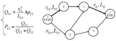
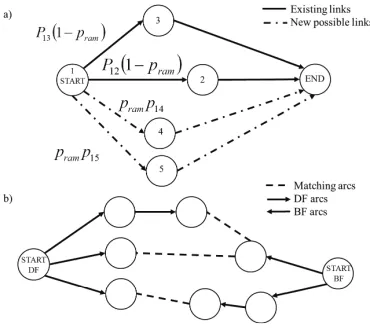
Fig. 1. Figure showing a simple graph: thicker arrows represent higher fluxes. In this exampleQ12> Q13⇒P12> P13.

Fig. 2. Figure showing ramification towards a new node (a) and matching between decision paths in DF and BF (b).

multiple directions. They are presented in this section along with a restart procedure that mitigates the risk of stagnation. The pseudocode of the multidirectional incremental modified Physarum solver is provided in Algorithm 1.

1) Decision network exploration: The flux through the net ofPhysarumveins can be modelled as a classical Hagen-Poiseuille flow in cylindrical ducts with diameter variable with time [8], [10], [11]:

Qij =πr

4

ij 8µ

∆pij

Lij (1)

where Qij is the flux between i and j, µ is the dynamic viscosity,rijthe radius,Lij the length and∆pijthe pressure gradient. These quantities are shown in the simple graph in Fig. 1. A variation in the diameter of the veins allows for a change in the flux. The dilation of the veins due to an increase in the flowing nutrients can be modelled using a monotonic function of the flux:

d dtrij

dilation

=f(Qij) (2)

where f(0) = 0 , i.e., linear, sigmoidal, etc. It can be assumed that the dynamics of the veins is sufficiently slow for the flow to be considered in steady state [10] regime. The contraction of the veins, due to evaporative effects, can be assumed to be directly proportional to their radius:

d dtrij

contraction

=−ρrij (3)

whereρ∈[0,1]is a pre-defined evaporation coefficient.

The probability associated with each vein connectingi andjis then computed using a simple adjacency probability matrix based on fluxes:

Pij=

{ _Q

ij

∑

j∈NiQij if j∈Ni

0 if j /∈Ni (4)

whereNi is the set of neighbouring veins to a node i.

TABLE I. SETTING PARAMETERS FOR THE MODIFIEDPHYSARUM SOLVER

m Linear dilation coefficient, see Eq. (6). ρ Evaporation coefficient, see Eq. (3). GF Growth factor, see Eq. (5) Nagents Number of virtual agents.

pram Probability of ramification, see Sec. II.

λ Weight on ramification, see Eq. (8).

Algorithm 1Multidirectional Incremental Physarum Solver

1: initializem,ρ,GF,Nagents,pram,λ 2: foreach generationdo

3: foreach virtual agent in all directions (DF andBF) do

4: ifcurrent node̸=end nodethen 5: ifν ∈ U(0,1)≤pram then

6: using Eq. (8) create a new decision path,

building missing links and nodes

7: else

8: move on existing graph using Eq. (4).

9: end if 10: end if 11: end for

12: look for possible matchings, see Sec. II. 13: contract and dilate veins using Eqs. (2), (3), (5) 14: ifrij exceeds upper radius limit, see Eq. (7) then 15: block radius increment

16: end if

17: update fluxes and probabilities using Eqs. (1), (4) 18: ifrestart conditionthen

19: update veins’ radii using Eq. (9)

20: update fluxes and probabilities using Eqs. (1), (4) 21: end if

22: end for

A further term in the dilation process was added in the algorithm and takes inspiration from the behaviour of the amoeba Dictyostelium discoideum. In its aggregative and slug stages, amoebae are chemotactically sensitive to a chemical known as cyclic Adenosine Monophosphate (cAMP). A starving pacemaker amoeba starts to emit cAMP, that is a call for aggregation and subsequent collective behaviour. In a computational algorithm, pacemaker can be considered the agent with best objective function. A linear dilation for the pacemaker, which is defined as the best path so far in the decision graph in terms of objective function, was here chosen:

d dtrijbest

elasticity

=GF rij_best (5)

where GF is the growth factor of the best chain of veins and rijbest the veins’ radii. This pacemaker call can be

interpreted as a variable elasticity of the veins with time: best veins increase their capacity of dilation with a percentage GF. This is an additive term in the veins’ dilation process, whose first main term is expressed in Eq. (2).

flux in each vein is proportional to the fourth power of the radius and inversely proportional to the length. Once a vein is selected by a virtual agent in a generation, its radius is incremented using Eq. (2). In the present work, a function linear with respect to the product between the radiusr_ij(k)of the veins traversed by agentk, and the inverse of the total cost of the decision taken by agent k, i.e., the total length L(_totk), will be used for the veins’ dilation:

d dtr

(k)

ij

dilation

=mr

(k)

ij

L(totk)

(6)

where the coefficient m is here called linear dilation coef-ficient. Evaporation is taken into account using Eq. (3) for each agent. Fluxes are then calculated using Eq. (1) and probabilities are updated in accordance with Eq. (4). This mechanism of veins’ diameter and flux updating corresponds to line 13 of Algorithm 1, where Eq. (5) contributes to the veins’ growth of the pacemaker. An upper limit on the maximum vein radius was introduced in order to avoid veins’ flux explosion and limit the converge rate. If the radiusrij exceeds a maximum valuermax, the vein dilation is stopped until the radius returns again below rmax for the effect of evaporation. This upper limit, calledkexplosion, is given as the ratio betweenrij andrini:

kexplosion= rij

rini (7)

whereriniis the initial radius of the veins. This mechanism corresponds to lines 14 to 16 of Algorithm 1.

2) Unidirectional Growth of the Decision Network: The incremental growth of the decision network in one direction is performed in parallel by a set of virtual agents. At every node of the tree, each agent either generates a new branch or moves along an existing one. At each node, the agent has a probability pram of ramification towards new nodes that are not yet linked with the current one. On line 5 of Algorithm 1, a random numberν is drawn from a uniform distributionU(0,1)and the conditionν < pram is verified. Assuming that the agent is at nodei, if ramification is the choice, the agent evaluates the set of possible new branches and assigns a probabilitypij of constructing a new link from the current nodeito a new possible nodej∈Ni, where¯ Ni¯ is the set of unlinked nodes (for example nodes 4 and 5 in Fig.2(a)), according to:

pij∝ 1

Lλ ij

(8)

whereλis a pre-defined exponent. Fig. 2(a) shows a possible ramification from the start node: dotted lines represent feasible branches not yet existing. If an agent is at the start node it has a probability pram of ramification towards the unlinked nodes 4 and 5. If the agent decides to create a new link, a new node is selected according to Eq. (8), see line 6 of Algorithm 1.

If a set of linked nodes is available, the agent can decide, with probability1−pram, to traverse the existing branches in the neighborhoodNi (see line 8 of Algorithm 1). In the case shown in Fig. 2(a) when an agent is at the start node, it can explore the already linked nodes 2 and 3. Once at node 2 or 3 the only possibility in order to complete the decision

path is a new link construction between the current node and ending node.

3) Multidirectional Growth of the Decision Network:

If multiple Physarum are simultaneously grown, one can explore the decision space from multiple directions. Here a bi-directional approach is presented in which twoPhysarum, calledDFandBF, form a network made of two superposed graphs. While growing, the two expanding Physarumhave the possibility of matching decision sequences: agents can build and traverse arcs that connect nodes belonging to

DF and BF Physarum respectively forming a single path from the heart of one Physarum to the heart of the other

Physarum, see line 12 of Algorithm 1.

Figure 2(b) shows a simple case of matching between the graphs associated to two amoebae. The matched decision path is given by the union of a route in the DF and one in the BF through a matching arc. Several types of matching strategies were implemented and tested. The most promising strategy proceeds as follows: the bestnseqBF and DF partial routes are taken and each DF route communicates with each of the BF routes. The communication process randomly selects a pair of nodes along the two routes and tries to connect the two nodes with a matching arc.

In the following, the top 10 routes generated in DF and BF are matched assuming an equal probability of cutting any of the arcs.

4) Restart Procedure: A restart procedure was added to mitigate the risk of stagnation at local minima. If a certain condition, here calledrestart condition, is reached, the veins’ radii are reset to:

rij =rini (9)

The restart procedure is based on the number of nodes and arcs in common between two decision sequences: after comparing all decision sequences among each other, if the

minimum number of nodes in common ncom

min exceeds a threshold nshare, the algorithm is restarted. The restart procedure is summarised at lines 18 to 21 of Algorithm 1.

The main parameters of the modified Physarum solver are summarized in Table I. The initial radius of the veins rini is always set equal to 1 in the simulations presented in this paper. The complete pseudocode of the multidirectional incremental modifiedPhysarumsolver is provided in Algo-rithm 1. The unidirectional algoAlgo-rithm is a special case of the multidirectional algorithm, obtained by freezing theBF, i.e., flux and graph growth are allowed in only one direction.

III. APPLICATION TO THETSP

The TSP, a classical problem in combinatorial optimiza-tion, was used as benchmark for the performance eval-uation of the modified unidirectional and multidirectional

Physarum algorithms. Given a set Ncities cities whose reciprocal distance l is known, the TSP is the problem of finding the shortest tour that visits each city exactly once. TSPLIB [16] was used to benchmark the proposedPhysarum

0 0.5 1 1.5 2 2.5 3 3.5 x 107 0

0.1 0.2 0.3 0.4 0.5 0.6 0.7 0.8 0.9

Success Rate

Function evaluations D

D&B

Fig. 3. Variation of the success rate with the number of function evaluations - Eil51 TSP test case.

m= 5×10−3_{,ρ= 10}−4_{,GF = 5×10}−3_,N

agents= 100, pram = 1, λ = 0. The value kexplosion = 5, see Eq. (7) and restart with nshare = dim₂ were selected, where dim is the number of cities. Fig. 3 reports the success rate (i.e., more runs successfully converge to the known best solution) over 200 independent runs and show that the multidirectional modifiedPhysarumalgorithm with matching ability (D&B) provides higher success rate than the unidirectional modified

Physarum algorithm (D) when applied to TSP problems. In particular for Eil51 the gain using D&B instead of D reaches approximately 20% at3×107 function evaluations. It should be noted that there is an initial transient phase where the performance of the multidirectional solver do not exceed the performance of the unidirectional solver because the two expandingPhysarumcause an initial increase in the number of function evaluations while the growth of the veins is still low. After this initial transient, the twoPhysarumstart to reduce the search space and the role of communication becomes crucial.

A. Comparison with Other Algorithms

Although the idea of this paper is to show that mul-tidirectionality increases the performance of the Physarum

algorithm, a comparison with known and tested algorithms is proposed in the following. Note that thePhysarumalgorithm does not contain either tailored heuristics for TSP or local optimization heuristics, like2-opt[18], or static or dynamic candidate lists [15], [14]. For this comparative test the Physarum was applied to the solution of problems Eil51,

Eil76,Eil101,Kroa100 andRat195of the TSBLIB.

1) ACS, MMAS, KniesG, KniesL, SA for TSP.: For this set of comparative tests, mean, best and standard deviation are used as performance indicators, see Table II and Ta-ble III, in order to have a fair comparison with the results in the literature. Values in Table II for the ACO-inspired algorithms are from [14], [15]. ACS is an implementation of Ant Colony System, while MMAS is a Max-Min Ant System algorithm, which is considered the state of the art of ACO-inspired algorithms. Table II shows that the proposed

Physarumalgorithm is comparable to state of the art ACS algorithms. The values in Table III are from [17]. KniesG refers to Kohonen Network Incorporating Explicit Statistics Global [12], KniesL to its local version [12], while SA

TABLE II. TSPBENCHMARK USED IN[14]WITH MEAN VALUE, STANDARD DEVIATION AND BEST VALUE AT3×107_{FUNCTION CALLS)}

Physarum MMAS ACS D&B

Eil51

mean 426.8 427.2 428.1 variance 0.92 1.13 2.48

best 426 426 426

Kroa100

mean 21352.9 21352.1 21420.0 variance 94.7 50.3 141.7 best 21282 21282 21282

ACS is from [14], 15 runs performed. MMAS is from [15], 25 runs performed. Physarum, 25 runs performed for Kroa100, 200 for Eil51.

TABLE III. TSPBENCHMARK FROM[17],MEAN VALUE AT107 FUNCTION CALLS

Physarum KniesG KniesL SA D&B

Eil51 427.8 438.2 438.2 435.9

Eil76 543.7 567.5 564.8 567.8

Eil101 649.8 664.4 658.3 665.1

Rat195 2397.0 2599.9 26073.0 2631.7

KniesG, KniesL, SA are from [17], runs performed n/a. Physarum, 200 runs performed.

indicates Simulated Annealing [13]. The results in this table demonstrate the superior ability of the Physarumalgorithm at finding good solutions for the test cases Eil51, Eil76,

Eil101 andRat195.

IV. MGAP 2D ENERGYMODEL

The MGAP is here formulated as a simple planar tra-jectory model. The motion of planets and the spacecraft is assumed to occur in a plane. The orbits of all the planets are assumed to be circular. The swing-by of a planet is assumed to produce an instantaneous variation of the velocity of the spacecraft with respect to the Sun. The variation of the velocity is only due to the gravity of the planet and no propelled maneuvers are considered in this model (see [1] for more details).

Given a sequence of planetary encounters{A, B, ...}, the modulus v_∞,L and the directionβ of the velocity vector of the spacecraft with respect to the velocity Vp of planet A at departure, the spacecraft follows an orbit with, at most, two intersections with the orbit of the following planet in the sequence (see Fig. 4). With reference to Fig. 4, if Planet A is the Earth and the launch happens at 4, then, if no resonances are considered, at most two possible transfer arcs are possible: 4-1 and 4-2. This is true for each transfer between two planets. Note that planets are assumed to always be at the intersection points thus no actual phasing is considered.

Fig. 4. Initial conditions and different transfers on the same orbit.

TABLE IV. SUCCESS RATE: PHYSARUM, PHYSARUMD&B. EARTH TOJUPITER TRANSFERS: EJ7 (v_∞,L= 7km/s,α= 1.5π), EJ5

(v_∞,L= 5km/s,α= 1.5π)

Success Rate

Instance EJ5 EJ7

Func. eval. 5000 , 30000 5000 , 30000

Physarum 0.66 0.80 0.16 0.81 Physarum D&B 0.45 0.93 0.55 0.94

Relative Simulation Time

Instance EJ5 EJ7

Func. eval. 30000 30000

Physarum 1 1

Physarum D&B 0.74 0.68

in Fig. 2. For the solution of this particular instance of the MGAP, the decision tree is built only forward while it is explored both forward and backward. The matching process links complete paths explored backwards to partial paths generated and explored forward.

The cost of each transfer from intersection i to inter-section j is the time of flightT oFij and the total objective function, to be minimised, is the total time of flightT oFtot. The Physarum algorithm is applied by replacing L(_totk) in Eq. (1) and Lij in Eq. (6) respectively with T oF_tot(k) and T oFij. The length of the sequence of planets is bounded from above with an upper limit of 4 consecutive swing-by’s.

The Physarum and the Multidirectional Physarum solvers were tested on two instances of the Earth to Jupiter transfer problems, named respectively EJ5 and EJ7. The EJ5 transfer has a departure velocity v_∞,L = 5 km/s with a departure

0 2 4 6 8 10

x 104 0

0.2 0.4 0.6 0.8 1

Function Evaluations

Success Rate

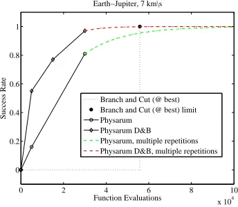
Earth−Jupiter, 7 km\s

Branch and Cut (@ best) Branch and Cut (@ best) limit Physarum

Physarum D&B

Physarum, multiple repetitions Physarum D&B, multiple repetitions

Fig. 5. Success rate: Physarum, Physarum D&B and Branch & Cut. Earth to Jupiter transfer EJ7,v_∞,L= 7km/s,α= 1.5π.

angle β = 1.5π, while the EJ7 has a departure velocity v_∞,L = 7 km/s and a departure angle β = 1.5π. The pericentre altitude for the swing-by’s of Mercury, Venus, Earth, Mars and Pluto is200km , while it is5 Jovian radii for Jupiter, 2 planetary radii for Saturn, and one planetary radius for Uranus and Neptune.

The parameters of the Physarum solver, for this and the following test case, were set as follows: m = 0.005, ρ = 0.0001, GF = 0.005, Nagents = 20, pram = 0.6, λ = 0, kexplosion = 5, Qmax = 30. For this and all the cases in the remainder of this papernshare=∞. Both the unidirectional and multidirectional algorithms were run for 200 times on each of the two problems for a number of function evaluations that ranged between 5000 and 100000. It is important to recall that one function evaluation is the evaluation of a single arc connecting two nodes in the search tree in Fig. 2.

The best solution found by both Physarum solvers is the sequence of planets EVVEMJ (Earth, Venus, Venus, Earth, Mars, Jupiter) both for EJ7 and EJ5 with cost 1.48 and 1.38years, and is in line with the results obtained with the exhaustive search presented in [1].

Table IV shows that the success rate for the multidirec-tional solvers is 10%higher, at 30000 function evaluations, and more than 20% higher, at 5000 function evaluations, than the unidirectional solver. Furthermore, the Physarum D&B algorithm is around 30% faster, thanks to the match-ing approach that rapidly combines and discovers optimal sequences.

Fig. 5 shows the success rate for the unidirectional, multidirectional and a deterministic branch & cut algorithm. The branch & cut algorithm builds the tree of sequences in a manner similar to the unidirectional solver but cuts branches when the partial value of the objective function is already above the best value of the objective function for a complete transfer. Fig. 5 shows that the success rate of the branch & cut algorithm is zero up to a minimum number of function evaluation after which it jumps to 1. The switching point from 0 to 1 is reached at around 55000 function evaluations while the Physarum algorithm finds good solutions for any number of function evaluations, with an 93% success at 30000 function evaluations.

The figures show also the extrapolated success rate of the two algorithms assuming that the algorithm is run multiple times for a constant number of function evaluations. The extrapolation is computed by considering the probability of success that the algorithm would have if it was launched multiple times for 30000 function evaluations each time. The probability of success is 1−pn

30, where the probability of

failure at 30000 function evaluations is p30 and n, in this

case, is the number of repetitions.

Note that, if each planet-encounter time pair was a city in a TSP, each planet could be revisited K times and NP planets were available per each encounter, then

the maximum length of a sequence would be KNP and

A= Departure Planet

B= First Swing-by Planet

TA

1= Departure Time

ǻș

1 A

A T

1 B

B T

2 B

B T

B j

B T

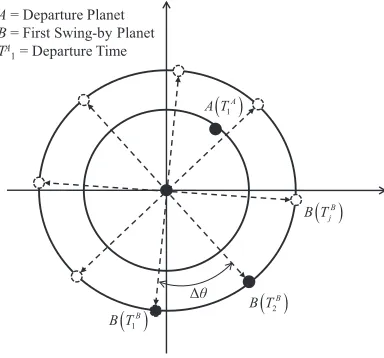
Fig. 6. Formulation in position for transfers between two planets.

V. MGAP 3D LAMBERTMODEL

In this section, the MGAP is modelled using the actual ephemerides of the planets. Given two planets,AandB, and the datesTA

i andTjB at which the spacecraft is at planetA andB, the solution of the Lambert’s problem gives the conic arc connecting the two planets and the associated velocity vectors at the beginning and at the end of the arc. IfB is a swing-by planet andCis the following planet in a sequence, the mismatch of velocity atBbetween the velocity vector at the end of theA-Barc (incoming velocity) and the velocity vector at the beginning of the B-C arc (outgoing velocity) is partially compensated by assuming that the gravity of the planetBis steering the incoming velocity. Since the altitude at which the spacecraft is allowed to swing-by the planet is limited and the mass of the planet is given, not all incoming velocities can be naturally rotated to match the outgoing velocities (i.e., the velocity difference between the velocity vector at the beginning of the arc following the swing-by and the velocity of the planet). In this case a propelled maneuver ∆vi is placed at the pericentre of the swing-by hyperbola. This combination of powered maneuver and gravity steering is called powered gravity assist manoeuvre or powered swing-by.

2) Formulation in Position: The position and velocity of the first planet in a sequence, sayA, are calculated from the ephemerides for the given vector of discrete times TA ₌ [T1A, T2A, ..., TiA, ...]

T_{. For all the subsequent planets, up the}

last one in the sequence, instead, the times are derived from the phase angles (see Fig. 6). AssumingBis the next planet in the sequence, followingA, andθB

1 is the phase angle ofB

on its orbit at timeTA

1 , the position, velocity and timeTjBof Bare computed forθB

j =θB1 + ∆θj, withj= 1, ..., nB and

nB = 2π/∆θj. The time corresponding to a given discrete phase angle can be computed from the time equation in the formTB

j =f(θBj + 2krπ). Note that, this model is applied also in reverse from the last planet to the first. In this case the position and velocity of the last planet are calculated from the ephemerides given a time vector that spans the desired arrival temporal window.

A. Generation of the Search Tree

If the vectors of encounter dates for planet A and B are respectively TA = [T₁A, T₂A, . . . , T_iA]T and TB = [TB

1 , T2B, . . . , TjB]T, then the set of possible transfers from

A to B can be represented with a matrix where each

element zAB

ij of the matrix is the cost associated with a particular T_iA→T_jB transfer. If multiple alternative planets are available the matrix becomes three dimensional, with the third dimension containing all possible planets. Note that each element of the matrix is a node in the tree of decisions that the Physarum incrementally builds, therefore only the nodes that the Physarum explores are actually generated and added to the tree. However, when a planet Athe Physarum generates a new branch towardsBall the transfers toB are evaluated and one selected to be added as a new node to the tree, the other transfers are stored for later addition of other nodes.

The costzAB

ij is the launch excess velocity∆v0if planet

Ais the departure planet, the powered swing-by cost∆vi if A is a swing-by planet, or the sum of ∆vi and the arrival excess velocity ∆vf ifB is the final planet. The cost of a complete transfer is then the sum of the departure∆v0plus

all the∆vi for all the planetary encounters and∆vf. In the Physarum algorithm, the variablesL(_totk)in Eq. (1) andLijin Eq. (6) are then replaced by, respectively,∆v_tot(k) andzAB

ij .

From a given planet at a particular node, a new planet is selected with a probability proportional to the inverse of the difference of the semimajor axis of the new planet with respect to the current one. Once the costs for the whole vector TB _{is available, a transfer is selected, for example} T2A→T2B, with Eq. (4), where only the costszABij are used to compute the fluxes. Ifν∈ U(0,1)> pram, the algorithm does not evaluate the cost for a new set of transfer arcs (i.e., does not build a new branch) but selects an existing arc among the available possibilities using Eq. (4). The process is repeated until the final target planet is reached and a complete decision sequence is built. If, during the construction of a solution, no transfer arcs can be found that satisfy the constraints, then the construction is terminated and an infinite cost (or equivalently a zero probability) is associated to the resulting partial solution. Eq. (6) was slightly modified by substitutingL(totk)withL

(k)

tot+ 1in order to avoid possible singularities that may appear with the MGA model.

1) Local Solution Improvement Strategy: In order to improve the quality of the solutions, a local search procedure inspired to the 2-optlocal search strategy was added to the algorithm. Ifs= [A, TA

2 , B, T7B, C, T12C, D, T16D]T is a

solu-tion vector, the local improvement checks whether a positive or negative increment of TA

2 , δT, improves the solution.

If, for example, ∆vtot(A, T2A, B, T7B, C, T12C, D, T16D) >

∆vtot(A, TA

2 +δT, B, T7B, C, T12C, D, T16D), then T2A is

re-placed by TA

2 +δT. The same δT is repeatedly added (or

subtracted) to TA

2 till no improvement is registered. The

process is then applied toTB

7 and the other dates tillT16D, and

2) Algorithm and problem settings: Along with the algorithm’s parameters m, ρ, GF, Nagents, pram, rini, kexplosionandλintroduced in Sec. II, a number of additional quantities needs to be defined to characterize a particular instance of the MGA problem. In particular, the departure planetP0, the upper and lower boundaries on the swing-by

altitude divided by the radius of the planethlowandhup, the set of available swing-by planets Ps={P1, P2, . . . , PNP},

maximum number of swing-by’snsmax, maximum number

of resonancesresmax, interval of dates defining the launch window Tlaunch, the interval of dates defining the arrival window Tarrival, the upper and lower boundaries on the time of flight T oFlow

ij and T oF up

ij for each leg connecting two planetsiandj, the final target planetPtarget, the grid spacing in angle∆θij and the upper and lower boundaries on launch and arrival velocities, respectively∆vmax

0 ,∆v0min

and ∆vmax f , ∆v

min

f . The settings of the algorithm for the cases in this and following section can be found in Tables V, VI. Planets are identified with the following let-ters Me(Mercury), V(Venus), E(Earth), M(Mars), J(Jupiter), S(Saturn), U(Uranus), N(Neptune), P(Pluto). For exam-ple the sequence EVVEJS means Earth-Venus-Venus-Earth-Jupiter-Saturn. Parameters m, ρ, GF, Nagents, pram are set with the same values used for the TSP and MGA 2D energy model examples (Sec. III and Sec. IV), whilstriniis increased from 1 to 2, andkexplosion consequently, in order to have a maximum radius of 5.

Note that, if, in this case, each planet-encounter time pair was a city in a TSP, each planet could be revisitedKtimes, NP planets were available per each encounter and each pair of planets required the evaluation of (NPKNT)2 transfer arcs, where NT is the number of discrete encounter dates, then the total number of transfers to be evaluated would be KNP(NPKNT)2_{. If the transfer arcs were put together in}

a sequence, the number of alternative sequences would be (KNP)(NPKNT)_.

B. Case Study: Mission to Saturn

This test case reproduces the Cassini mission, launched in November 1997 to Saturn [19]. For this particular example the maximum number of swing-by’s is 4 and the swing-by planet can be selected from a set of 4 planets with a maximum of2repeating planets in the same sequence. The code was implemented in Matlab⃝R _{R2010b. The simulation}

lasted for approximately 7 hours on an Intel Core (TM) i5-2500 3.30GHz. Table VII shows the top solutions for the sequences found by the Physarum: EVVEJS with a cost of 10.0873km/s, EVJS with a cost of10.5125km/s and EVVJS with a cost of 11.6184.

Table VIII shows a comparison between the best solution found by the Physarum solver working in only one direction versus, the best solution found by the Physarum solver with multidirectional matching ability and the solution found by the Hidden Genes solver proposed in [5]. This figure shows that the Physarum D&B is able to find the best solution. Not only does the multidirectional Physarum yield the best results but it also provides a more even spreading of the ∆vi maneuvers. In fact, the solutions found by incrementally building the sequences in only one direction (from Earth to Saturn) tend to have low costs at departure

and first by, with a higher cost at the second swing-by (approximately 2.6 km/s in the example in Table VIII); this is intrinsically due to the fact that any forward search algorithm (including deterministic branch and prune ones) is biased by the heuristic that is used to locally generate and select new branches. The parallel backward and forward search with intermediate matching completely removes this bias.

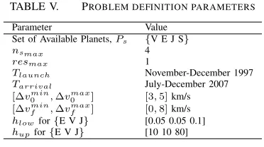
TABLE V. PROBLEM DEFINITION PARAMETERS

Parameter Value

Set of Available Planets,Ps {V E J S}

nsmax 4

resmax 1

Tlaunch November-December 1997

Tarrival July-December 2007

[∆v₀min,∆vmax₀ ] [3,5]km/s [∆v_fmin,∆vmax_f ] [0,8]km/s hlowfor{E V J} [0.05 0.05 0.1]

hupfor{E V J} [10 10 80]

TABLE VI. LOWER AND UPPER BOUNDARIES ON THE TIME OF FLIGHT AND∆θ

Me V E M J S

lb [day] 0 0 300 0 0 0 Me

ub [day] 0 0 1000 0 0 0 Me

∆θ[deg] 0 0 4 0 0 0 Me

lb [day] 0 100 30 300 500 0 V

ub [day] 0 500 500 2000 3000 0 V

∆θ[deg] 0 2 1 2 0.5 0 V

lb [day] 300 100 350 100 800 0 E ub [day] 1000 200 745 600 1500 0 E

∆θ[deg] 2 1.6 1 2 0.4 0 E

lb [day] 0 0 0 0 0 0 M

ub [day] 0 0 0 0 0 0 M

∆θ[deg] 0 0 2 2 0.5 0.52 M

lb [day] 0 0 0 0 0 1500 J

ub [day] 0 0 0 0 0 2900 J

∆θ[deg] 0 0 0 0 0 0.2 J

VI. CONCLUSIONS

This paper introduced a novel bio-inspired method for single objective discrete optimization that can effectively solve MGA trajectory problems. The algorithm was first applied to the TSP showing good performance if compared with ACS and other TSP specific algorithms. Furthermore, it was demonstrated that a multidirectional search is more efficient than a unidirectional search, when applied to the solution of reversible decision-making problems. The algo-rithm was then applied to two instances of the MGAP. In the first case the proposed algorithm showed the ability to quickly find optimal solutions for two variants of an Earth to Jupiter transfer, outperforming a classical unidirectional branch & cut technique.

TABLE VII. BEST THREE SEQUENCES FOR THECASSINI TEST CASE AT40000FUNCTION EVALUATIONS

Sequence Cost [km/s] Epoch [MJD2000]

EVVEJS 10.087 [₋779.160,₋595.763,₋181.432,₋132.692,463.099,2737.50] EVJS 10.512 [₋783.0,₋636.054,296.144,2765.595]

EVVJS 11.618 [₋766.960,₋585.780,₋164.193,483.760,2895.944]

TABLE VIII. CASSINI TEST CASE:COMPARISON BETWEEN UNIDIRECTIONAL,MULTI-DIRECTIONALPhysarum(BOLD)ANDHGGA (ITALICS)

E V V E J S

5/11/1997 2/4/1998 25/6/1999 20/8/1999 17/4/2001 25/10/2007 Date 13/11/1997 15/5/1998 4/7/1999 21/8/1999 8/4/2001 1/7/2007

30/11/1997 20/5/1998 26/6/1999 19/8/1999 24/3/2001 1/1/2007

148.3 448.5 55.7 606.8 2382.0

T oF 183.4 414.3 48.7 595.8 2274.4

[day] 171.5 402.0 53.8 582.6 2120.5

Pericentre 2554.8 19597.3 1609.3 4480675.7

Altitude 10484.0 872.2 2832.4 4638454.8

[km] 27471.0 605.3 1810.7 5167772.8

3.2893 0.2944 2.5265 3.3×10−4 3.4×10−3 4.2009 ∆v 3.9747 0.9502 0.9309 9.0×10−4 _5.6×10−4 _4.2298 [km/s] 3.7790 2.6330 1.1×10−5 1.4×10−6 1.9×10−4 4.2730

Total 10.3150

∆v 10.0873

[km/s] 10.6850

REFERENCES

[1] S Pessina, S Campagnola, M Vasile. Preliminary Analysis of Interplanetary Trajectories with Aerogravity and Gravity Assist Manoeuvres. 54th International Astronautical Congress, Bremen, Germany, 2003.

[2] A.E. Petropoulos, J.M Longuski, E.P. Bonfiglio. Trajectories to Jupiter via Gravity Assist from Venus, Earth and Mars. Journal of Spacecraft and Rockets, 37(6):776–783, 2000.

[3] M Vasile, P. De Pascale. On the Preliminary Design of Multiple Gravity-Assist Trajectories. Journal of Spacecraft and Rockets, 42(4): 794–805, 2006.

[4] M Ceriotti, M Vasile. Automated MGA Trajectory Planning with an ACO-inspired Algorithm. Acta Astronautica, 67(910): 1202-1217, 2010.

[5] A Gad, O Abdelkhalik. Hidden Genes Genetic Algorithm for Multi-Gravity-Assist Trajectory optimization. Journal of Spacecraft and Rockets, 48(4): 629–641, 2011.

[6] J.A Englander, B.A Conway, T Williams. Automated Interplanetary Trajectories Planning. AIAA/AAS Astrodynamics Specialist Confer-ence, Minneapolis, Minnesota, 2012.

[7] A Adamatzky, G.J Martinez, S.V Chapa-Vergara, R Asomoza-Palacio, C.R Stephens. Approximating Mexican Highways with Slime Mould.Natural Computing, 10(3): 1195–1214, 2011. [8] D.S Hickey, L.A Noriega. Insights into Information Processing by the

Single Cell Slime Mold Physarum Polycephalum. UKACC Control Conference, , Manchester, UK, 2008.

[9] T Nakagaki, H Yamada, A Toth. Maze-Solving by an Amoeboid Organism.Nature, 407(6803): 470, 2000.

[10] A Tero, K Yumiki, R Kobayashi, T Saigusa, T Nakagaki. Flow-Network Adaptation in Physarum Amoebae.Theory in Biosciences, 127(2): 89–94, 2008.

[11] A Tero, R Kobayashi, T Nakagaki. Physarum Solver: a Biologically Inspired Method of Road-Network Navigation.Physica: A Statistical Mechanics and its Applications, 363(1): 115–119, 2006.

[12] N Aras, BJ Oommen, IK Altinel. The Kohonen Network Incorporat-ing Explicit Statistics and its Application to the TravelIncorporat-ing Salesman Problem. Neural Networks, 12(9): 12731284, 1999.

[13] M Budinich. A Self-organizing Neural Network for the Traveling Salesman Problem that is Competitive with Simulated Annealing. Neural Computation, 8: 416424, 1996.

[14] M Dorigo, LM Gambardella. Solving Symmetric and Asymmetric TSPs by Ant Colonies. Proceedings of IEEE International Confer-ence on Evolutionary Computation,622-627, 1996.

[15] T Stuetzle, H Hoos. Max-Min Ant System and Local Search for the Traveling Salesman Problem. IEEE International Conference on Evolutionary Computation, 309-314, 1997.

[16] TSPLIB, library of instances for travelling salesman and vehicle routing problems, Ruprecht Karls Universitaet Heidelberg, URL: http://comopt.ifi.uni-heidelberg.de/software/TSPLIB95/.

[17] X. Zhang, L. Tang. A New Hybrid Ant Colony optimization Al-gorithm for the Traveling Salesman Problem. Advanced Intelligent Computing Theories and Applications: With Aspects of Artificial Intelligence, 148-155, 2008.

[18] Zar Chi Su Su Hlaing, May Aye Khine. Solving Traveling Salesman Problem by Using Improved Ant Colony Optimization Algorithm. International Journal of Information and Education, 1(5): 404-409, 2011.