Predicting visual function from the measurements of retinal nerve fiber layer structure

City, University of London Institutional Repository

Citation:

Zhu, H., Crabb, D. P., Schlottmann, P. G., Lemij, H. G., Reus, N. J., Healey, P. R., Mitchell, P., Holm, T. and Garway-Heath, D. F. (2010). Predicting visual function from the measurements of retinal nerve fiber layer structure. Investigative Ophthalmology and Visual Science, 51(11), pp. 5657-5666. doi: 10.1167/iovs.10-5239

This is the unspecified version of the paper.

This version of the publication may differ from the final published

version.

Permanent repository link:

http://openaccess.city.ac.uk/3332/

Link to published version:

http://dx.doi.org/10.1167/iovs.10-5239

Copyright and reuse: City Research Online aims to make research

outputs of City, University of London available to a wider audience.

Copyright and Moral Rights remain with the author(s) and/or copyright

holders. URLs from City Research Online may be freely distributed and

linked to.

City Research Online: http://openaccess.city.ac.uk/ [email protected]

Predicting Visual Function from the Measurements of

Retinal Nerve Fibre Layer Structure

Haogang Zhu,1 _{David P Crabb,}1 _{Patricio G Schlottmann,}2 _{Hans G Lemij,}3 _{Nicolaas J Reus,}3 Paul R Healey,4 Paul Mitchell,4 Tuan Ho,2 David F Garway-Heath2

1_{Department of Optometry and Visual Science, City University London, United Kingdom}

2_{NIHR Biomedical Research Centre for Ophthalmology, Moorfields Eye Hospital NHS}

Foundation Trust and UCL Institute of Ophthalmology, London, UK

3_{Glaucoma Service, The Rotterdam Eye Hospital, Rotterdam, Netherlands}

4_{Department of Ophthalmology, University of Sydney, Sydney, Australia}

Running Title: Zhu et al. Predict Visual Function from Retinal Structure

Key words: glaucoma, visual field, scanning laser polarimetry, Bayesian methodology, radial basis function, structure-function relationship

Corresponding author: David Crabb, Department of Optometry and Visual Science, City University London, Northampton Square, London, EC1V 0HB, UK. Phone: +44 (0) 2070400191; E-mail: [email protected]

Support: This research has been supported by Pfizer with an Investigator Initiated research grant; and has received a proportion of its funding from the Department of Health’s NIHR Biomedical Research Centre for Ophthalmology at Moorfields Eye Hospital and UCL Institute of Ophthalmology. The views expressed in the publication are those of the authors and not necessarily those of the Department of Health.

Abstract

Purpose: To develop and validate a method for predicting visual function from retinal nerve fibre layer (RNFL) structure in glaucoma.

Methods: RNFL thickness (RNFLT) measurements from GDxVCC scanning laser polarimetry (SLP) and visual field (VF) sensitivity from standard automated perimetry were made available from 535 eyes from three centres. In a training dataset, structure-function relationships were characterized using linear regression and a type of neural network: Radial Basis Function customised under a Bayesian framework (BRBF). These two models were used in a test dataset to 1) predict sensitivity values at individual VF locations from RNFLT measurements and 2) predict the spatial relationship between VF locations and positions at a peripapillary RNFLT measurement annulus. Predicted spatial relationships were compared with a published anatomical structure-function map.

Results: Compared with linear regression, BRBF yielded a nearly two-fold improvement (P<0.001; paired t-test) in performance of predicting VF sensitivity in the test dataset (mean absolute prediction error of 2.9dB (standard deviation (SD) 3.7dB) versus 4.9dB (SD 4.0dB)). The predicted spatial structure-function relationship accorded better (P<0.001; paired t-test) with anatomical prior knowledge when the BRBF was compared with the linear regression (median absolute angular difference of 15° versus 62°).

Introduction

Assessing the way in which structural and functional measures in glaucoma interact is clinically important. Visual loss is assumed to follow from, and correlate to, structural loss caused by the disease process. It would be clinically useful to know the magnitude and location of structural loss that will result in visually important functional loss. However, current clinical devices for measuring structural and functional deficits are far from accurate and have imperfect precision. Structural measures of optic nerve head (ONH) topography or retinal nerve fibre layer thickness (RNFLT) can be made using optical imaging techniques, but these only provide surrogate measures of the biological variable of real interest, namely retinal ganglion cell (RGC) count and function. At the same time, standard automated perimetry (SAP), the clinical cornerstone of functional testing in glaucoma, is subject to considerable measurement variability and is also a poor surrogate for RGC count and function.1 _{Despite their limitations, these techniques are currently central to the diagnosis and} management of glaucoma. It would, therefore, be beneficial if structure and function measurements were directly linked in some way, allowing clinicians to corroborate decisions by considering the measurements in tandem.

There have been several studies attempting to quantify the structure-function relationship using clinical measurements. These typically proceed by taking one summary value to represent function (for example Mean Deviation, MD, of the visual field from SAP) and one number to represent the structural data (for example, average neuroretinal rim area or mean RNFLT), then simply assessing the curve linear (e.g. log-linear) or monotonic association between the two variables via R2_{, Pearson or Spearman coefficients.}2-5 _{This approach suffers} from two major flaws: the use of summary data loses spatial information and may reduce power, and these association measures and regression models assume a particular shape of the relationship. Furthermore these analyses fail to take account of spatial associations in the data, an integral attribute of glaucomatous loss.

structure (pixel or sector values) and function (areas of VF or individual locations) are more likely to interact as ‘groups’ rather than single independent measurements.

In recent years, a special class of artificial neural networks using Radial Basis Functions (RBF) have received considerable attention.13-16 _{This class of networks differs from the} artificial neural networks (ANNs) that use a multilayer perceptron (MLP) approach, in that the nonlinearity of the model is embedded in a hidden layer of the network: this hidden layer consists of basis functions. The key element of the RBF is that predictions can be made in a multi-dimensional space that consists of ‘mini-distributions’ of possible predictions, analogous to a kernel or window when interpolating data. RBF networks are particularly useful when mapping two- or three-dimensional images where interpolation is a prerequisite, with some image features being preserved while others not necessarily being mapped exactly. In this way they seem most suitable to the problem of mapping the individual points from the structural and functional measures. Moreover, the RBF method developed for our purposes is formulated under a Bayesian probabilistic framework in order to tackle the considerable variability in measurements as well as to form an automatic learning process: this customisation leads to what we denote a Bayesian RBF (BRBF) network.

Methods

Subjects

The study sample was derived from three independently acquired populations from Moorfields Eye Hospital, London (MEH), Rotterdam Eye Hospital, the Netherlands (REH) and the Blue Mountains Eye Study, Australia (BMES)

Moorfields Eye Hospital (MEH) Data

Thirty-four healthy subjects (34 eyes), 43 glaucomatous patients (43 eyes) and 30 ocular hypertension subjects (30 eyes) were enrolled. Inclusion criteria for the healthy subjects were a normal VF, intraocular pressure (IOP) <21 mm Hg, no previous history of ocular disease, and no family history of glaucoma in a first degree relative. For the glaucomatous patients, inclusion criteria were previously raised IOP (>21mmHg), reproducible VF defects and absence of other disorders that might cause VF loss. The VF defects were defined as a defect of two or more contiguous points in the Humphrey pattern deviation probability maps with P <1% loss or greater, or three or more contiguous points with P <5% loss or greater, or a 10 dB difference across the nasal horizontal midline at two or more adjacent points in the total deviation plot. Ocular Hypertension subjects were recruited from clinic on having a raised IOP >21 mmHg in two consecutive visits and having at least two normal VFs. Optic disc appearance was not used to categorize subjects. However, the optic disc was evaluated to exclude anatomical abnormalities such as coloboma or drusen. For all participants, one eye was randomly selected for study if both were eligible. All subjects had visual acuity of 20/40 or better, with ametropia <7 diopters, and had no other significant ocular abnormality or concomitant ophthalmic condition.

Rotterdam Eye Hospital (REH) Data

Blue Mountains Eye Study (BMES) Data

VFs and images were available for 1540 subjects from a large population-based study of visual impairment, common eye diseases, and other health conditions from an elderly community in Australia. A description of the Blue Mountain Eye Study (BMES) is given elsewhere.19 _{Two hundred and thirty healthy subjects (230 eyes) and 76 patients (76 eyes)} diagnosed with glaucomatous optic neuropathy were selected from this population under strict measurement quality criteria (described below). Only one randomly selected eye per subject was used throughout. The criteria used for defining glaucomatous VF loss was an abnormal Humphrey Glaucoma Hemifield Test (GHT) plus one or more of the following VF defect classifications (top row of test points in 24-2 pattern were excluded to reduce the effect of lid artefact), which could not be explained on the basis of non-glaucomatous ocular, or neurological, causes: (1) at least 4 contiguous points on pattern deviation plot depressed at p<0.5% level; (2) at least two horizontal points in nasal step locations with pattern deviation plot depressed at p<0.5% level; (3) advanced glaucomatous field loss (hemispheric or severe generalised field loss, with residual temporal or central islands). Glaucoma was diagnosed if glaucomatous VF loss was present, combined with matching neural rim loss at the optic disc, and gonioscopy showed no evidence of angle-closure, rubeosis or secondary glaucoma, other than pseudoexfoliation syndrome.

All three datasets were collected in accordance with the tenets of the Declaration of Helsinki from studies that had local research ethics committee approval with all participants giving informed consent. Data were anonymized and transferred to a secure database held at City University London.

Measurements and Data

centres. The 64-sector thickness profile on the peripapillary annulus (provided by the GDx software) for each subject and the raw images (.mif files) were transferred to a secure database.

The VF measurements were acquired in all cases using a Humphrey Field Analyzer (HFA) II (Carl Zeiss Meditec, CA, USA) using either full-threshold testing or the Swedish Interactive Threshold Algorithm (SITA) Standard test program in the standard 24-2 test pattern. For the MEH and REH data, all VFs were considered reproducible as well as reliable. The VFs from MEH data were all tested with the SITA standard program. VF reliability indices applied were: fixation losses ≤15%; and false-positive and false-negative response rates ≤25%. In the REH data, 29 healthy subjects and 73 glaucomatous subjects were tested with the full-threshold program and the others with the SITA standard program. Reliability indices applied were: fixation losses ≤25%; and false-positive and false-negative response rates ≤20% for full-threshold test and ≤7% for SITA standard test. Higher false-negative response rates were accepted in eyes with advanced field loss (up to 33%). All VFs in BMES were tested with the full-threshold program. Stricter reliability criteria were applied: fixation loss, false positive and false negative all ≤15%. In all eyes, the two VF test points above and below the blind spot were excluded and the remaining 52 raw (dB) sensitivity values (dB) were transferred to a secure database for analysis.

In this study, the MEH and REH datasets (229 eyes in total) were used for development of the models, and the BMES dataset (306 eyes in total) was used for independent testing in order to demonstrate the generalization of the method. The image and VF quality criteria were used only for the purpose of selecting reliable measurements and were not used in the modelling. Moreover, the proposed model does not need the initial labelling of the subject data as being from glaucomatous or healthy eyes, and under the Bayesian framework, no manual input parameters are required.

Statistical Models

What follows is a description of the principal methods and models developed. Technical and mathematical details can be found elsewhere22 and are reviewed in the Appendix. The BRBF model was developed and written in Matlab (version 7.4.0 R2007a, The MathWorks, Inc., Natick, MA). An executable version of this code is freely available from the authors.

allow the prediction of a VF sensitivity value from RNFLT values and vice versa. The remaining part of this section compares the BRBF model to the linear model that has been used widely to assess the association between structural and functional measurements.

Starting with a linear model, consider the case where we attempt to predict an individual VF

sensitivity value denoted ˆy_d (where dis one of the 52 locations in a 24-2 HFA VF) from a

series of RNFLT values denoted x_i for i from 1 to m. This can be expressed by the following

over-simplified but illustrative equation:

1 1 2 2

ˆ_d  _d  _d  ... _{dm m}c_d

y w x w x w x (1)

where c_d is a constant offset. The symbol on ˆy_d indicates that it is a prediction rather than

the real measured value denoted by y_d. In this example, the equation has 64 peripapillary thickness profile values (m=64) each with its own coefficient which quantifies the

contribution of each x value to the prediction. So each y value can be predicted by a ‘linear

combination’ of x values. With some actual data we can find some real numbers for the w

terms by least squares regression; this attempts to ‘fit’ an equation that minimises the difference between the predicted and measured values. This yields an individual equation for each y that can be enumerated across all the points to predict a complete VF from a given

vector of x values. This classic multiple linear regression can be adapted to select only those

x values that are statistically significant for the prediction of yvalues using techniques such

as stepwise multiple regression23 with the forward selection scheme. In a linear model described by equation (1), the w values (divided by their standard errors) quantify the amount of meaningful contribution made by x values to predict the y values. The largest

absolute w term (with respect to the variability in estimating the term) would indicate the x

value that affects the y_d value the most, in the sense that change in this x value results in the largest change in y_d. Similarly, the next largest absolute w term would indicate the second most important term and so on. Equivalently, one could look at the relationship between the

d

y value and each x value separately and simply calculate the correlation coefficient based

from this model was converted back to the decibel scale when compared with the measured sensitivity. We will refer to this method as a classic linear model.

This ‘classic linear model’ approach makes several restrictive and incorrect assumptions about the data. First it assumes that each x value is independent of all the other x values,24 whereas in reality the x and y values are topographically and physiologically related and

may interact as groups. Although one could try to demarcate these groups based on a physiological relationship between the x values, or an anatomical map, it would be preferable for the groups to be ‘learnt’ from the data rather than imposing any relationship from incomplete prior knowledge. Second, this approach assumes that the relationship between y

and x is either linear or linear after some transform (typically logarithmic). In reality, the relationship between y and x may be more complex with the nature of the association

probably changing across the measurement range of y. Put simply, at different stages of

disease, the apparent relationship between y and x could switch from being linear, to noisy,

to curvilinear and occasionally being censored due to the imprecision and range of the measurement. This notion that the association maychange at different levels of functional loss was also asserted by published studies.25, 26 _{The third difficulty with the classic linear} model is that outlier points exert an overly strong influence, and can yield a false association.

The RBF attempts to model the relationship between y and x without the limiting

assumptions associated with the classic linear model described above. As an illustrative

example, consider one x value, say x₁, appearing to be co-related to a y value, say y₁. This

apparent relationship might be explained by x₁ being very strongly related to x₂which in turn

is very strongly associated with y₁. Thus the apparent x₁ and y₁relationship may well be

much weaker or not even be significant. As it will be shown in the derived structure-function relationship (Figure 3-Figure 5), this covariance in the relationship between the y and x

'isolated' and will not affect the prediction. Moreover, RBF ‘learns’ the parameters from the data and this is customised for our purpose by using a Bayesian framework (BRBF). The method makes predictions in multiple dimensions by extending the standard relevance vector machine27 _{where the output is restricted to one dimension. The VF sensitivities at different} locations are implicitly correlated by sharing the same basis functions and parameters of weights (See α in the Appendix). In the BRBF model, the original visual field sensitivity value in dB was used.

In general, BRBF is not restricted by the number of inputs in the model, or more precisely by the dimensionality of the data, so that it can be adapted to use the RNFLT values at each pixel, rather than only the 64-sector peripapillary thickness profile. In this study, examples of the SLP images used for predicting VF are shown in Figure 2. We used an annular region, centred on the ONH. The inner and outer diameters were 2.3mm and 4.9mm, respectively, so that the annulus was 26 pixels wide (compared with the 8-pixel calculation ring in the GDx software from which the 64-sector RNFLT peripapillary profile is computed). In this annulus, there are 16512 pixels each with a retardation value. We hypothesised that the predicted spatial structure-function relationships would be strengthened by avoiding the data reduction to 64 sector RNFLT values. This hypothesis will be validated by the improved structure-function relationship derived from the BRBF by using the measurement in its higher dimensional form.

Another challenge in the modelling process involves handling the large dimensionality of the SLP data. If the dimensionality M and the number of data points N of a dataset satisfy MN, the dimensionality of the dataset can be reduced from M to N 1 with minimal loss of information using Principal Component Analysis28 _{(PCA), because the N data points span at} least one linear hyperplane in this M-dimensional space. Using this technique the 16512

dimensional SLP image vectors were reduced to 227 dimensions for analysis and transformed back to the original SLP vectors for the purpose of visualization and evaluation of results. Using the classic linear model on a reduced SLP image vector with 227 elements and a 24-2 VF with 52 sensitivity values will still result in a prohibitive number of ‘weights’ (11856) to be fitted, which will cause significant overfitting to the ‘noise’ in the data.

Testing the Model

developing a model, the input variables and weights selected may vary across different samples31_{. Therefore, the models were developed on the MEH and REH data alone, leaving} the BMES data as a test dataset.

The predictive performance of the classic linear model and the BRBF was evaluated by point-by-point analysis of the predictions of the VF sensitivity in the 306 VFs from the BMES dataset. The predictive performance was summarised by the mean of the absolute prediction errors in the 52 points of the VF.

Matlab code was written to display the results and present the output of the linear and BRBF models via a graphical user interface. One graphical output was a structure-function map in a similar format to that described by Gardiner et al (2005).9 The structure-function relationship was defined by the corresponding functional change given a subtle structural change, which is mathematically modelled by the derivative of the BRBF (Appendix). This describes the relationship between y (VF sensitivity) and x(RNFLT) at each individual VF location. The

other output from this analysis consisted of point-by-point predictions of each subject’s VF as represented by the HFA greyscale (which was replicated for this purpose). These outputs were considered for 1) the classic linear model, 2) the BRBF I model (based on the 64 summary RNFLT values output from the GDx software) and 3) for the BRBF II model (based on the reduced 227 dimensional data derived from the PCA on the 16512 individual pixel retardation values in the broad annulus centred on the ONH).

Results

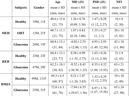
A summary of the measurements: HFA mean deviation (MD), HFA pattern standard deviation (PSD); GDx Nerve Fibre Indicator (NFI)) for each of the datasets is given in Table 1.

The mean absolute prediction error of VF sensitivities in the 306 eyes from the BMES data was 4.9dB (standard deviation (SD) 4.0dB) for the classic linear model. In comparison, both BRBF models yielded a nearly two-fold improvement (P<0.001; paired t-test) in performance: BRBF I 2.9dB (SD 3.7dB), BRBF II 2.8dB (SD 3.8dB). In BRBF I and BRBF II models, the training process described in Appendix selected 49 and 73 basis functions respectively in the hidden layer.

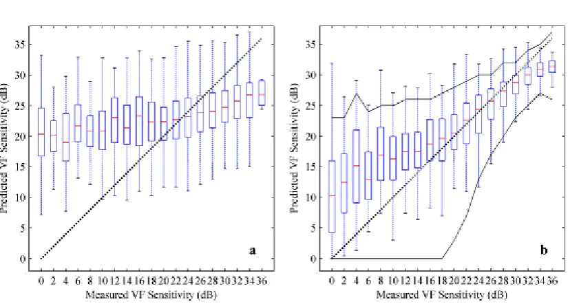
limits)32 _{across all locations from two VF tests from each of 49 individuals have been} superimposed on Figure 1b. On inspection, these limits are similar to the 90% prediction limits when using the BRBF to predict the VF from a GDx RNFLT measurement of the same individual. Note that predictions at higher sensitivities (>30dB) tend to be slightly lower than the actual values whilst at lower sensitivities (<20dB) the predictions tend to be higher.

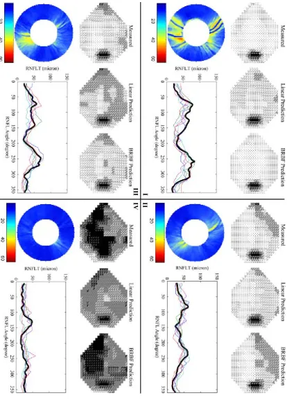
Figure 2 gives some case examples of the predictions. In some cases, the classic linear model overestimates the defect severity of the VF (I and III) and in other cases predicts a less damaged VF (IV), when compared to the true measured VF. In Figure 2(II) the classic linear model matches the overall average sensitivity of the VF but fails to capture the spatial location of this loss. In each case the BRBF better estimates the true VF, with spatial features of the measured defects generally retained. In Figure 2(IV) the BRBF model manages to predict the advanced defect severity.

Figures 3, 4 and 5 provide topographical maps of the spatial relationship between RNFLT positions on the peripapillary annulus and VF sensitivity at all the points in the VF, by means of classic linear regression, BRBF I and BRBF II, respectively. The agreement between the derived structure-function relationship and the anatomical benchmark was also summarised by calculating the absolute angular difference between the direction with the strongest derived relationship and the anatomical benchmark. This was calculated as the median of the absolute angular difference across all locations in a spatial relationship map such as Figures 3, 4 and 5. Both visual inspection on the spatial relationship and the quantified agreement with anatomical prior knowledge showed that the structure-function relationship derived by the classic linear regression model (Figure 3) has little concordance (median absolute angular difference of 62°) with the anatomical benchmark.33 This correspondence improves (P<0.001; paired t-test) with the BRBF I model (median absolute angular difference of 15°) in general, and improves further (P<0.001; paired t-test) still with the BRBF II model (median absolute angular difference of 12°), especially at the points around central vision and blind spot. This is consistent with the BRBF models learning to 'encode' the structure-function relationship during the training.

Discussion

the prediction of the output, which makes them combine and interfere with each other. This typically yields a highly non-linear training process with mathematical difficulties that result in a slow convergence of a training procedure16_{. Moreover, the complexity of hidden unit} patterns causes difficulty when interpreting the result because the connection among units and the hidden unit output do not have any physical or realistic meaning: they are simply some numbers that can produce a correct output. Hence, MLP ANNs are less suitable for the mapping of points in different measurement spaces, which requires a detailed understanding of the hidden layer output and other manipulation (e.g. derivatives) within the network. In this study, although an MLP provided a prediction accuracy comparable to the BRBF (data not shown), the spatial aspects of the structure/function relationship were poorly predicted. This likely results from complex interactions among the large number of weights in the MLP model. In contrast, RBF substitutes hidden layers in MLP with a set of basis functions, which leaves the solution of weights in a linear space. The Gaussian basis function forms a local representation in the hidden unit, each of which can be understood as a representative of similar input patterns (Figure 2). With a given RNFLT input, only a few ‘representatives’ will be activated and contribute to the VF prediction (Figure 2). Furthermore, the RBF handled within a Bayesian probabilistic framework,27 _{as developed for our purposes, is unlike} most other ANN approaches because it is independent of any subjective input parameter, and thus requires no model validation on a test dataset provided that the training dataset is representative and sufficiently large to enable modelling of the many different states of the VF. However, for this study the ‘trained’ model is still tested on a separate, independent dataset to illustrate the generalisation of the model performance. One ‘technical’ limitation of the current BRBF model, despite its good performance, is that it assumes that the variability in the VF measurements is largely Gaussian, which is not optimal given that it is often skewed and heavily-tailed.32

A plausible explanation for the improvements afforded by the BRBF technique is that it models the spatial and quantitative structure-function relationship more precisely. The technical and statistical advantages of the BRBF model over the classic linear model would support this notion. For example, the BRBF considers that the VF points, and indeed RNFLT values acquired from different discreet areas, interact as groups rather than as independent measurements. The BRBF also accommodates the covariance and non-independence of the measurements; it is less affected by outlying observations and makes no assumption about the linearity of relationships. Of course, one difficulty in generating any type of map, driven by data or anatomical observation, is the restriction in the sampling of VF points: these are, for example, probably not optimally placed for estimating RGC density nearer the fovea.

The range and distribution of differences between the measured VF sensitivity values and those predicted from the RNFLT by the BRBF, at different levels of sensitivity, is shown in Figure 1b. This profile is remarkably similar to published limits for test retest variability when two VFs are measured within a short space of time.32 _{This suggests that, on average, a} VF predicted by the BRBF from RNFLT values has measurement noise equivalent to that found in a newly measured field. This isn’t as exciting as it may first appear because it is well established that the measurement noise in VFs is already very high, prohibiting straightforward clinical diagnosis of glaucomatous defects and monitoring progression. Nevertheless, this finding illustrates that the range and scale of the average predictive performance of the BRBF model is much better than the classic linear model approach, which completely fails to predict the full range of VF values (Figure 1a).

dataset may have ‘super-normal’ structure and the glaucomatous subjects have greater than average structural damage. This potential bias on subject selection might distort the structure-function relationship. Therefore, the training process may be improved by including a range of glaucoma severity in subjects defined only by VF loss. Another factor that may confound the reported prediction accuracy is that the models were trained with VFs tested with both SITA and threshold programs, while they were evaluated on VFs tested only with full-threshold program. This may, in part, account for the observed tendency for the prediction to overestimate the sensitivities in the test dataset due to the higher sensitivities obtained with SITA compared with the full-threshold program.44 _{However, this effect would be small} because the sensitivity difference with two programs is just 1.3dB on average.44

Recent investigations attempting to uncover the structure-function relationship in glaucoma generally have the aim of assessing the relativeaccuracy of structural and functional tests throughout the course of the disease45, 46_{. For example, loss of function without loss in} structure that does not adhere to a particular structure-function model’s prediction might be an indicator of a non-glaucomatous process, measurement imprecision, or some artefact in the image of the structure or function test. Our long term aim is to use the BRBF technique to provide a relevant clinical tool that indicates concordance between the VF and the chosen surrogate measure for structural loss. For example, when a VF and structural measure derived from one of GDx, HRT or optical coherence tomography (OCT) is available, a chart mapped in VF space will be provided indicating areas where the measurements are in concordance (within a certain range of accuracy and precision) and where they are not: this could provide clinically useful information about the reliability of the individual measurements or diagnostically useful information.

It is an imperative that any new statistical method should be developed and tested on more than one dataset.30 _{We had access to three large independent datasets, each collected at one of} three clinical centres. The inclusion criteria for glaucomatous and healthy subjects were generally consistent across the three samples. However, as the aim of this study was not to determine diagnostic performance, the precise definitions for glaucoma were less important. In fact, the mixture of data can be viewed as an advantage in the study design. However, further testing on different datasets, especially where realistic estimates of measurement precision have been performed (from test-retest measurement), is still required and this is being undertaken in our laboratory and elsewhere.

values) as well as the PCA-reduced RNFLT values at 16512 pixels in a wide peripapillary annulus. The BRBF method could be used on neuroretinal rim area values from SLO technology or RNFLT values derived from OCT technology, or any other surrogate measure of glaucomatous structural loss. Moreover, we have demonstrated, albeit qualitatively with the maps in Figure 5, that using the surrogate measures of RNFLT in their high dimensional form provides a closer mapping to the expected structure-function relationship. We speculate that the next generation of Fourier domain OCT instrumentation, now finding its way into clinics and providing volumes of data for RNFLT, will be particularly amenable to this method.

In conclusion, we have introduced a new statistical method for describing the relationship between functional and structural measurements used in the clinical evaluation of glaucoma. Evidence from a dataset independent of those used to derive the model indicates that the BRBF method has advantages over standard statistical approaches for modelling these relationships, and estimates of functional deficits from structural measures yielded from this method are better than those derived from a classic linear regression approach. This method can provide a platform from which clinically useful tools can be derived for mapping and charting concordance between VF measurements and RNFLT measurements in glaucoma.

Appendix

Our proposed method to link the structural and functional measurements is formalized by a function G, which would predict functional measurement y from a structural one x :

y =G( x ). This sets a mathematical framework for the question: what would be the

corresponding functional change (y) for the structural change x: y= (G x  x) G( )x ?

Because we are interested in subtle structural change to model the slow progression of RNFL damage, we assume that x becomes very small and tends to 0. The structure-function relationship is then defined with the general equation:

0

Lim

 

 

x

y x= 0

( ) ( )

Lim

 

   

x

x x x

x

G G _=

xG (2)

where G is differentiable w.r.t. x, and _xG is the gradient of G at x. Since we are sampling

subjects rather than considering the whole population, the final term in this equation must be

expressed as a statistical expectation of _xG or, for simplicity, the mean of _xG .

We examined classic linear regression and BRBF as the choice of function G. The latter was

one-dimensional. The extension was similar to the model derived by Thayananthan et al (2006).47 _{In particular, VF sensitivity is assumed to be:}

T _{( )}

n n

d  d d

y w x (3)

where n d

y is the dth element in the measurement of the nth subject, _xn _{is the RNFLT}

measurement (64-point profile or SLP image) vector, w_d is a weight vector, _d is an additive

zero-mean Gaussian noise _{(0, )}2

d



N with variance 2

d

 , and the radial basis function

vector ( )_xn _{is defined to be M+1 dimensional for M bases:}



1 ( )n 1, ( ),n

 x   x



2( ),..., ( )n M n

 x  x , where each element is a radial basis function with centre _m and an

isotropic covariance:



 







( ) expn n n

m m m m

 x   x   x  (4)

If all weight vectors w_d are organized into a matrix W columnwise, then using Bayesian methodology we assign a prior over W:

~ (0, )

d 

w N 　and　 ( | ) (0, )

d

p W  



N  ₍₅₎

where  is a diagonal matrix whose elements are 1 1 ,

 1 1

2 ,..., M

  _{on diagonal and 0}

otherwise. Each 1

m

 _{represents the average variance of the weights for the}

mth basis.

According to Bayesian methodology, priors of hyper-parameters are defined over _m and 2

d d

 _  _:

( ) Gamma( _m| , )

m

p  



 a b , ( ) Gamma( _d| , )

d

p  



 c d ₍₆₎

where α and β are vectors of _m and _d respectively, and Gamma(_m| , )a b is a Gamma

distribution with parameters a and b.

The framework above forms the objective function, which is the probability of all parameters, , ,

W α β, given the observations Y:

( , , | ) ( | , , ) ( , | )

where Y is a matrix, the columns of which are _yn _for

n from 1 to N.

In the first item in equation (7), it is straightforward to infer that w_d is independent from any other weight vectors given Y, α and β. Consequently:

( | , ) ( | )

( | , , )

( | , )

d d d d

d d d

p p

p

p

 





y w w α

W Y α β

y α ( d, d)

d







_{N w} _{w (8)}

where the covariance matrix and mean for the posterior distribution of w_d are:



₁



1

( ) ( )

d d



 

 _w  X  X   and ( )

d d d d

 _{  } 

w w X y (9)

where ( ) X is a matrix: ( ) X =



_{( ), ..., (x}1  _xN₎



T_.

The latter item in equation (7) can be calculated as: ( , | )p α β Y  p( | , ) ( ) ( )Y α β p α p β , where

( | , ) ( | , ) ( | )

p Y   



p Y W  p W  dW

1

1

... ( | , ) ( | ) ...

D

d d d d D

d

p  p  d d



_{ }



w w

y w w w w

_{(0, ( )}1 _{( ) )}

d d

I

  





N   X  X ₍₁₀₎

With no prior knowledge on α and β, these two parameters are assumed to be “uniformly”

distributed so ( )p α and p( )β have little impact on p( , | )α β Y . Using the similar

approximation as that of RVM,27 _{the hyper-parameters are optimized by setting the derivative} of equation (10) to be zero:

2

(( ) )

d d

m m mm

d D     



w w

and



 



(1 ) ( ) ( ) d d d mm m m d d d N             



w w w

y X y X (11)

where

d

m

_w is the mth element of the vector d

_w , and

d

mm

_w is the diagonal element at mth row

and column in

d

_w .

The parameters are inferred by iterating between equations (9) and (11) until convergence.

The radial basis centres _m are initialized to contain all _xn_{. As with an RVM, many of} m

become infinite during the training process, so the corresponding radial bases are removed

accordingly. The radial basis parameter _m is optimized by gradient descent.

Given the inferred parameters, the distribution of predicted values y_d given a test example x

is computed as:

(p y y_d| _d, , )α β

( _d | _d, ) ( _d | _d, , ) _d

p  p d



_

y w β w y α β w

T 1

( ( ), ( ) ( ))

d d d

  _    _  _

N _w x  x _w x (12)

where the prediction is made by the mean of the distribution: T _{( )}

d

 _w x .

Therefore, the structure-function relationship in equation (2) is implemented by

T ( )

d n n    w x x (13)

where ( )_nn

 

x x

1( )n _,..., M( )n

n n            x x

x x , and

( )n m

n

 

x

x is a vector: 2 ( )( )

n n

m m m

  

 x x 

1. Anderson RS. The psychophysics of glaucoma: Improving the structure/function relationship. Prog Ret Eye Res 2006;25:79-97

2. Brigatti L, Caprioli J. Correlation of visual field with scanning confocal laser optic disc measurements in glaucoma. Arch Ophthalmol 1995;113(9):1191-1194.

3. Weinreb RN, Shakiba S, Sample PA, et al. Association between quantitative nerve fiber layer measurement and visual field loss in glaucoma. Am J Ophthalmol

1995;120:732-738.

4. Iester M, Mikelberg FS, Courtright P, Drance SM. Correlation between the visual field indices and Heidelberg retina tomograph parameters. J Glaucoma 1997;6(2):78-82.

5. Teesalu P, Vihanninjoki K, Airaksinen P, Tuulonen A, Laara E. Correlation of blue-on-yellow visual fields with scanning confocal laser optic disc measurements. Invest Ophthalmol Vis Sci 1997;38:2452-2459.

6. Garway-Heath DF, Holder GE, Fitzke FW, Hitchings RA. Relationship between

Electrophysiological, Psychophysical, and Anatomical Measurements in Glaucoma. Invest Ophthalmol Vis Sci 2002;43:2213-2220.

7. Garway-Heath DF, Viswanathan A, Westcott M. Relationship between perimetric

light sensitivity and optic disc neuroretinal rim area. In: Wall M, Wild JM (eds), Perimetry Update 1998/1999. The Netherlands: Kugler Publications The Hague; 1999:381-389.

8. Anton A, Yamagishi N, Zangwill L, Sample P, Weinreb R. Mapping structural to

functional damage in glaucoma with standard automated perimetry and confocal scanning laser ophthalmoscopy. Am J Ophthalmol 1998;125(4):436-446.

9. Gardiner SK, Johnson CA, Cioffi GA. Evaluation of the Structure-Function

Relationship in Glaucoma. Invest Ophthalmol Vis Sci 2005;46:3712-3717.

10. Mai TA, Reus NJ, Lemij HG. Structure-Function Relationship Is Stronger with

Enhanced Corneal Compensation than with Variable Corneal Compensation in Scanning Laser Polarimetry. Invest Ophthalmol Vis Sci 2007;48:1651-1658.

11. Bowd C, Zangwill LM, Medeiros FA, et al. Structure and Function in Glaucoma: The Relationship between a Functional Visual Field Map and an Anatomic Retinal Map. Invest Ophthalmol Vis Sci 2006;47:2889-2895.

12. Schlottmann PG, Cilla SD, Greenfield DS, Caprioli J, Garway-Heath DF.

Relationship between Visual Field Sensitivity and Retinal Nerve Fiber Layer Thickness as Measured by Scanning Laser Polarimetry. Invest Ophthalmol Vis Sci 2004;45:1823-1829.

13. Powell MJD. Radial basis functions for multivariate interpolation: A review. In: Mason JC, Cox MG (eds), Algorithms for the approximation of functions and data: Clarendon

Press; 1987:143-167.

14. Orr MJL. Introduction to Radial Basis Function Networks. 1996.

15. Poggio T, Girosi F. Networks for approximation and learning. Proceedings of the IEEE 1990;78:1481-1497.

17. Reus NJ, Lemij HG. Relationships between Standard Automated Perimetry, HRT Confocal Scanning Laser Ophthalmoscopy, and GDx VCC Scanning Laser Polarimetry.

Invest Ophthalmol Vis Sci 2005;46:4182-4188.

18. Keltner JL, Johnson CA, Cello KE, et al. Classification of visual field abnormalities in the ocular hypertension treatment study. Arch Ophthalmol 2003;121:643-650.

19. Mitchell P, Smith W, Attebo K, Healey PR. Prevalence of open-angle glaucoma in Australia. The Blue Mountains Eye Study. Ophthalmology 1996;103:1661-1669.

20. Greenfield D. Optic nerve and retinal nerve fiber layer analyzers in glaucoma. Curr Opin Ophthalmol 2002;13:68-76.

21. Reus NJ, Colen TP, Lemij HG. Visualization of localized retinal nerve fiber layer defects with the GDx with individualized and with fixed compensation of anterior segment birefringence. Ophthalmology 2003;110:1512-1516.

22. Zhu H, Crabb DP, Garway-Heath DF. A Bayesian Radial Basis Function Model to

Link Retinal Structure and Visual Function in Glaucoma. The 3rd International Conference of Bioinformatics and Biomedical Engineering. Beijing: IEEE; 2009:1-4.

23. Hocking RR. The analysis and selection of variables in linear regression. Biometrics

1976;32:1-49.

24. Cohen J. Multiple Regression as a general data-analytic system. Psychological Bulletin 1968;70:426-443.

25. Harwerth RS, Carter-Dawson L, Smith EL, Crawford ML. Scaling the

structure-function relationship for clinical perimetry. Acta Ophthalmol Scand 2005;83:448-455.

26. Gonzalez-Hernandez M, Pablo LE, Armas-Domingue K, Vega RR, Ferreras A, Rosa

MG. Structure-function relationship depends on glaucoma severity. Br J Ophthalmol

2009;Epub ahead of print.

27. Tipping ME. The Relevance Vector Machine. In: Solla SA, Leen TK, Muller KR

(eds), Advances in Neural Information Processing Systems: MIT Press; 2000:652-658.

28. Jolliffe IT. Principal Component Analysis: Springer Press; 1986.

29. Copas JB. Regression, prediction and shrinkage (with discussion). J Roy Stat Soc B Met 1983;45:311-354.

30. Altman DG, Royston P. What do we mean by validating a prognostic model.

Statistics in Medicine 2000;19:453-473.

31. Miller AJ. Selection of subsets of regression variables (with discussion). J Roy Stat Soc A Sta 1984;147:389-425.

32. Artes PH, Iwase A, Ohno Y, Kitazawa Y, Chauhan BC. Properties of Perimetric

Threshold Estimates from Full Threshold, SITA Standard, and SITA Fast Strategies. Invest Ophthalmol Vis Sci 2002;43:2654-2659.

33. Garway-Heath DF, Poinoosawmy D, Fitzke FW, Hitchings RA. Mapping the visual

34. Bowd C, Chan K, Zangwill LM, et al. Comparing Neural Networks and Linear Discriminant Functions for Glaucoma Detection Using Confocal Scanning Laser Ophthalmoscopy of the Optic Disc. Invest Ophthalmol Vis Sci 2002;43:3444-3454.

35. Goldbaum MH, Sample PA, White H, et al. Interpretation of automated perimetry for glaucoma by neural network. Invest Ophthalmol Vis Sci 1994;35:3362-3373.

36. Bengtsson B, Bizios D, Heijl A. Effects of Input Data on the Performance of a Neural Network in Distinguishing Normal and Glaucomatous Visual Fields. Invest Ophthalmol Vis Sci 2005;46:3730-3736.

37. Brigatti L, Hoffman D, Caprioli J. Neural networks to identify glaucoma with structural and functional measurements. Am J Ophthalmol 1996;121:511-521.

38. Uchida H, Brigatti L, Caprioli J. Detection of structural damage from glaucoma with confocal laser image analysis. Invest Ophthalmol Vis Sci 1996;37:2393-2401.

39. Brigatti L, Nouri-Mahdavi K, Weitzman M, Caprioli J. Automatic detection of

glaucomatous visual field progression with neural networks. Arch Ophthalmol

1997;115:725-728.

40. Spenceley SE, Henson DB, Bull DR. Visual field analysis using artificial neural networks. Ophthalmic and Physiological Optics 2007;14:239-248.

41. Wyatt HJ, Dul MW, Swanson WH. Variability of visual field measurements is

correlated with the gradient of visual sensitivity Vision Research 2007;47:925-936.

42. Blumenthal EZ, Horani A, Sasikumar R, Garudadri C, Udaykumar A, Thomas R.

Correlating Structure With Function in End-Stage Glaucoma. Ophthalmic Surg Lasers Imaging 2006;37:218-223.

43. Yanagisawa M, Tomidokoro A, Saito H, et al. Atypical retardation pattern in

measurements of scanning laser polarimetry and its relating factors. Eye 2009;23:1796-1801.

44. Sharma AK, Goldberg I, Graham SL, Mohsin M. Comparison of the Humphrey

swedish interactive thresholding algorithm (SITA) and full threshold strategies. Journal of glaucoma 2000;9:20-27.

45. Hood DC, Anderson SC, Wall M, Kardon RH. Structure versus Function in

Glaucoma: An Application of a Linear Model. Invest Ophthalmol Vis Sci 2007;48:3662-3668.

46. Hood DC, Kardon RH. A framework for comparing structural and functional

measures of glaucomatous damage. Prog Ret Eye Res 2007;26:688-710.

47. Thayananthan A, Navaratnam R, Stenger B, Torr PHS, Cipolla R. Multivariate

Subjects Gender Age

meanSD (min, max)

MD (dB) meanSD (min, max)

PSD (dB) meanSD (min, max)

NFI

meanSD (min, max)

MEH

Healthy 19M, 11F 40.615.6 (21, 75)

1.260.76 (0.09, 3.30)

1.470.28 (1.12, 2.27)

168 (2, 30)

OHT 13M, 21F 60.711.1

(21, 75)

1.070.82 (0.10, 3.06)

1.350.27 (1, 2.1)

2010 (5, 43)

Glaucoma 28M, 15F 60.813.1 (31, 84)

-4.022.55 (-12.00, 1.15)

4.932.93 (1.49, 12.50)

4218 (11, 80)

REH

Healthy 23M, 23F 60.412.1 (23, 77)

0.380.99 (-1.55, 2.73)

1.630.26 (1.13, 2.30)

219 (2, 43)

Glaucoma 47M, 29F 62.210.1 (30, 82)

-9.528.43 (-30.39, 1.25)

8.354.32 (1.99, 15.92)

6321 (21, 98)

BMES

Healthy 99M, 131F 69.36.5 (60, 87)

0.211.07 (-1.26, 3.03)

1.530.29 (1.12, 2.55)

1910 (2, 49)

Glaucoma 25M, 51F 72.06.3 (61, 78)

-7.946.55 (-29.67, 1.56)

6.973.76 (1.67, 15.56)

[image:24.595.80.516.102.428.2] [image:24.595.83.515.105.424.2]

6524 (27, 98)

[image:25.595.91.504.96.317.2]

List of Figures

[image:26.595.92.507.70.649.2]

[image:27.595.92.503.221.566.2]

annulus from the GDxVCC scanning laser polarimetry (SLP) images was in general similar to the one from BRBF I. The row of graphics below show the GDxVCC SLP image annulus and the corresponding 64-sector retinal nerve fibre layer thickness (RNFLT; thick black line) used to predict the VFs. The coloured lines in the 64-sector RNFLT plot indicate the top five radial basis functions with the strongest activation (those contributing the most to the prediction). More examples have been provided as supplementary material for this article.

[image:28.595.93.504.70.409.2]

[image:29.595.93.504.70.409.2]

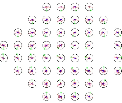
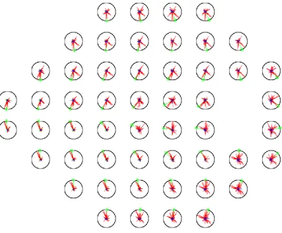
Figure 5. A topographical map describing the relationship between the retinal nerve fibre layer thickness (RNFLT) profile and individual VF points as described by Bayesian Radial Basis Function model II using the 16512 pixel retardation values from the GDxVCC scanning laser polarimetry image. The composition of the graph is the same as Figure 3 and 4 with the green bar with an asterisk indicates the location of expected strongest correlation on the basis of the anatomically derived map from Garway-Heath et al.33 _{In this instance the 'correlation} values' are derived from scaled values in equation (13) and are summarized into 64 sectors for the purpose of comparison.