Rochester Institute of Technology
RIT Scholar Works
Theses Thesis/Dissertation Collections
2010
Threshold interval indexing techniques for
complicated uncertain data
Andrew Knight
Follow this and additional works at:http://scholarworks.rit.edu/theses
This Thesis is brought to you for free and open access by the Thesis/Dissertation Collections at RIT Scholar Works. It has been accepted for inclusion in Theses by an authorized administrator of RIT Scholar Works. For more information, please [email protected].
Recommended Citation
Threshold Interval Indexing Techniques
for Complicated Uncertain Data
Andrew Knight
Computer Science
B. Thomas Golisano College of Computing and Information Sciences
August 31, 2010
Andrew Knight, student
Mangeet Rege, chair
Qi Yu, reader
Abstract
Uncertain data is an increasingly prevalent topic in database research, given the advance of
in-struments which inherently generate uncertainty in their data. In particular, the problem of indexing
uncertain data for range queries has received considerable attention. To efficiently process range queries,
existing approaches mainly focus on reducing the number of disk I/Os. However, due to the inherent
complexity of uncertain data, processing a range query may incur high computational cost in addition
to the I/O cost. In this paper, I present a novel indexing strategy focusing on one-dimensional uncertain
continuous data, called threshold interval indexing. Threshold interval indexing is able to balance I/O
cost and computational cost to achieve an optimal overall query performance. A key ingredient of the
proposed indexing structure is a dynamic interval tree. The dynamic interval tree is much more resistant
to skew than R-trees, which are widely used in other indexing structures. This interval tree optimizes
pruning by storingx-bounds, or pre-calculated probability boundaries, at each node. In addition to the
basic threshold interval index, I present two variants, called thestrong threshold interval indexand the
hyper threshold interval index, which leverage x-bounds not only for pruning but also for accepting
results. Furthermore, I present a more efficientmemory-loadedversions of these indexes, which reduce
the storage size so the primary interval tree can be loaded into memory. Each index description includes
methods for querying, parallelizing, updating, bulk loading, and externalizing. I perform an extensive
set of experiments to demonstrate the effectiveness and efficiency of the proposed indexing strategies.
I. INTRODUCTION
The term uncertain data defines data collected with an inherent and distinctly quantifiable level of uncertainty [2]. Whereas values forcertain data are given as exact constants, values for uncertain data are instead given by probability measures, most notably by probability distribution
functions (PDFs). Uncertain data can be generated from many circumstances:
• Scientific measurements include margins of error due to limited instruments [2].
• Sensor networks are imprecise due to hardware limits [2].
• GPS is only accurate to within a few meters [12].
• Uncertainty in mobile object tracking can magnify errors in predictive queries [2], [52].
• Forecasting weather or economic data is based heavily upon statistics and probabilities [3],
[38], [47].
• Aggregated demographic data only represent summaries, not actual data [4].
• Lost information creates incompleteness in data [38].
Uncertain data is different from erroneous data in that uncertain data, though perhaps not
precise, encapsulates a margin of error or uncertainty as part of its data model, whereas erroneous
data is reported as-is and is assumed to be correct. Just as for certain data, uncertain data values
may be continuous or categorical (discrete), based on the domain of possible values.
The problem of indexing uncertain continuous data for efficiently processing range queries
has received considerable attention in the database community. A set of key strategies have
been proposed and the most representative ones include threshold index [11], [40], the U-tree
[47], and 2D mapping techniques [1], [11]. Most of these approaches assume that disk I/Os
are the dominating factor that determines the overall query performance. Thus, the indexing
structures are usually designed to optimize the number of disk I/Os. However, uncertain data
is inherently more complicated than certain data. Computing a range query on uncertain data
usually involves complicated computations, which incur high CPU cost. This makes disk I/Os no
longer the solely dominating factor that determines the overall query performance. Therefore,
new indexing strategies need to be developed to optimize the overall performance of range
queries on uncertain data.
Uncertain continuous data is usually modeled by PDFs. Some PDFs, like the uniform PDF,
may be very simple to calculate. However, many widely used PDFs involves complicated
computations. For example, computer simulations of cell signaling dynamics for biology research
generate probability distributions with multiple peaks [31]. An example of such functions is
given in Figure 1. Multimodal probability models have also been adopted in many real-world
applications, such as cluster analysis [51].
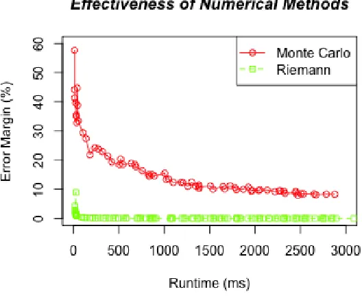
Computing a PDF, such as multimodal probability, may involve high computational cost.
Numerical approaches, such as Monte Carlo integration, have been exploited to improve the
performance. Monte Carlo integration offers a practical technique for multidimensional integrals
because regions can be difficult to define. Tao et al. proposed to use Monte Carlo integration
for efficiently calculating probabilities given arbitrary PDFs [47]. First, the desired region to
integrate is identified. A larger finite region, whose integral is much easier to calculate, is then
defined around the desired region.N points are selected at random within the larger region. The
integral is estimated by the fraction of points within the desired region times the integral of the
Fig. 1: A mixture of four Gaussian distributions, similar to ones in [31]. The four constituent
distributions, shown by the dotted lines, are (µ = 2, σ = 1
3),(µ = 4, σ = 1),(µ = 5, σ =
1),and (µ= 7, σ = 34).
Riemann sum, on the other hand, provides a better strategy for one-dimensional cases. Riemann
sums numerically approximate integrals by calculating the combined area of N rectangles under
a function’s curve [46]. Larger numbers of rectangles mean a smaller error margin. As shown
in Figure 2, Riemann sums are both faster and more accurate than Monte Carlo integrations
for one-dimensional functions. It is also worth to note accuracy is very important for indexing uncertain data. If probabilities are not calculated accurately, then range queries may include invalid objects or exclude valid objects. Indeed, using Riemann sums is very similar to the
argument presented by Agarwal et al. for using histograms with 2D mapping techniques [1]:
histograms, as a series of rectangles, can represent any function to arbitrary accuracy and are
more practical for collecting data.
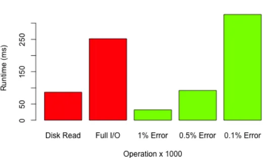
Even though Riemann sums are faster than Monte Carlo integrations in one-dimensional cases,
they still incur high computational cost. As shown in Figure 3, their runtime is significant when
compared to disk I/Os. For high accuracy, probability calculations take even longer than disk
I/Os. Therefore, the number of probability calculations must also be considered if the distribution
Fig. 2: Comparison between Riemann sums and Monte Carlo integration for 1000 random
probability calculations on the multimodal distribution given in Figure 1.
disk I/Os and the CPU cost to achieve an optimal overall query performance.
In this paper, I present a new strategy for indexing one-dimensional uncertain continuous data
called threshold interval indexing. It addresses the weaknesses of previous indexing structures, particularly for handling complicated PDFs, by treating uncertain objects as intervals and thereby
leveraging interval tree techniques. I borrow optimized interval techniques from [7], [8] to build
a dynamic primary tree and store objects in nodes at different levels depending on the objects’
sizes. The notion of using an interval tree to index uncertain data was suggested by Cheng et
al. in [11] but disregarded in favor of an R-tree with extra probability limits called x-bounds. I
assert that x-bounds can just as easily be applied to interval trees to index uncertain data with
special benefits.
The following list summarizes my contributions:
• I presentthreshold interval indexing, a new indexing approach for complicated one-dimensional
uncertain continuous data.
Fig. 3: Runtime comparison between disk I/Os and Riemann sums on the distribution from
Figure 1. A disk read is the time taken to physically read one block of data (4096 bytes) from
the disk. The full I/O is the time to both read and parse the data. The right three bars represent
Riemann sums with different error margins.
– The threshold interval index (TII), which applies x-bounds to nodes.
– The strong threshold interval index (STII), which applies x-bounds to each object.
– The hyper threshold interval index (HTII), which stores x-bounds as intervals.
• I provide efficient methods for querying, building, and maintaining the structures. • I present a memory-loaded strategy to reduce storage size of each structure.
• Iexperimentally prove the success of my indexing strategiesby comparing their performance
results to results from existing strategies.
• I identify appropriate scenarios in which to use different threshold interval indexes based
on experimental performance results.
The different indexes address unique optimizations. The TII presents a universal structure for
threshold interval indexing techniques. The strong TII allows for fewer probability calculations
by storing x-bounds for each object, meaning faster runtime. However, it requires more storage
space. The hyper TII eliminates all probability calculations, but it puts stricter preconditions on
query parameters. The memory-loaded TII loads the entire primary tree into memory because
for updates.
The rest of the paper is organized as follows. Section II explains the motivation for developing
new indexing strategies for complicated uncertain data. Section III presents the basic threshold
interval index. Section IV presents the strong TII based on the design of the TII. Section V
presents the hyper TII, a specialized TII which does not perform any probability calculation
during a query. Section VI describes the memory-loaded strategy threshold interval indexing.
Section VII gives a thorough analysis of performance test results for range queries. Section VIII
discusses related work with uncertain data. Section IX concludes the paper and offers direction
for future research.
II. MOTIVATION FROMPREVIOUS INDEXES
Existing indexes are inadequate for handling complicated uncertain continuous data. This
section will first explain the common data model for handling uncertainty before explaining the
shortcomings of existing structures. The model is known as the uncertain object model or the
probabilistic uncertainty model [1], [11], [12], [38], [44].
A. Data Model
Definition 1: An uncertain attribute e is an attribute whose value is determined by a proba-bility distribution function.
Definition 2: Anuncertain object uis an object containing an uncertain attribute. Denote this attribute as u.e. If u has only one uncertain attribute, then it can be called one-dimensional. If
u.e is a continuous variable, then u can be called continuous.
Definition 3: Theuncertainty domainforuis the domain foru.e’s PDF. Ifuis one-dimensional,
then the uncertainty domain can be called an uncertainty interval. Although theoretically an
uncertainty domain can be infinite, it should be made finite for practicality.
Definition 4: In the uncertain object model, a database table T may hold uncertain objects. Each object is stored in standard relational database tables. Table columns must be homogeneous:
all attribute values in a column must be certain or uncertain.
Indexing continuous uncertain objects improves efficiency of range queries [1], also called
For certain data, an object is either within the query interval or not. For uncertain data, each
object has a probability of being within the query interval, based on its uncertainty domain.
Definition 5: Given a database tableT, aquery interval[a, b]for an attributee, and athreshold probabilityτ, arange queryreturns all uncertain objectsuifromT for whichP r(ui.e∈[a, b])≥
τ.
The range query definition above forms the problem statement. With no index, a query must
calculate a probability for each object to determine if the object falls within the query interval.
Naturally, an efficient index prunes many uncertain objects from a search to avoid unnecessary
probability calculations, which, given the complexity of the PDFs, could save a lot of time.
B. External Interval Tree Index
Interval trees [13] are not specifically designed for handling uncertain data, but one-dimensional
uncertain objects may be treated as intervals by using their PDF endpoints. Arge et al. [7]
propose two optimal external interval tree indexes. Both indexes use a primary tree for layout
and secondary structures to store the objects at each node. The first index’s primary tree is a
balanced tree over a set of fixed endpoints with a branching factor of√B as the base tree, where
B is the block size. The second index replaces the static interval tree with aweight-balanced B-tree[7] storing interval endpoints to achieve dynamic interval management. Note that its primary tree does not store the intervals, it only stores endpoints to control tree spread. In both indexes, each internal node v represents an interval Iv containing all of its child nodes’ endpoints. Each
interval Iv is divided into subintervals called slabs by the endpoint boundaries on v’s immediate child nodes. When using this tree to index a set of interval objects I, an intervali∈I is stored
at the lowest node v in the tree such that i is not split across slab boundaries. Each node v
stores these intervals in secondary structures for each slab boundary: B-trees normally or in an
underflow structure if the number of segments is less than B/2 [7], [23]. These lists hold all intervals that cross the boundary on the left side, on the right side, and as a multislab. Stabbing queries are used to return results.
Since the endpoints in the first index are fixed, it can become unbalanced and therefore
inefficient due to spread and skew in the input interval set. The second index, although much
more complicated, adapts well to skew and to new inputs. However, the downfall of both interval
interval’s endpoints, then few objects are pruned from the search, and a lot of time is wasted in
calculating probabilities. Furthermore, although this external index is theoretically optimal, it is
not always practical [35].
C. Probability Threshold Index
The probability threshold index(PTI) [11] allows range queries to prune more branches from searching than interval indexes allow. The PTI uses a one-dimensional R-tree as a base tree. Only
leaves store uncertain objects. Each internal node has aminimum bounding rectangle(MBR) that encloses the narrowest boundaries [L, R] for all child PDFs. Tighter bounds, called x-bounds, are also calculated for each node. X-bounds are the pair of boundaries (Lx, Rx) such that the probability an object attribute’s value exists in [L, Lx] or [Rx, R] is equal to x [11]. Thus, when performing a range query for objects in [a, b] with probability threshold τ, if, for a certain node,
τ ≥xand[a, b]does not overlap Lx orRx at its right or left ends, then the node and its children may be pruned from the search.
The PTI has many advantages. It is an elegant solution, and it is fairly easy to implement.
The tree is dynamic as well. All boundaries are calculated when objects are added. Multiple
x-bounds can be stored in each node, so queries can choose the most appropriate bounds for its
threshold. Required storage space for internal nodes is relatively small. Note that the U-tree is
very much like a multi-dimensional PTI with additional pruning techniques [47].
The PTI is not without weaknesses, however. The primary weakness pointed out by Cheng et
al. is that differences in interval sizes will skew the balance of the tree [11]. Methods involving
variance-based clustering are provided in [11] to solve this problem; however, they only work
for PDFs that are variance monotonic. Furthermore, Cheng et al. do not provide an optimal
rectangle layout strategy for the PTI’s base tree, the R-tree. The best strategy for any R-tree
is to make MBRs as disjoint as possible. When MBRs overlap too much, extra disk I/Os and
probability calculations must be performed because fewer nodes can be pruned. Adding new
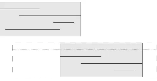
objects, especially objects of vastly different interval lengths, exacerbate overlap, as shown in
Figure 4. Simply put, sloppy R-trees are inefficient, but optimal R-trees are very difficult to
maintain. Strategies such as segment indexes and the SR-tree [25] address different interval
lengths, and interval indexes handle skew very well.
Fig. 4: MBRs can easily become skewed. The dotted rectangle shows how the bottom MBR
must expand to accommodate the uncertain object denoted by the dotted line. These two MBRs
now severely overlap.
be immediately accepted. Since MBRs might overlap, every node must be checked. There is no
exclusivity between node intervals. Nodes may not be stored in any order if their intervals are
stretched. Objects might appear in the overlapping portions of nodes, too. These compounding
factors force probability calculations on all objects in each unpruned node. This wastes lots of
time, especially when the query interval is much larger in size than most uncertainty intervals.
D. 2D Mapping Indexes
Cheng et al. first suggested 2D mapping techniques as an alternative to the PTI for uniform
PDFs [11]. Agarwal et al. then expanded 2D mapping techniques to histogram PDFs [1].
Histogram PDFs can easily be transformed into linear piecewise cumulative distribution functions
(CDFs). A CDFF can then be transformed into a linear piecewise threshold functiong, for which
g(x) gives the minimum value y such that F(y)−F(x)≥ τ for a preset probability threshold
τ. Threshold functions are calculated for each uncertain object and turned into a set of line
segments. A range query for an interval [a, b] graphs the point (a, b) and returns all objects whose line segment threshold functions are below it.
The structures of the indexes presented in [1] manipulate the line segments. The half-plane
range reporting technique partitions the line segments into sets of layers. Queries visit each layer
segment tree, interval tree, and hybrid tree use the same notions presented in [7] about interval
management and slabs to form optimized index structures.
2D mapping indexes are efficient for uniform and histogram PDFs, but they are inapplicable
for more general PDFs. Furthermore, each index is rigidly based upon one threshold value;
separate indexes must be constructed for additional thresholds. This is starkly different from the
PTI, which can manage several threshold values in one structure. However, the application of
interval tree techniques presented in [1] is a novel enhancement over techniques presented in
[7].
III. THRESHOLDINTERVALINDEX
The threshold interval index (TII) addresses the shortcomings of the indexes described in Section II. It is like a dynamic external interval tree, but with x-bounds borrowed from the PTI.
This structure presents two key advantages. The first advantage is that the structure intrinsically
and dynamically maintains balance all the time. The second advantage is that the interval-based
structure makes all uncertain objects which fall entirely within the query interval easy to find and,
therefore, possible to add to the results set without further calculation. The PTI does not allow
this because its MBRs might overlap. Furthermore, adding x-bound avoids the interval index’s
problem for when many uncertainty intervals overlap the query interval. These advantages allow
the TII to handle complicated uncertain data more aptly.
A. Structure
The TII has a primary tree to manage interval endpoints. It also has secondary structures at
internal nodes of the primary tree to store objects. When an object is added to the index, the
endpoints of its uncertainty interval are added to the primary tree. Then, the object itself is added
to the secondary structures of the appropriate tree node. Each object is also assigned a unique
id if it does not already have one. X-bounds are stored for each internal node.
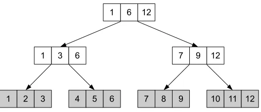
1) Primary Tree: The primary tree is a weight-balanced B-tree with branching parameter
r > 4 and leaf parameter k > 0. The weight of a node is the number of items (in this case, endpoints) below it. All leaves are on level 0. All endpoints are stored at the leaves, and internal
nodes hold copied values of endpoints. The weight-balanced B-tree must hold the following
1 2 3 4 5 6 7 8 9 10 11 12
1 3 6 7 9 12
[image:13.612.176.440.82.195.2]1 6 12
Fig. 5: A weight-balanced B-tree where r = 2 and k = 3. Leaves, shown in gray, store all
uncertain object endpoints. The left and right end values at each node denote the node’s interval.
Parent nodes span their children’s intervals. Node intervals never overlap.
• All leaves have the same depth and weight between k and 2k−1.
• An internal node on level l has weight less than 2rlk.
• An internal node on level l except for the root has weight greater than 1
2r
lk.
• The root has more than one child.
These specifications guarantee that each internal node in the tree has a minimum of(12rlk)/(2rl−1k) =
1
4rchild nodes and a maximum of(2r
lk)/(1 2r
l−1k) = 4rchild nodes [7]. The height of the tree is
O(logr(N/k))[7]. Adjustingr andk control the fan-out of the tree and, consequently, influence the size of the secondary structures stored at each internal node. Thus, the weight-balanced
B-tree provides an effective way to dynamically manage intervals and spread. Figure 5 illustrates
a weight-balanced B-tree.
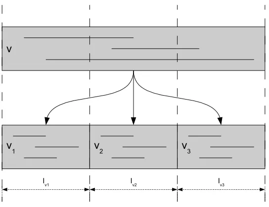
2) Secondary Structures: Each internal node v represents an interval Iv, which spans all interval endpoints represented by children of v. Thus, the c children of v (for 14r ≤ c ≤ 4r) naturally partitionIv into subintervals calledslabs[7]. Each slab is denoted byIvi (for1≤i≤c),
and a contiguous region of slabs, such asIv2Iv3Iv4, is called amultislab [7]. All slab boundaries within Iv are stored in v. Note that Ivi is the interval for the child node vi and that child nodes
are ordered.
An uncertain object is stored atv if its uncertainty interval falls entirely withinIv but overlaps
one or more boundaries of any child node’s Ivi. (A leaf stores uncertain objects whose PDF
v
v1 v2 v3
[image:14.612.171.443.78.288.2]Iv1 Iv2 Iv3
Fig. 6: A node v with three child nodes. The dotted lines denote slab boundaries. Note how
objects are only stored within intervals which can completely contain them.
at exactly one node in the tree, as shown in Figure 6. Let Uv denote the set of uncertain
objects stored in v. In the external dynamic interval index, these objects are stored in secondary
structures called slab lists [7], partitioned by the slab boundaries. However, only two secondary structures are needed per node for the TII because range queries (described later in this section)
work slightly differently than stabbing queries. The left endpoint list stores all uncertain objects in increasing order of their uncertainty intervals’ left endpoints. The right endpoint list stores all uncertain objects in increasing order of their uncertainty intervals’ right endpoints. This is
drastically simpler than the optimal external interval tree, which requires a secondary structure for
each multislab [7]. If the uncertain objects hold extra data or large PDFs, it might be advantageous
to store only uncertainty interval boundary points and object references in the two lists. The actual
objects can be stored in a third structure to avoid duplication.
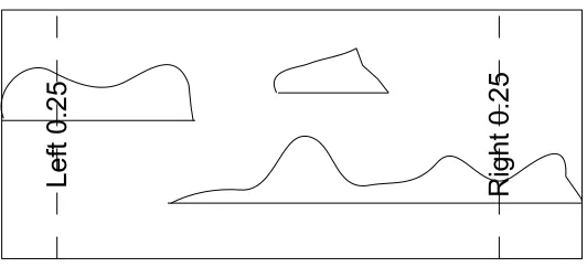
3) Applying X-bounds: X-bounds were introduced as part of the probability threshold index [11] and can easily be applied to the TII.
Le
ft
0.
25
R
ig
ht
0
.2
[image:15.612.174.440.80.201.2]5
Fig. 7: X-bounds are calculated for each node based on uncertain objects’ PDFs. The left and
right 0.25-bounds are tighter than the MBR.
such that
x=
Lx Z
L
f(x)dx=
R Z
Rx
f(x)dx (1)
Lx is the left x-bound, and Rx is the right x-bound. Note that x is a threshold probability
value, meaning 0 ≤ x ≤ 1. For example, if x = 0.25, then there is a 25% chance that the
object’s value appears in the interval [L, L0.25]. Furthermore, there would be a 25% chance it
appears in [R0.25, R] and a 50% chance it appears in [L0.25, R0.25].
The notion of x-bounds can be applied to tree nodes as well as to PDFs, as seen in Figure 7.
The left x-bound for a node is the minimum left x-bound of all child nodes and objects, and
the right x-bound is the maximum right x-bound of all child nodes and objects. Specifically,
for a node v, left and right x-bounds are calculated for Iv. A child node’s x-bounds must be
considered when calculating v’s x-bounds: a child node might have tighter x-bounds than any
of the uncertain objects stored at v. The intervalIv accounts for all uncertain objects stored at v
and in any child nodes of v, and so should the x-bounds. The x-bounds for v’s slabs are given
by the x-bounds on v’s child nodes. All of v’s x-bounds are stored in v’s parent. In this way,
the interval Iv is analogous to a minimum bounding rectangle in an R-tree, and intervals are
tightened by x-bounds in the same way as MBRs are tightened in the PTI [11]. X-bounds for
B. Range Query Evaluation
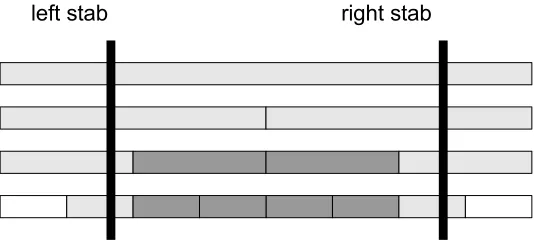
Evaluating range queries for objects in [a, b] with a threshold τ on the TII is like evaluating stabbing queries on a regular interval tree. Twostabsare executed for each endpoint of the query interval: a left stab and a right stab. The nature of the query forces these stabs to be performed
slightly differently from how they are described in [7]. Once the stabs are made, a series of
grabs can be performed for all objects in between. This is called the stab ’n grab search.
1) The Left Stab: The left stab is the most complicated part of the stab ’n grab search. The search starts at the root node and continues down one path through child nodes until it hits
the leaf containing the closest x-bound to a within its boundaries. This leaf is called the left boundary leaf. X-bounds are used to prune this search. Objects are checked at nodes along the stab to see if they belong to the result set.
Theorem 1: Let v be an internal node with child nodes vi for 1≤i≤c. For each child node, let[vi.L, vi.R] be the interval, and let(vi.Lx, vi.Rx)be the left and right x-bounds. Furthermore, let Qbe a range query executed with a query interval [a, b] and a threshold τ ≥x. If vi.Rx < a or vi.Lx> b, thenvi and its children can be pruned from the search.
Proof: The maximum probability that any object stored in vi has a value in [vi.Rx, vi.R] is
x, by the definition of an x-bound. If vi.Rx < a, then the probability that any object stored invi
falls in the query interval must be less than x. Since x ≤τ, there is no way any object stored
in vi could meet the threshold probability. The same argument could be applied for the interval
[vi.L, vi.Lx] when vi.Lx > b.
The appropriate child to choose for each step from parent to child has the minimumifor which
vi cannot be pruned from the search, as shown in Figure 8. Simply put, the leftmost unpruned
child is picked. Remember, child nodes are ordered and do not overlap. A data structure holds
references to all visited nodes so that nodes revisited during the right stab are not reevaluated.
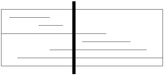
Before moving to the next child node, the uncertain objects stored in secondary structures at
the current node must be investigated, because their uncertainty intervals may overlap the query
interval. If they overlap the query interval, then they might be valid query results. The method
for finding valid results relies on two theorems.
Fig. 8: A left stab is denoted by the thick black line. The stab visits the light gray nodes. The
white nodes are not visited. The dark gray node is pruned based on x-bounds.
Proof: Ifu.R ≤a, then uis completely to the left of the query interval. If u.L≥b, then u
is completely to the right of the query interval. Either way, there is no overlap with the query
interval and therefore a 0% chance of being within it.
Theorem 3: LetQbe a range query with query interval [a, b], and letube an uncertain object with uncertainty interval [u.L, u.R]. If a≤u.L and u.R≤b, then u is a valid query result.
Proof: Since the uncertainty interval for u falls completely within the query interval, there is no chance that u could appear anywhere outside the query interval.
Between the secondary structures, only the right endpoint list is needed. The search on this
list begins by finding the first object whose right endpoint is greater than a. Remember, this list
is sorted, so a binary search can be performed. Any object whose right endpoint is less than a
can be disregarded because of Theorem 2. Each object whose right endpoint is greater than a
must be investigated. Any object whose endpoints are within the query interval is added to the
result set because of Theorem 3. Otherwise, a probability calculation must be performed using
the object’s PDF to determine if it meets the threshold probability. This is shown in Figure 9.
The same strategy applies for the left boundary leaf. All valid objects are added to the result
set.
It is interesting to note that the left stab may visit nodes whose intervals do not contain a.
There could be a situation where a ∈ Ivi yet vi is pruned. In that case, the path of the stab
goes to the next leftmost interval after vi which cannot be pruned, anda will be less than every
uncertainty interval in the new node. (Remember, intervals represented by tree nodes of the same
Fig. 9: Selecting objects from one node during a left stab. All objects to the left of the thick
line can be disregarded. All objects intersecting the thick line require a probability calculation.
in the stab will always be the first element.
2) The Right Stab: The right stab is analogous to the left stab, except it searches with b
instead of a. The leaf found at the bottom of the stab is called the right boundary leaf. X-bound pruning is performed for the rightmost child nodes, not the leftmost. The process for searching
the secondary structures is the same as in the left stab, except “left” and “right” are switched
wherever mentioned. Furthermore, nodes visited during the left stab can be skipped during the
right stab, because the process for investigating uncertain objects accounts for both endpoints of
the uncertainty interval. This is why references to visited nodes are stored during the left stab.
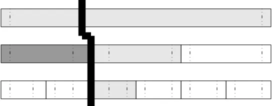
3) The Grabs: The two stabs find the two boundary leaves and some uncertain objects in the result set. The remaining objects to investigate reside in the nodes between the two boundary
leaves. Thankfully, all objects in between can be added to the result set without any probability
calculations.
Theorem 4: Let Qbe a range query with query interval[a, b]. LetvL andvR be the boundary leaves returned by the left and right stabs. Let N be the set of nodes visited by the left and
right stabs. Let S be the set of all nodes v such that v is between vL and vR and v /∈ N. All
uncertain objects stored at all nodes in S are valid query results.
Proof: Every node in the tree between the two boundary leaves, by definition, has an interval that overlaps[a, b]. There are two classes for these nodes: those which overlap the query interval’s endpoints, and those which fall entirely within the query interval. The nodes in N
left stab right stab
Fig. 10: A stab ’n grab query. The light gray nodes are visited during the stabs, and the dark
gray nodes are visited during the grabs. Note how grabbed nodes fall completely within the
query interval.
by the stabs, so they can be ignored outright. All other nodes (internal nodes as well as leaves)
between the boundary leaves therefore fall within [a, b]. Remember, nodes at the same level in
the tree have non-overlapping intervals. The nodes in S are either leaves which directly fall
between the boundary leaves or internal nodes which fall between nodes of the same level in
N. By Theorem 3, the uncertain objects stored at all nodes in S must be in the query interval.
The most effective way to grab all of these uncertain objects is to perform a post-order tree
traversal starting at the left boundary leaf and ending at the right boundary leaf, skipping each
node that has already been visited. No extra searching must be done on the secondary structures.
Figure 10 illustrates a full stab ’n grab query.
4) Time Bounds: A range query can be answered within the following time bounds using the stab ’n grab search:
Theorem 5: LetI be a TII storingN uncertain objects, whose primary tree has branching pa-rameterrand leaf parameterk. Assume any calculation on an uncertain object’s PDF takesO(d)
time. A range queryQwith query interval[a, b]and thresholdτ can return allT uncertain objects stored inI which fall within the query interval with probabilityp≥τ inO(kdlogr(N/k)+T /k)
time.
Proof: The height of the primary tree is O(logr(N/k)) [7]. If the number of child nodes of any internal node is O(r), then the total number of nodes in the tree is O(Σlogr(N/k)
O(rlogr(N/k)) = O(N/k). Since the N uncertain objects are distributed relatively uniformly
over the tree, each node stores O(N/(N/k)) =O(k) objects. A stab, either right or left, visits
O(logr(N/k))nodes from root to boundary leaf and must visit all objects stored at a node in the worst case, calculating probabilities for each. Hence, the stabs are performed inO(kdlogr(N/k))
time. The grabs are performed in O(T /k)time, because extra checking at each node in between the leaf boundaries is unnecessary. All nodes visited by the grabs are guaranteed to be valid
results, so T is used instead of N for the time bound. Therefore, two stabs and all grabs can be
performed in a combined time of O(kdlogr(N/k) +T /k).
5) Parallelization: Range queries on the TII can easily be parallelized because each object is stored at exactly one node and branches eventually diverge from each other. Define thediverging node as the first node in the tree for which the left and right stabs proceed to different children. In the worst case, the diverging node is the root; in the best case, there is no diverging node,
meaning the left and right boundary leaves are the same leaf. The left and right stabs can start
at the same time as one stab. After the diverging node is reached, the left and right stabs can be
executed on separate threads, because they traverse nodes from that point forward. Furthermore,
each branch in between the left and right stabs must be “grabbed,” so another thread can be
spawned for each branch. Each thread only visits nodes going from top to bottom.
C. Maintenance
When performing updates to the TII, both the primary tree and the secondary structures must
be changed.
1) Insertion: When an uncertain object is inserted, both of its uncertainty interval endpoints are first added to the primary tree. The process for maintaining a weight-balanced B-tree is fully
described in [8]. Let r be the branching parameter and k be the leaf parameter. An element is
added to the appropriate leaf v. If v now has 2k elements, it is split across a boundary b into two leaves v and v0 holding k elements each, and a reference to v0 is stored in the parent node.
Each time a split occurs, the parent may exceed its weight limit of 2rlk, so splits are cascaded up the tree as necessary. Splits for parent nodes may not always create equal halves, but the
weight restrictions can always be met.
When a node v is split across a boundary b, its two endpoint lists must also be split. The
the boundary (right endpoint ≤ b), (2) objects which are entirely to the right of the boundary
(left endpoint ≥ b), and (3) objects which intersect the boundary (left endpoint ≤ b ≤ right
endpoint). Objects in the first set remain at v. Objects in the second set are moved to the new
node v0. Objects in the third set must be moved to the parent node. Since the lists are sorted,
binary searches and hash tables can optimize the partition. This process is much easier than the
process described in [8] because the TII only uses two lists per internal node.
Once the uncertain object’s endpoints are inserted into the primary tree and all nodes are split,
the object itself is inserted into the left and right endpoint lists of the appropriate node. A binary
search on each list can optimize these insertions.
Finally, the x-bounds (u.Lx, u.Rx) are calculated for the object. Let (v.Lx, v.Rx) be the x-bounds for the node v into which the object is being stored. Ifu.Rx > v.Rx, thenu.Rx becomes
the new right x-bound forv. Likewise, if u.Lx< v.Lx, thenu.Lx becomes the new left x-bound
for v. The new object’s x-bounds “tighten” the node’s x-bounds in these two cases. Changes in
x-bounds should cascade up to parent nodes as necessary.
Theorem 6: Let I be a TII storing N uncertain objects, whose primary tree has branching
parameter r and leaf parameter k. Assume any calculation on an uncertain object’s PDF takes
O(d) time. An uncertain object can be added to I with an average time of O(logr(N/k) +
log2k+d) =O(logN +d) and a worst-case time of O(kdlog2klogr(N/k) +d).
Proof: For the average case, a leaf will not need to be split. Finding the leaf into which to insert the object takes O(logr(N/k)) (the height of the tree), and inserting the object into the secondary structures takes O(log2k). Adjusting slab boundaries and x-bounds takes O(d). Therefore, the average insertion time is O(logr(N/k)) +O(log2k) +O(d) = O(log(N/k) +
logk +d) = O(logN +d). For the worst case, nodes must be split. Since each node stores
O(k) objects, partitioning the list of objects takes O(k). The parent node’s list must be resorted because of its new elements, which takes O(klog2k). Thus, every split takes O(klog2k). Since parents might need to be split as well, the total number of splits is O(klog2klogr(N/k)). X-bounds must be recalculated for every split node. After inserting the object into the right node
as in the average case, the worst case time becomes O(logr(N/k)) +O(kdlog2klogr(N/k)) +
O(logr(N/k) +log2k+d) = O(kdlog2klogr(N/k) +d).
its endpoints in the primary tree are flagged. Once half of the objects have been deleted from
the index, the whole index is reconstructed.
Changing the x-bounds stored at the node from which the object is deleted is difficult for the
TII because x-bounds are not stored for each uncertain object. When an object is deleted, there
are two alternative strategies for handling x-bound updates. The first strategy is very simple: do
not change the x-bounds. Although the x-bounds will not be as tight as possible, they will still
prune away nodes. No extra work must be done for this strategy. If the index is reconstructed,
then x-bounds will automatically be updated for the new structure. The second strategy would be
to replace the x-bounds if necessary. This means the x-bounds for every uncertain object stored
at the node must be calculated and the tightest left and right from this set must be identified. If
these new x-bounds are looser than the node’s previous x-bounds, meaning the object removed
had the tightest x-bounds in the node, then the node’s x-bounds are set to these new values.
Then, the x-bounds of all parents of the node must be checked as well. Certainly, the second
strategy involves a lot of extra work. For most implementations of the TII, the first strategy is
recommended.
Theorem 7: Let I be a TII storing N uncertain objects, whose primary tree has branching
parameter r and leaf parameter k. Assume any calculation on an uncertain object’s PDF takes
O(d) time. An uncertain object can be deleted from I in O(logr(N/k) +log2k) = O(logN)
time.
Proof: Finding the object to delete is analogous to the process for insertion proved in Theorem 6, minus the O(d) used to update x-bounds.
Corollary 1: A full deletion involving updated x-bounds can be performed inO(dlogr(N/k)+
kd) time.
Proof: After the object is found and deleted from the secondary structures (which takes
O(logr(N/k) +log2k)), x-bounds for all objects at that node must be calculated, which takes
O(kd) time. Then, x-bounds of all parents must be checked against potentially new x-bounds, which takes O(d) per parent for up to O(logr(N/k)) parents. The total deletion time is then
D. Bulk Loading
Bulk loading the TII can be performed for the primary tree just like bulk loading can be
performed on any B-tree [41]. The trick is to maintain proper weight and balance when building
the primary tree. Remember, for branching parameter r and leaf parameter k, leaf weight must
be between k and 2k−1, and internal node weight for level l must be between 12rlk and 2rlk. Before bulk loading runs, the list of uncertain objects’ uncertainty interval endpoints is sorted.
Each endpoint is handled as an independent value; it is not associated with its other endpoint.
Bulk loading runs in levels, starting at level 0 (the leaves) and ending when there is one node
at the top (the root). At level 0, the list of endpoints is divided into contiguous sublists of2k−1
elements each. If the last list has less than k elements, an element from previous lists can be
forwarded until each list has at least k+ 1 elements. A leaf node structure is created for each sublist, using its minimum and maximum elements as slab boundaries. This leaf should have
two empty lists for its secondary structures as well as fields for its interval boundary [L, R]
and x-bounds (Lx, Rx). Initially, Lx =R and Rx = L because the leaf does not yet hold any uncertain objects. (With these trivial x-bounds, the leaf will always be pruned. As soon as the
first object is added, these x-bounds will be overwritten.)
For each subsequent level l, the list of slab boundaries is used to build internal nodes and
create intervals for children. This list contains the slabs for each leaf in order. Whenever two
adjacent slabs don’t share the same right/left boundary, either boundary may be chosen to preserve
continuous intervals. The list is divided into contiguous sublists ofrelements each. Again, if the
last list has fewer than r elements, elements can be added until it has at least 14r. The sublists are turned into internal nodes, constructed much like the leaves mentioned for level 0. However,
nodes built in the previous level are added as child nodes, in order, to these internal nodes.
Each internal node receives r children. Because there is one slab in the remainder list for each
child node, each parent node has exactly enough pointers for r children, and all children are
guaranteed to have a parent. Ordering is important because the elements from each remainder
list divide the child nodes into slabs. Furthermore, the fan-out of r preserves weight balance.
Theorem 8: When bulk loading a B-tree T, grouping elements by 2k at level 0 and by r at any level l > 0 makes T a weight-balanced B-tree.
weight of each leaf is2k−1. Even if extra elements must be added to the last leaf in the list, each leaf will have at least k elements. This meets the boundary condition for leaves. For an internal
node at level 1, there are r child nodes, meaning the weight is r(2k−1) = 2rk−r < 2r1k. Even if extra elements must be added to the last internal node, there will be at the very least
1
4r + 1 elements per node, and the ratio of children to parents remains one to one. For an
internal node at level l, the weight becomes r(2rl−1k−rl−1) = 2rlk−rl <2rlk. Furthermore,
2rlk−rl = (rl)(2k−1)≥ 1 2r
lk because2k−1≥ 1
2k. (This lower bound also holds for 1 4r+ 1).
Both boundary conditions are met for internal nodes. Bulk loading stops when only one node
is left as the root. All these meet the qualifications for a weight-balanced B-tree.
After the primary tree is constructed, each uncertain object is inserted into the secondary
structures of its appropriate node as described in the bottom part of Section III-C1. Unfortunately,
these objects cannot be efficiently added while bulk loading the tree because every uncertainty
interval would need investigation every time a node is constructed. X-bounds are calculated
from the bottom-up after all objects have been added. Calculating them each time an object is
added results in a massive amount of recalculation, since x-bounds for child nodes may influence
x-bounds for their parents.
Theorem 9: A set of N uncertain objects can be bulk loaded into a TII in O(NlogN+N d)
time.
Proof:Sorting the list of uncertain objects takesO(NlogN)time. For building the primary tree, let T(n) represent the time to build the tree starting at the leaves, and let S(n, i)represent the time to build the levels of nodes for all levels l ≥ i. T(n) = S(n/(2k),1) + Θ(n/(2k))
because the level of leaves has n/(2k) nodes. S(n, i) = S(n/r, i+ 1) + Θ(n) because n/r
new nodes are created at level i, but n children from level i−1 must be attached to the new nodes. According to case 3 of the master method [13], S(n) = Θ(n) and T(n) = Θ(n). Once the primary tree is constructed, inserting an object into its appropriate secondary structure and
E. Externalization
The TII can easily be externalized by settingk and rfor the primary tree appropriately, albeit
differently than how described in [7]. Let B be the block size; specifically, the number of data
units which can be stored in a block. For the primary tree, an uncertain object is represented only
by its uncertainty interval endpoints, each of which is one unit of data. Each child node needs
two units for endpoints, one unit for its block pointer, and two units for each set of x-bounds,
meaning each node requires 3 + 2n units, wherenis the number of x-bounds stored for the tree. The number of children per node still ranges from 14r to 4r. Thus, to fit each primary tree node into one block, k = 12B and r= 4(3+21 n)B. The external weight-balanced B-tree then maintains the following properties:
• All leaves have the same depth and weight between 12B and B−1.
• An internal node on level l has weight less than B( B
4(3+2n))
l.
• An internal node on level l except for the root has weight greater than 1
4B(
B
4(3+2n))
l.
• The root has more than one child.
Each node uses one block to store intervals, x-bounds, and child pointers, and each secondary
structure uses O(1) blocks to store its objects. In [7], k = 12B and r = 14√B to guarantee that each internal node has Θ(√B) children. The reasons and proofs for using these parameters are
explained in [7]. The primary reason for selecting a fan-out of √B for the external interval
tree is to ensure the number of blocks is limited to O(1) for each leaf, each slab list, and each internal node’s pointers. If the uncertain objects stored in the TII are relatively small in size,
then the same upper bounds apply for the number of disk I/Os. However, if the objects are large
in size, which may be the case given how the PDFs are stored, then more blocks will be needed
for secondary structures. Tight space bounds cannot be placed on the secondary blocks. It would
be best to let the DBMS hold default PDF types and store arguments for these PDFs in the
databases to reduce storage size; for example, the index would store three values for type, mean,
and standard deviation for a normal PDF. Nicely, though, the number of blocks needed for the
primary tree does not change, because it only stores interval endpoints. The value ofr given for
the TII is appropriate given the necessity of x-bounds. Naturally, extra metadata might force the
values of k and r to be slightly smaller.
answered using O(logBN +T /B) disk I/Os and O(BlogBN) probability calculations, and updates can be performed using O(logBN) disk I/Os and O(1) probability calculations.
Proof:Substituter= 4(3+21 n)B andk = 12B. The bounds from [7] still remain for disk I/Os. Each node uses O(1) blocks to store bounds and pointers to child nodes, and each endpoint list uses O(1) blocks as well. Since there are O(N/k) nodes, the tree is stored inO(N/B) blocks. For range queries, O(logB(N/B)) =O(logBN) I/Os are used for each stab and O(T /B) I/Os are used for the grabs for a total of O(logBN+T /B) I/Os. Probability calculations must only be performed on stabs, not grabs. The number of calculations for each block is O(k) =O(B), so the total number of calculations is O(BlogBN). Update bounds for disk I/Os follow from the same analysis for stabs, and O(1) probabilities must be calculated for the node into which the object is inserted. Splits do not require more probability calculations.
IV. STRONGTHRESHOLDINTERVAL INDEX
The threshold interval index applies x-bounds to primary tree nodes, which can only be used
to prune nodes from a query during a stab. Uncertain objects can only be accepted as valid
results without extra calculation during the grabs. If an object visited during a stab overlaps the
query interval boundaries, an expensive probability calculation must be performed. The strong
threshold interval index (STII) presented in this section allows uncertain objects to be accepted during stabs without probability calculations by storing x-bounds for each object. These x-bounds
can be stored by making minor changes to the TII.
A. Structure
The structure for the STII is almost identical to the TII. The primary tree is the same. X-bounds
are applied to nodes in the same fashion. Each node stores the objects contained exclusively
within its interval. The difference for the STII is in the secondary structures.
For the STII, all objects for a node are stored in one list sorted by id. This list, called the
object map, should store id, PDF, and any other data associated with the object, but not x-bound values. Then, for each x-bound threshold value, two additional lists are needed. These lists store
the x-bound pair(Lx, Rx)and id for each object in the object map. One list stores x-bound pairs ordered from least to greatest using Lx, and the other list orders x-bound pairs using Rx, much
1 + 2n lists per node, where n is the number of x-bound threshold probabilities for the index.
It is mandatory that x = 0.0 and x = 1.0 (for 0% and 100% respectively) be included among
the x thresholds for the correctness of the range query algorithm.
X-bound pairs are stored in separate lists from the objects because each x-bound list must
be sorted for range queries. Since PDFs are arbitrary, object orderings might be different based
on various x values. For example, a skewed-left distribution and a skewed-right distribution
will have different x-bounds even if they share the same endpoints. The object map maps ids
to objects, so objects can be quickly fetched based on any x threshold probability ordering.
Separating x-bounds from objects also allows for fewer disk I/Os during a query, which will be
explained in later subsections.
B. Range Query Evaluation
Again, range queries over the STII are nearly identical to range queries over the TII. The stab
’n grab search is the same: perform two stabs to find left and right boundary leaves, and grab all
nodes in between. Pruning during the stab is also the same, since it uses the nodes’ x-bounds.
The query can be parallelized by the same method as for the TII, too, since parallelization
relies on paths through the tree. The primary change for the STII is in how the query stabs an
individual node.
A stab can automatically accept many objects as valid results when visiting a node in the
STII. When a stab visits a node, it must fetch the object map. It must also fetch the appropriate
x-bound lists. For a left/right stab, the x-bound list to fetch must be sorted by right/left endpoint,
respectively. This is similar to the left and right endpoint lists for TII nodes. The x values to
use depend on the query threshold τ. Two lists are needed, one for which x ≤ τ, called the
pruning list, and one for which x ≥ τ, called the accepting list. Denote these x values as xp and xa, respectively. When pruning, xp ≤ τ ensures that all objects ignored do not qualify
for the threshold probability. When accepting, xa ≥ τ ensures that all objects accepted have a
probability of at least τ for being a valid result. This is why x = 0.0 and x = 1.0 must be included as threshold probabilities in the index, so that no matter what value τ the query uses,
there will always be an x such that x ≤ τ for pruning and x ≥ τ for accepting. Figure 11
illustrates the difference between pruning and accepting thresholds. If the index stores an x
0.1 0.2 0.3
Fig. 11: Pruning vs. accepting x values. This uncertain object stores x-bounds for x= 0.1 and
x= 0.3, but suppose τ = 0.2. The left-0.1-bound cannot be used to accept this object because the diagonally-shaded region does not cover enough area, and the left-0.3-bound cannot be used
to prune this object because the gray region holds enough area to satisfy τ at unknown points.
Otherwise, two different x-bound lists are needed, and the two values for x should be as close
to τ as possible.
Once the appropriate x-bound lists are fetched, the objects are sorted in order of the pruning
list. The first object whose x-bound falls within the query interval is found using a binary search.
For a left/right stab, this is a right/left x-bound, respectively. This prunes all objects which cannot
fall within the query interval. Every subsequent object in the list is then visited. Theorem 11
provides conditions for accepting objects as valid results:
Theorem 11: Let u be an uncertain object with uncertainty interval [u.L, u.R] and x-bounds
(u.Lx, u.Rx). Let Q be a range query with query interval [a, b] and probability threshold τ. If
x≥τ, and if any one of the following four conditions is true, then u is a valid result for Q:
1) [u.L, u.Lx] is entirely within [a, b] 2) [u.Rx, u.R] is entirely within [a, b]
3) 1−2x≥τ and [u.Lx, u.Rx] is entirely within [a, b] 4) Rabu.P DF(x)dx≥τ
Proof: (1) (2) By definition of x-bounds, Ru.Lx
u.L u.P DF(x)dx= Ru.R
Fig. 12: STII node stab conditions. The two thick vertical bars represent the query interval,
and shaded regions represent x-bound regions. The first object’s left x-bound region is within
the query interval (1), as is the second object’s right x-bound region (2). The third and fourth
objects’ middle regions are entirely within the query interval. Suppose x= 0.3, which is likely for the third object: it can be accepted (3). Suppose however x = 0.45, which is likely for the fourth object: a probability calculation will be required (4). Note that in a real object list, these
objects would be sorted by x-bounds, and objects would not have mixed x values.
τ. Therefore, both regions satisfy τ, and u is a valid result of Q. (3) The area under all of
u.P DF is 1.0. The sum of area under u.P DF for the two intervals mentioned in (1) and (2) is 2x. Therefore, the remaining area for the interval [u.Lx, u.Rx] is 1−2x. If 1−2x≥ τ and
[u.Lx, u.Rx] is entirely within [a, b], then u still qualifies as a result of Q. (If x ≥0.5 and the
x-bound interval is backwards, this condition is voided anyway because 1−2x ≤ 0 ≤ τ.) (4)
Rb
au.P DF(x)dx = Pr(x ∈ [a, b]). This is the problem statement from Section II. Figure 12 illustrates each of the four conditions.
Note that conditions (1), (2), and (3) use x-bounds stored in the accepting list (maintaining
the precondition that xa ≥τ). This means that a probability calculation is not performed unless
condition (4) is needed. This is why both the pruning list and accepting list are needed: the
pruning list for the binary search, and the accepting list for the conditions.
The time bounds for a range query using the STII are the same as for the TII, given in
C. Maintenance, Bulk Loading, and Externalization
Methods for maintenance, bulk loading, and externalization for the STII are nearly identical
to the methods used for the TII. Again, the difference is handling x-bounds for each object.
a) Insertion: When each object is added, its x-bounds for all x values must be calculated. The object is inserted into the object map of the appropriate node, and its x-bounds are inserted
into the other lists. Each list insertion uses a binary search. Since these insertions all have the
same time bounds, their summation is simply a constant factor. Therefore, the time bounds
presented in Theorem 6 for the TII also hold for the STII.
b) Deletion: When an object is deleted, its x-bounds must also be removed from the secondary structures. They could be difficult to find for each x-bound list, so it would be best to
calculate all x-bounds first and then use binary searches to find all values to delete. Theorem 7
can be applied to the STII for time bounds by similar arguments in its proof. Furthermore, a
full deletion would be more feasible, since x-bounds are already calculated for each object.
c) Bulk Loading: The TII’s bulk loading algorithm disregards individual objects’ x-bounds after storing x-bounds for the nodes. The STII’s bulk loading algorithm must store them instead.
The best time to calculate x-bounds for each object is when the object is inserted into the index,
after the primary tree is built. This way, each object and its x-bounds are inserted in order. When
applying x-bounds to tree nodes, all values are already calculated. Again, time bounds are the
same as given in Theorem 9.
d) Externalization: Secondary structures must be formatted differently for effective exter-nalization. Each object map and list of x-bounds should have its own set of blocks. This way,
during a query, only the blocks for the object map and appropriate x-bound lists must be read,
saving time instead of reading all blocks. The bounds for index storage size and number of disk
I/Os for a query remain the same as for a TII, given in Theorem 10.
V. HYPER THRESHOLDINTERVALINDEX
The threshold interval index uses x-bounds to prune branches from a query search. The strong
version uses x-bounds both to prune and to accept results at the object level. For both, however,
probability calculations are always required when results can neither be pruned nor accepted,
x-bounds purely for accepting valid results and never performs any probability calculations.
X-bounds for each object are stored as intervals in an interval tree. This structure is much different
from the TII and STII. While the promise of no probability calculations is desirable, the HTII
is limited in query interval size and can only hold one x-bound threshold probability.
A. Structure
As with other threshold interval indexes, the HTII has a primary tree with secondary structures.
However, the key difference in the HTII is that it does not store uncertain object intervals in its
primary tree. Instead, it stores threshold satisfier intervals.
Definition 7: Letube an uncertain object with an uncertainty interval[u.L, u.R]and x-bounds
(u.Lx, u.Rx). Given a probability threshold value x, a threshold satisfier interval (or threshold
satisfier for short) is an interval [Ls, Rs]within [u.L, u.R]such that RRs
Ls u.P DF(x)dx=x. The
left threshold satisfier is the interval [u.L, u.Lx], and the right threshold satisfier is the interval
[u.Rx, u.R].
A threshold satisfier for an uncertain object satisfiesa query probability threshold. Thus, if a threshold satisfier falls within a query interval, and the probability thresholds are equal, then the
object can be accepted as a valid result without a probability calculation at query time. Indeed, the
intervals built using the accepting list during STII queries are, by definition, threshold satisfiers.
Only two probabilities are calculated for x-bounds each time a new object is added to the index.
Figure 13 depicts an uncertain object with two pairs of threshold satisfiers.
The HTII is built using one threshold probability value x. The HTII’s primary tree stores both
left and right threshold satisfier intervals for each uncertain object using x. This means four
endpoints are inserted into the weight-balanced B-tree for each uncertain object. The secondary
structures hold both threshold satisfiers and uncertain objects. If a tree node v covers an interval
Iv, then all threshold satisfiers which fall entirely within Iv and overlap child node intervals are
stored in the secondary structures for v. For each node, there are three secondary structures. A
left endpoint list stores threshold satisfiers sorted by left endpoint. A right endpoint list stores threshold satisfiers sorted by right endpoint. (The “left” and “right” specifications for these
endpoint lists refer to ordering of satisfiers. It does not divide left and right threshold satisfiers; both left and right satisfiers are stored together in both lists.) Finally, all uncertain objects which
left-0.4-bound right-0.4-bound
[image:32.612.184.420.111.278.2]right-0.6-bound left-0.6-bound
Fig. 13: Threshold satisfiers on an uncertain object for x = 0.4 (top) and x = 0.6 (bottom). Threshold satisfiers overlap when x >0.5.
map. Each threshold satisfier must store the id of its uncertain object so that when threshold satisfiers are accepted during a query, the object to which it refers can quickly be retrieved from
the object map.
Note that an object will be stored in two different nodes if its left and right satisfiers fall into
different nodes. Thus, x-bounds are not stored for primary tree nodes, because x-bounds cannot
be calculated when objects span two nodes. This distinguishes the HTII from the TII and STII
and more closely resembles the dynamic interval index presented in [7]. Also note that only
one probability threshold value can be stored using this index, since threshold satisfiers are the
primary intervals stored, not the uncertain objects themselves.
B. Range Query Evaluation
As with all threshold interval indexes, the HTII uses a stab ’n grab approach for range queries.
Although the conditions for finding results are simpler, queries must meet two preconditions in
order to guarantee validity:
Object 1
Object 2
[image:33.612.175.439.72.307.2]Object 3
Fig. 14: A left stab for an HTII node. Two threshold satisfiers fall entirely within the query
interval, so their objects are valid results. Note how only one of the threshold satisfiers for an
object must be within the query interval to meet the query’s probability threshold.
2) The query’s interval length must be greater than or equal to the largest object interval
length.
The query algorithm must be explained before the preconditions can be fully understood.
1) Stab ’n Grab Alterations: Range queries use a simpler stab ’n grab search than the version used for the TII. Since the HTII nodes do not store x-bounds, there is no x-bound pruning for
branches. The procedure for finding boundary leaves and grabbing nodes in between remains
the same. Again, the difference is in retrieving results from an individual node stab.
Stabbing an individual node is fairly straightforward, shown in Figure 14. The appropriate
list of threshold satisfiers is needed: sorted by left endpoint for a left stab, and sorted by right
endpoint for a right stab. Note how this is different than for the TII, in which any object interval
that overlapped the query interval needed investigation. For the HTII, only threshold satisfiers
which fall completely within the query interval are of interest, because, otherwise, they do not
satisfy the query probability threshold. Thus, a left stab performs a binary search to find the
endpoint (likewise with right endpoints for a right stab). Every subsequent threshold satisfier
from this point forward must meet only one condition: it must fall entirely within the query
interval. The ids for qualifying threshold intervals fetch the valid objects from the object map.
No probability calculations are needed.
Duplicate results are an unfortunate side effect when using the HTII. If both left and right
threshold satisfiers for an object fall within a query interval, an object might be reported twice
by two different nodes. Simple hashing storage techniques or a results scan after performing the
query can eliminate duplicate objects from the result set.
2) Preconditions: The first precondition is that the query’s probability threshold must equal the probability threshold used to build the index. As mentioned earlier, the HTII can only be built
upon one threshold value, in contrast to the TII and STII which can store multiple thresholds.
If the query’s threshold is larger than the index’s threshold, then the threshold satisfiers are
not large enough to give acceptable results. If the query’s threshold is smaller than the index’s
threshold, then some objects can be accepted, but other objects may be overlooked since their
threshold satisfiers would be too large and marked as invalid. Threshold satisfiers must have
equal probability to the query threshold.
The second precondition for the HTII is that query interval length must be at least as large as
the largest object interval length in the index. Theorem 12 provides the basis for this precondition.
Theorem 12: Let Q be a range query with interval [a, b] and probability threshold τ. Let u
be an uncertain object with uncertainty interval [u.L, u.R]. For u to be accepted or rejected as a valid result of Q using only its left and right threshold satisfiers, the smallest value possible
for the query interval length (b−a) must be u’s uncertainty interval length (u.R−u.L).
Proof: The left and right threshold satisfiers for u are [u.L, u.Lτ] and [u.Rτ, u.R], respec-tively. Each covers a probability of exactly τ. Suppose a query interval [a, b] has a length less than the object interval length. Then, there is a chance that the query interval falls entirely within
the object interval. The threshold satisfiers would be of no use, since they would both partially
fall outside of the query interval. The only way to accept or reject u would be to perform a
probability calculation. However, if the query interval length is equal to or greater than the object
interval length, then at least one threshold satisfier must always fall within the query interval if
u is a valid result. If u is valid and a = u.L, then both left and right threshold satisfiers for
![Fig. 1: A mixture of four Gaussian distributions, similar to ones in [31]. The four constituent](https://thumb-us.123doks.com/thumbv2/123dok_us/54407.4992/5.612.164.431.90.285/fig-mixture-gaussian-distributions-similar-ones-constituent.webp)